Article

Hyperspectral Anomaly Detection via Dual Dictionaries Construction Guided by Two-Stage Complementary Decision

1
School of Aerospace Science and Technology, Xidian University, Xi’an 710126, China
2
Shaanxi Academy of Aerospace Technology Application Co., Ltd., Xi’an 710199, China
*
Author to whom correspondence should be addressed.
Remote Sens. 2022, 14(8), 1784; https://doi.org/10.3390/rs14081784
Submission received: 8 March 2022 / Revised: 4 April 2022 / Accepted: 5 April 2022 / Published: 7 April 2022

Abstract

:
Low rank and sparse representation (LRSR) with dual-dictionaries-based methods for detecting anomalies in hyperspectral images (HSIs) are proven to be effective. However, the potential anomaly dictionary is vulnerable to being contaminated by the background pixels in the above methods, and this limits the effect of hyperspectral anomaly detection (HAD). In this paper, a dual dictionaries construction method via two-stage complementary decision (DDC–TSCD) for HAD is proposed. In the first stage, an adaptive inner window–based saliency detection was proposed to yield a coarse binary map, acting as the indicator to select pure background pixels. For the second stage, a background estimation network was designed to generate a fine binary map. Finally, the coarse binary map and fine binary map worked together to construct a pure background dictionary and potential anomaly dictionary in the guidance of the superpixels derived from the first stage. The experiments conducted on public datasets (i.e., HYDICE, Pavia, Los Angeles, San Diego-I, San Diego-II and Texas Coast) demonstrate that DDC–TSCD achieves satisfactory AUC values, which are separately 0.9991, 0.9951, 0.9968, 0.9923, 0.9986 and 0.9969, as compared to four typical methods and three state-of-the-art methods.

Graphical Abstract

1. Introduction

Hyperspectral images (HSIs), which have the characteristics of a wide spectral range and high spectral resolution, are widely utilized to discriminate physical properties of different materials [1]. Benefitting from the rich spectral information, HSIs are active in the field of image classification [2,3], hyperspectral unmixing [4,5], band selection [6,7], anomaly detection [8,9] and target detection [10,11]. Among these applications, hyperspectral anomaly detection (HAD), aiming to excavate the pixels with significant spectral difference relative to surrounding pixels [12], attracts particular interest. Compared with the hyperspectral target detection, the absence of the prior information makes HAD more challenging.
In the past decades, the visual saliency detection theory [13,14], aiming to highlight the most attractive and distinctive regions in a scene, has been widely used in the field of AD [15,16]. Among them, the context-aware saliency detection [17] is commonly adopted to act as the technique to search for salient objects, due to its powerful performance. For the HAD task, the saliency objects in HSI can be reckoned as anomalies, and, hence, the context-aware saliency detection method may be a useful tool to detect anomalies in HSI.
Recently, the autoencoder (AE) has aroused widespread concern in the field of HAD, due to the fact that AE has a strong ability to characterize the background and anomalies compared with the traditional methods. Similarly, the generative adversarial network (GAN) has attracted increasing attention, owing to the strong generalization ability in regard to high-dimensional, unlabeled, and limited samples [18]. With this condition, combining AE and GAN may be helpful to perform excellent background reconstruction and poor anomaly reconstruction.
Additionally, low rank and sparse representation (LRSR) with dual-dictionaries-based methods are proven to be effective to detect anomalies in HSIs. The most typical LRSR with a dual-dictionaries-based method is the PAB-DC method, which was proposed by Huyan et al. [19]; it jointly considers the background dictionary and potential anomaly dictionary to perform LRSR. However, for the PAB-DC method, due to its limited capability to characterize the background and anomalies, the construction of the potential anomaly dictionary is vulnerable to being contaminated by the background pixels, which is harmful to the detection performance. To illustrate this situation, we provide an example to display the construction results of background and potential anomaly dictionaries in PAB-DC, which are separately represented in Figure 1(I-a,I-b).
Considering the above three aspects, we intended to employ the combination of AE and GAN to assist the construction of pure background and potential anomaly dictionaries. However, the presence of the anomalies in the training stage limits the learning effect. To this end, a preliminary purification work should be considered in advance.
Toward this goal, we propose a dual dictionaries construction method via two-stage complementary decision for HAD, as illustrated in Figure 2. Concretely, for the first stage, a coarse background–anomaly separation strategy, which is implemented by the saliency detection based on the adaptive inner window, is proposed to acquire a coarse binary map. In the second stage, a background estimation network (BEN) is designed to yield a fine binary map, in which the training samples for BEN’s learning stage are derived from the guidance of the coarse binary map. Finally, the coarse binary map and fine binary map are jointly to generate the indicators to guide the selection of the atoms for background and potential anomaly dictionaries. Notably, the fact that there is a large number of atoms in the background indicator will result in high computation complexity, and, hence, the superpixels are used to act as a selector of background to further screen the atoms. To verify the superiority of the proposed method, we visualized the construction effect of background and potential anomaly dictionaries of proposed method, as illustrated in Figure 1(II-a,II-b). By observing Figure 1, we can see that there is a slight difference between PAB-DC and the proposed method on background dictionary, while atoms belonging to the potential anomaly dictionary for the proposed method are evidently purer than those of PAB-DC.
The main contributions of this paper are as follows:
(1)
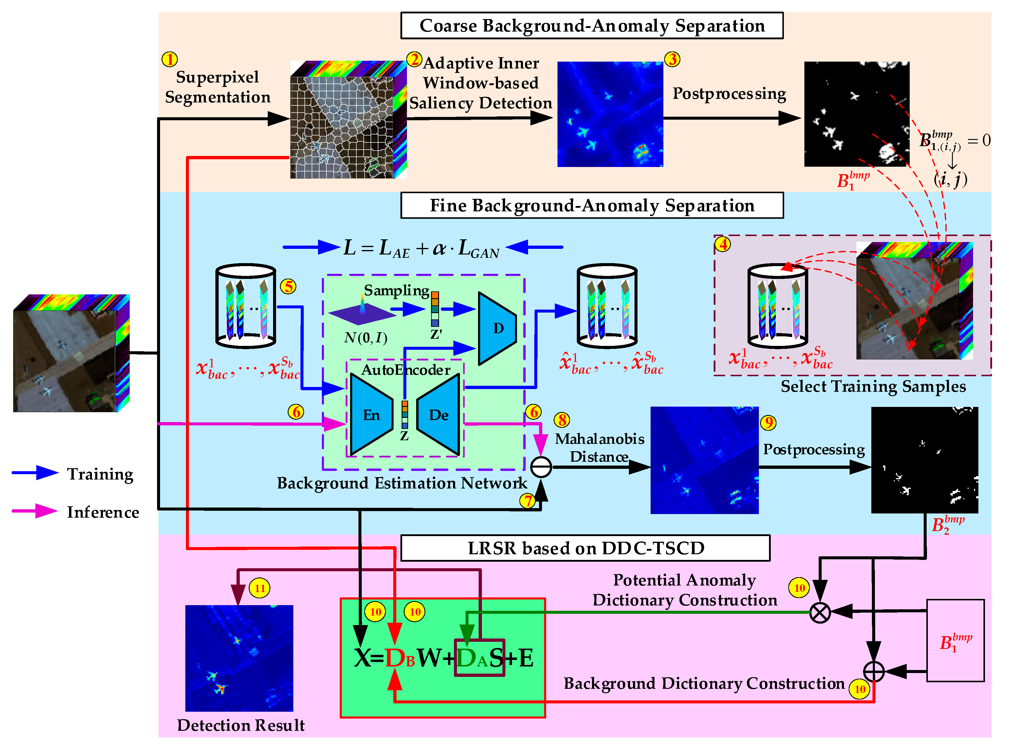
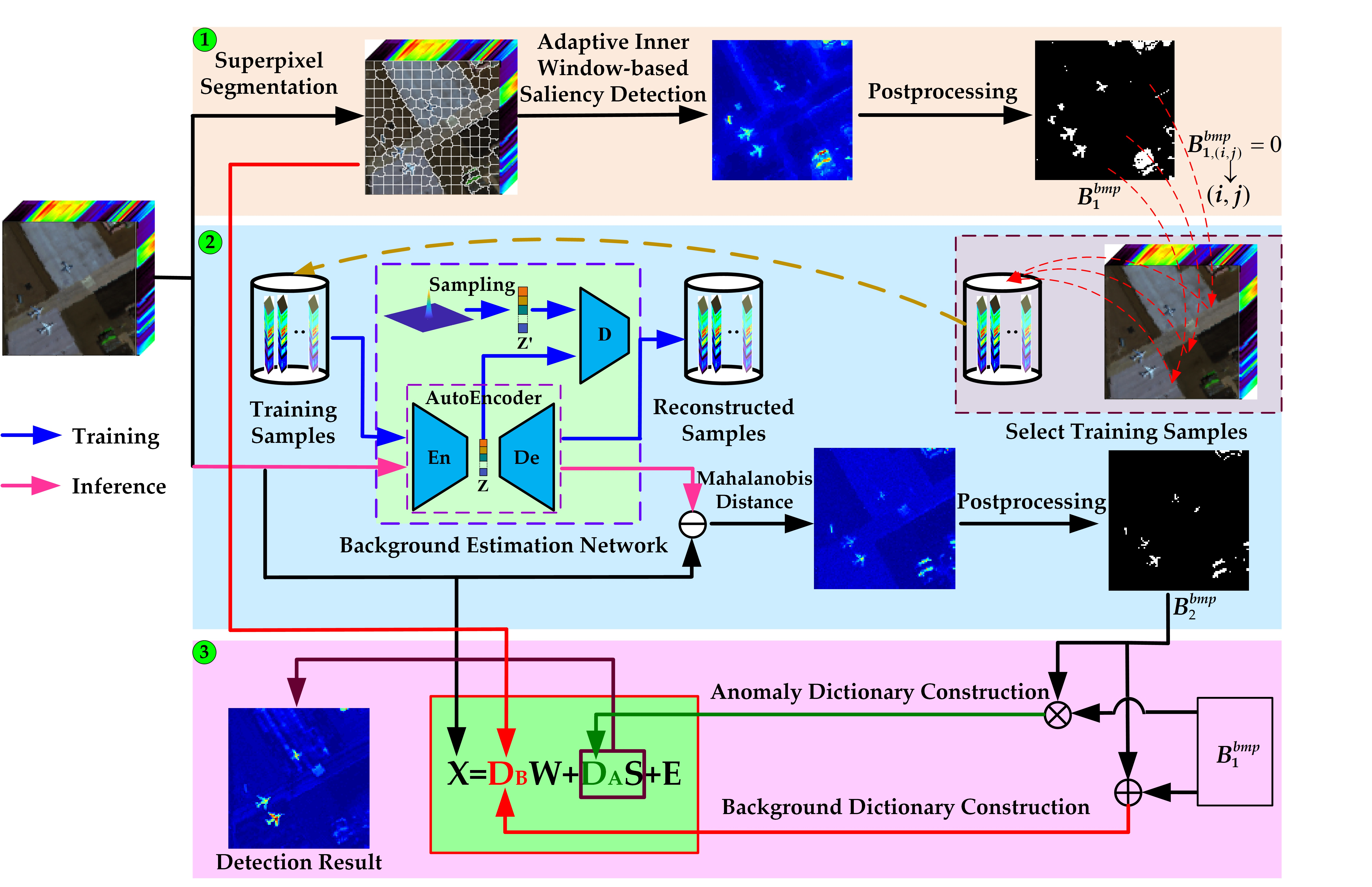
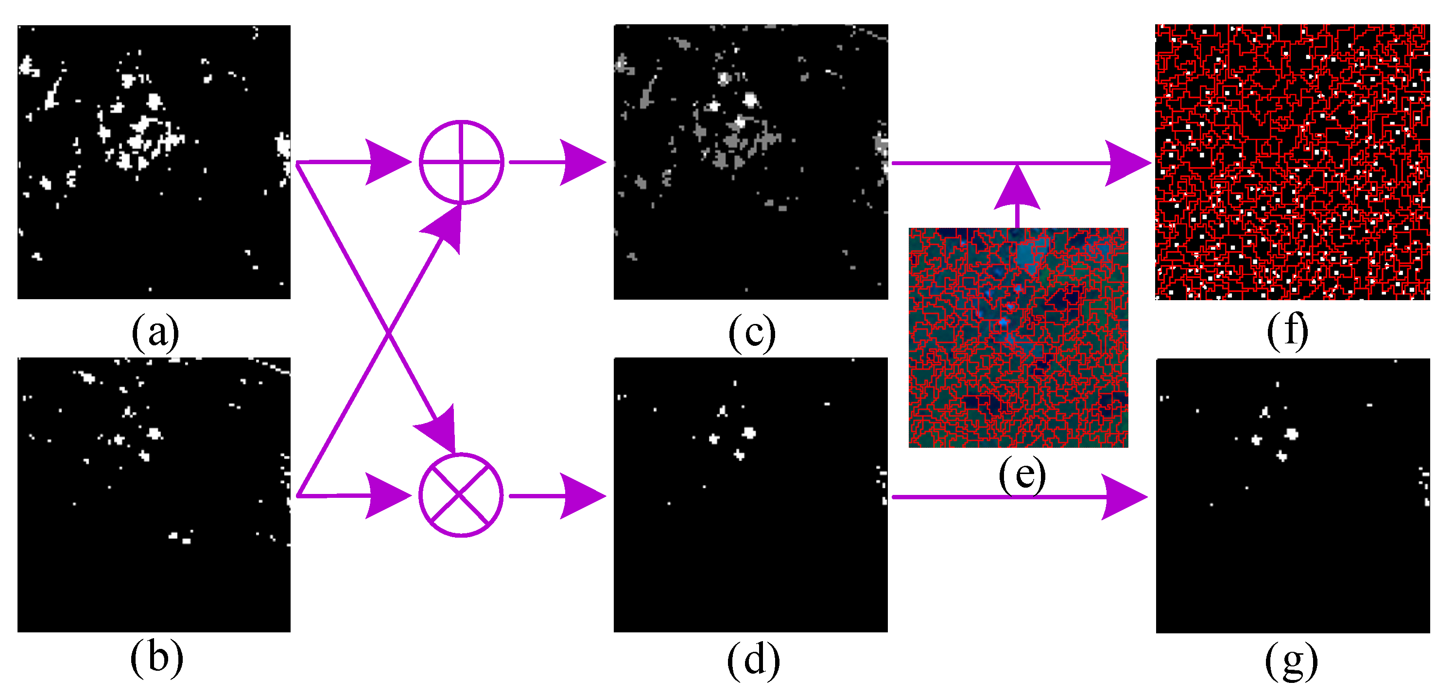
A novel dual dictionaries construction method via two-stage complementary decision, to the best of our knowledge, is first proposed to construct pure background and potential anomaly dictionaries in this paper. To be specific, the product of both coarse and fine binary maps acts as the indicator to sift anomalous pixels, and the sum of them is employed to assist in selecting background pixels.
(2)
A coarse background–anomaly separation strategy, which detects anomalies by performing the adaptive inner window–based saliency detection, is proposed to generate a coarse binary map. For the saliency detection, the key is that the superpixels act as the inner windows, which can effectively alleviate the situation that the testing pixel is affected by the pixels with similar characteristics distributed in the area between the inner and outer windows.
(3)
To obtain a fine binary map, a background estimation network, which consists of AE and GAN, is designed to acquire a strong background reconstruction ability and poor anomaly reconstruction effect.
(4)
To reduce the number of atoms in the background dictionary, the superpixels are employed to act as the auxiliary indicator to select the atoms in the construction of the background dictionary.
The remainder of this paper is organized as follows. Section 2 presents the related work. The proposed method is detailed in Section 3. Section 4 introduces the experiments and results. In Section 5, the discussion is given. Finally, the conclusions are drawn in Section 6.

2. Related Work

HAD has attracted increasing attention from researchers. Among all HAD methods, the RX detector [20], proposed by Reed-Xiaoli, is the most classical method. The RX algorithm assumes that the background obeys the multivariate Gaussian distribution; it establishes a background statistical model via calculating the mean value and covariance matrix of all pixels in HSI and then computes the Mahalanobis distance between the pixel under test and the background model to measure anomaly. Subsequently, instead of the global statistics leveraged in original RX, the variant of the RX, termed as Local RX (LRX) [21], utilizes the local statistics to construct the background model. Additionally, a lot of variants based on the RX detector, such as weighted RX (WRX) [22], kernel RX (KRX) [23] and fractional Fourier entropy RX (FrFERX) [24], are proposed to improve the detection performance of HAD. However, it is difficult to accurately model the background, due to the fact that the background is contaminated by the anomalies and noise to a certain extent.
To accurately model the background as much as possible, the representation-based methods, which consist of the collaborative representation-based methods (CR); the sparse representation-based methods (SR); and the low-rank-representation-based methods (LRR) are widely introduced into HAD. The classical CR detector (CRD) is proposed by Li et al. [25], assuming that the pixels belonging to the background can be linearly represented by its neighborhood pixels via a sliding windows, while anomalous pixels are not. The background joint sparse representation method (BJSR), which is a meaningful research based on the SR method, estimates the background through sifting the representative bases of all local regions [26]. The LRR-based methods consider that the background has a low rank property and the anomalies are sparse. With this condition, Zhang et al. [27] proposed the low rank and sparse matrix decomposition (LSMAD) to construct the background model via leveraging the low-rank characteristics of background excluding anomalies. Furthermore, constructing a background dictionary instead of background has been popularly adopted in HAD [28]. To characterize complex distribution, Li et al. [29] proposed the low rank and sparse decomposition model with mixture of Gaussian (LSDM–MoG), which models the sparse component as a mixture of Gaussian, to detect anomalies in HSIs. To fully use the local geometrical structure and spatial relationships, Cheng et al. [30] proposed the graph and total variation regularized low-rank representation-based detector (GTVLRR) for HAD. In the above LRR-based methods, the key is to construct a pure and comprehensive background dictionary, which is beneficial to improve the detection performance. Nevertheless, the background dictionary constructed by traditional methods has a limited capability to characterize the real complex background.
With the rapid development of deep learning [31,32,33], the deep-learning-based methods are extensively applied to HAD, due to its powerful capability to learn complex data distribution. Li et al. [34] attempted to transfer the deep convolutional neural network (CNN) into HAD. Specifically, a well-designed multilayer CNN is trained by using the spectral differences of paired samples derived from the reference data, and then the neighboring spectral differences between pixel pairs constructed by the pixel under test and its surrounding pixels are classified through the trained CNN, with the results of similarity measurement, and the output belonging to the pixel under test is achieved through averaging these similarity results. Subsequently, CNN-based algorithms, such as the transferred CNN based on tensor (TCNNT) [35] and autonomous hyperspectral anomaly detection network (Auto-AD) [36], are proposed for HAD. Additionally, the AE-based methods have attracted considerable attention, due to their powerful reconstruction ability. Zhao et al. [37] proposed a spectral–spatial stacked AEs based on low-rank and sparse matrix decomposition for HAD. Furthermore, deep generative models, including variation AE (VAE) [38] and generative adversarial network (GAN) [39], make significant contributions to HAD. Typically, the combination of AE and GAN is widely employed for HAD, such as unsupervised discriminative reconstruction constrained GAN for HAD (HADGAN) [40], semi-supervised spectral learning GAN (SSL-GAN) [41] and weakly supervised low-rank representation (WSLRR) [42]. However, the aforementioned methods generally fail to fully use two-stage information, resulting in limited detection performance.

3. Methodology

In this section, a detailed introduction of the proposed method is given as follows. Let X o h × w × b represent the original HSI, in which h and w are the height and width, respectively, and b denotes the number of spectral bands. In the following statement, the 3D cube X o h × w × b is converted into a 2D matrix X b × N , where N = h × w is the number of the pixels of the whole HSI. For HSIs, the background is generally viewed as low rank, due to the fact that each background pixel can be linearly represented by some background endmembers [43]. The anomalies appear in the HSIs with low probability and account for only a very small part of the entire image scene, indicating that the anomalies have sparse property [27]. Additionally, the noise always corrupts HSIs in practice; thus, it could not be ignored. Based on above analysis, we formulate the HAD task as a matrix decomposition problem in this paper. The HSI can be decomposed into three components: background with low-rank property, anomaly with sparse property and noise, which are expressed as follows:
X = B + A + E
where B b × N , A b × N and E b × N are the background component, anomaly component and noise component, respectively.
Considering that the background pixels are highly correlated, which means that each of them can be linearly represented by some background pixels. Similarly, the anomalous pixels are proved to be correlated to a certain extent [43]. As a result, the decomposition of the HSI can be reformulated as
X = D B W + D A S + E
where D B W and D A S are the low-rank component and sparse component, respectively; D B = { d b i b × 1 } i = 1 m and D A = { d a i b × 1 } i = 1 n are background and potential anomaly dictionaries matrices, respectively; m and n separately represent the number of atoms in the background and potential anomaly dictionaries; and W = { w i m × 1 } i = 1 N and S = { s i n × 1 } i = 1 N indicate the representation coefficient corresponding to the background and anomaly components, respectively.
To model the problem (2), an objective function is formulated as follows:
min W , S , E W + β S 1 + λ E 2 , 1 s . t .   X = D B W + D A S + E
where ||·||*, ||·||1 and ||·||2,1 represent the nuclear norm, l1 norm and l2,1 norm, respectively. β and λ are the coefficients to balance the sparse and noise terms, respectively.

3.1. Coarse Background–Anomaly Separation

The coarse background–anomaly separation (CBAS) involves generating a coarse binary map, which is of significant importance for subsequent procedures. On the one hand, the coarse binary map is employed as the indicator to select the training samples (i.e., background pixels). On the other hand, the coarse binary map guides the construction of background and potential anomaly dictionaries. The procedure of CBAS is roughly subdivided into three key steps: superpixel segmentation, adaptive inner window–based saliency detection and post-processing, as illustrated in Figure 2. The details can be described as follows.

3.1.1. Superpixel Segmentation

Superpixel is a collection of adjacent pixels which are of similar color, texture and other characteristics [44]. In the existing superpixel segmentation methods, the simple linear iterative clustering (SLIC) [45] algorithm has attracted widespread concern, due to the characteristics of fast speed, high memory efficiency and excellent boundary adherence. To this end, a SLIC-based superpixel segmentation method, which was extended from RGB images to HSIs, was employed in this study. The SLIC method is reckoned as the generalization version of the k-means clustering algorithm to some extent. In contrast to the k-means clustering algorithm, the SLIC method merges the pixels with similar characteristics in a local region rather than global scope. To be specific, the preset number (i.e., K) of superpixels with approximately equal size is first determined, and the center point of each superpixel acts as the initial cluster center. Then the distance between the cluster center and pixels distributed in its local region (i.e., 2s × 2s, s = N / K ) is calculated. Considering the cluster center, x c , with spatial coordinate ( x c , y c ) and neighborhood pixel, x i , with spatial coordinate ( x i , y i ) , the distance metric containing spatial distance and spectral distance is defined as follows:
d s p a ( x c , x i ) = ( x c x i ) 2 + ( y c y i ) 2 / 2 s
d s p e ( x c , x i ) = cos 1 ( < x c , x i > x c · x i )
d ( x c , x i ) = ω × d s p a + ( 1 ω ) × d s p e
where d s p a , d s p e and d are the spatial distance, spectral distance and total distance, respectively; < · , · > denotes the inner product of two spectral vector; · indicates the norm of the spectral vector; and ω represents the tradeoff parameter for balancing the spatial distance and spectral distance.
After that, the centers of all superpixels will be updated according to the above distance metric. Until the centers of all superpixels no longer update, the final superpixels are formed.

3.1.2. Adaptive Inner Window–Based Saliency Detection

For HSIs, the anomalous pixel has significant spectral difference relative to its surrounding pixels. In human vision system, a target that is focused on at first glance is viewed as significant [16]. In other words, one part in an image that is first noticed is treated as salient. For the above reasons, the saliency detection can act as an effective technique to perform HAD.
The context-aware saliency detection (CaSD) method, proposed by Goferman et al. [17], is an effective approach to detect the salient regions of an image, and it follows the fact that the salient objects are strongly distinctive with both local and global surroundings. In the existing CaSD methods [15,46] utilized in HAD, the saliency-detection result commonly acts as the saliency weight for suppressing the background and highlighting the anomalies. Additionally, the implementation of the saliency detection is by means of the dual rectangular windows; however, the anomalous pixel under test is possibly similar to the pixels distributed in the interval of inner and outer windows, leading to a low contrast (i.e., a low saliency value), as shown in Figure 3a. In Figure 3a, the green rectangular box and red rectangular box are the inner window and outer window of the pixel under test (i.e., small blue rectangular box), respectively. By observing Figure 3a, we can see that some pixels distributed in the area between the inner and outer windows are similar to the pixel under test, and this will affect the result of the saliency detection.
To resolve the above issue, we propose an adaptive inner window–based saliency detection method in this paper. Concretely, instead of applying dual rectangular windows, we took advantage of superpixel segmentation to yield a flurry of homogeneous regions with similar characteristics, which were employed as the inner window to perform saliency detection, as illustrated in Figure 3b. In Figure 3b, the irregular polygon in green and rectangular box in red separately represent the adaptive inner window and outer window, and the purple dashed box refers to the smallest enclosed rectangular box covering an irregular polygon, which is used to determine the outer window with distance R. Note that the small blue rectangular boxes in Figure 3a,b represent pixels at the same location. Evidently, for the same pixel under test, it can see in Figure 3b that there are few pixels which are similar to the anomalous pixel under test between the inner and outer windows, and this is beneficial to the detection performance. In this way, the anomalous pixels appear in the area between inner and outer windows with a low probability, and, hence, the anomalous pixel under test have a high contrast (i.e., a high saliency value). In addition, we directly employed the saliency detection result to determine the probability of anomaly, rather than as a saliency weight. It is worth noting that the adaptive inner window–based saliency detection shares the same inner window and outer window for the pixels located in the same superpixel, while the dual rectangular windows–based saliency detection employs a unique inner window, R i n n e r , and outer window, R o u t e r , for each pixel.
According to above analysis, let y indicate the pixel under test, assuming it is inside the green irregular polygon in Figure 3b, and let x t represent the pixel distributed in the area between the inner window and outer window (i.e., inside the red rectangular box and outside the green irregular polygon in Figure 3b). The adaptive inner window–based saliency detection can be calculated as follows:
d s a l t ( x t , y ) = d s p e ( x t , y ) 1 + c · d p o s ( x t , y )
where d s p e ( x t , y ) and d p o s ( x t , y ) are separately the spectral distance and position distance between the spectral vector x t and y ; and c is a constant, which has little influence on the result, and, hence, it is set to 1 for convenience.
d s p e ( x t , y ) = cos 1 ( < x t , y > x t · y )
d p o s ( x t , y ) = ( x t r y r ) 2 + ( x t c y c ) 2
where ( x t r , x t c ) and ( y r , y c ) indicate the spatial coordinates of the pixels x t and y , respectively. Once all pixels distributed in the area between the inner window and outer window have participated in the saliency detection of the testing pixel, we take the average of all saliency values and make it a final saliency result, which can be defined by the following equation:
d s a l a v g = Σ t = 1 S d s a l t S
where S denotes the number of pixels in the area between the inner window and outer window of the testing pixel. Through the above way, an anomaly map, d 1 , can be obtained.

3.1.3. Post-Processing

To generate a coarse binary map, a post-processing operation, which consists of thresholding and area filtering, is imposed on the anomaly map, d 1 . A simple yet effect method, which uses the OTSU algorithm [47] to threshold potential anomaly map, is firstly adopted. The binary map, B, can be acquired through the following formula:
B = t h r e s h o l d ( d 1 ; ε )
where the function t h r e s h o l d ( · ; ε ) assigns 1 to a pixel if its value exceeds the threshold ε ; if otherwise, it is 0. Moreover, ε is obtained through the OTSU algorithm [47], owing to the excellent performance in image binarization.
It is worth noting that a background object occupying voluminous pixels is possibly reckoned an anomaly. To tackle this issue, a suppression strategy, which removes the connected domain with large areas in the guidance of the binary map, is performed, which is processed as follows:
B 1 b m p = A R E A _ F I L T E R I N G ( B ; τ )
where the function A R E A _ F I L T E R I N G ( · ; τ ) assigns 0 to the connected domain if the connected domain larger than the specified threshold, τ . Generally speaking, the higher the τ , the less the removed components. With this situation, the large background object is retained, which fails to choose background pixels as much as possible. Conversely, the smaller the τ, the more the removed components. In this way, the anomalies with a large area are possibly removed, and it is harmful to sift the background pixels in the following step, due to the contamination of the anomalous pixels. Therefore, in this study, we set τ to be N/100, where N is the number of pixels in HSI. Through the above method, a coarse binary map, B 1 b m p , is obtained.

3.2. Fine Background–Anomaly Separation

In this part, we recount how a background estimation network (BEN), which consists of three subnetworks (i.e., encoder network, decoder network and discriminator network), was constructed. The purpose of constructing the BEN was to learn an evaluator for judging the probability of a pixel being an anomaly. The coarse binary map, B 1 b m p , was used for sifting the background pixels, and the selection strategy is shown as follows:
C B = { x ( i 1 ) · w + j | B 1 , ( i , j ) b m p = 0 ( i , j ) , i [ 1 , h ] , j [ 1 , w ] }
where C B b × S b represents the collection of the selected background pixels, in which S b indicates the number of the selected background pixels, and b denotes the number of bands in HSI; x ( i 1 ) · w + j b × 1 is the pixel in row i and column j in HSI. The details of the fine background–anomaly separation are given in the following.

3.2.1. Network Architecture

Generally speaking, the anomalous pixels only account for a small part relative to the background pixels in HSIs [28]. Based on the above fact, we take advantage of the autoencoder (AE) with powerful reconstruction ability to act as a basic model of BEN, which is beneficial to learn strong background reconstruction capability and poor anomaly reconstruction ability, due to the strictly imbalanced distribution of background and anomaly in HSIs. Furthermore, in order to improve the background reconstruction capability, an adversarial strategy was introduced into the AE. In this situation, a BEN, illustrated in Figure 2, which is composed of AE and adversarial module, was formed.
An AE is a feed-forward neural network containing an encoder and a decoder. The parameters of AE, including weight and bias, are updated by using the back-propagation method [48]. The encoder is utilized to learn a mapping from the input data, x , to the latent feature, z , and the decoder maps from the latent feature ( z ) to the reconstructed data, x ^ . The whole mapping process is summarized as follows:
z = f e n ( ω e n x + b e n )
x ^ = f d e ( ω d e z + b d e )
where f e n ( · ) and f d e ( · ) are the mapping function of encoder and the mapping function of decoder, respectively; and ω e n and b e n separately symbolize the weight and bias of encoder. Similarly, ω d e and b d e signify the weight and bias of decoder, respectively.
After an AE is formed, an adversarial strategy that involves introducing a discriminator subnetwork is adopted in AE. Here, the encoder and the discriminator subnetwork jointly make up a generative adversarial network (GAN), and its core idea is generating new data points with some variations via learning specific data distributions in a min-max game way. The GAN contains two adversarial components, a generator, G, and a discriminator, D, in which the encoder acts as the generator (G). The generator (G) strives to map the input data ( x ) to the latent feature ( z ), which is as close as possible to the real data ( z ) sampling from the prior distribution, N ( 0 , I ) . Subsequently, two samples, namely the real data ( z ) and fake data ( z ) (i.e., latent feature z ) are fed into the discriminator (D), which attempts to distinguish which of the two are the real data and gives the corresponding confidence. In other words, the generator tries to fool the discriminator, and the discriminator strives to discern the real or fake of the input in an adversarial manner.

3.2.2. Training Process

In the training stage, the selected background pixels collection, C B , was used to discriminatively train the BEN, which is beneficial to learn the background reconstruction ability without contamination of the anomalous pixels. The objective loss of BEN, which contains the joint objective loss of AE and GAN, is expressed as follows:
L = L A E + α · L G A N
L A E = 1 b x b a c x ^ b a c 2
L G A N = min E n max D E z N ( 0 , I ) [ log D ( z ) ] + E x b a c p d a t a [ log ( 1 D ( E n ( x b a c ) ) ) ]
where L A E and L G A N separately represent objective the loss of AE and GAN; α denotes the tradeoff coefficient to balance L A E and L G A N , for which we empirically set it to 1 for the optimal result; x b a c and x ^ b a c are the input background spectral vector and reconstructed background spectral vector, respectively; E n ( · ) and D ( · ) represent the encoding operation and discrimination operation, respectively; and p d a t a stands for the distribution of the selected background pixels. Here, z and E n ( x b a c ) strive to gain D’s preference; in this way, D intends to maximize the L G A N , while E n does the opposite.

3.2.3. Anomaly Detection on Residual HSI

In this stage, the original HSI X = [ x 1 , x 2 ,   , x N ] b × N was first fed into trained BEN and then obtained the reconstructed HSI X ^ = [ x ^ 1 , x ^ 2 , , x ^ N ] b × N , in which the background pixels were well reconstructed while the reconstruction of anomalous pixels was poor, as illustrated in Figure 4. Therefore, the residual HSI X R = [ x r 1 , x r 2 ,   , x r N ] b × N between the original HSI and reconstructed HSI can highlight the anomaly and suppress the background. In this way, we employed the residual HSI to detect anomalies via applying the Mahalanobis distance, which can be expressed as follows:
d 2 , i = ( x r i μ ) T Σ 1 ( x r i μ ) ,   i [ 1 , N ]
where d 2 , i represents the detection result of the ith pixel in HSI; and μ b × 1 and Σ b × b are the mean vector and covariance matrix of the residual HSI X R , respectively. Different from directly applying the Mahalanobis distance on original HSI, the residual HSI has a more discriminative characteristic in regard to the background and anomaly, and this is helpful to detect the anomalies.
After the detection map, d 2 = [ d 2 , 1 , d 2 , 2 , , d 2 , N ] was obtained; the detection map, d 2 , was first converted into the 2D matrix; and then the same post-processing operation was used as was discussed in Section 3.1.3 to deal with the 2D matrix for acquiring a fine binary map B 2 b m p .

3.3. Dual-Dictionaries-Based Low Rank and Sparse Representation

3.3.1. Dual Dictionaries Construction

Generally speaking, anomalies with a strong spectral difference relative to the background can be used as a potential prior to represent the other anomalies [19]. Motivated by this, we considered mining the potential anomalies in HSIs. Obviously, the potential anomalies can be easily detected in Section 3.1 and Section 3.2, meaning that the combination of both can be an effective manner to construct the background and potential anomaly dictionaries. Toward this goal, the product of two binary maps can act as a prior to construct a potential anomaly dictionary for detecting the other anomalies. Similarly, the sum of two binary maps can easily be considered to construct a background dictionary. In this way, there are few background pixels contamination in the construction of the potential anomaly dictionary; this can guarantee the purity of atoms in the potential anomaly dictionary.
Based on above analysis, we employed two binary maps (i.e., B 1 b m p and B 2 b m p ) to jointly construct the background and potential anomaly dictionaries. Concretely, the index maps, acting as the indicator for constructing background and potential anomaly dictionaries, were first obtained by the addition operation and multiplication operation pixel by pixel, respectively, which are formulated as follows:
B m = B 1 b m p B 2 b m p
A m = B 1 b m p B 2 b m p
where B m h × w and A m h × w are index maps for sifting background pixels and anomalous pixels, respectively; and and represent the addition and multiplication operations pixel by pixel, respectively.
Once B m and A m are obtained, the element in B m whose value is “0” can be considered to guide the selection of the atoms in the construction of the background dictionary; however, this results in high computation complexity for the optimization of LRSR. To reduce the number of atoms in the background dictionary, the superpixels and B m are jointly utilized to guide the selection of atoms in the construction of the background dictionary. Similarly, A m is considered to assist in the construction of the potential anomaly dictionary. Specifically, if an area belonging to B m with an identical position to a superpixel contains the elements whose values are all “0”, the corresponding superpixel will participate in the construction of the background dictionary; otherwise, it will not. It is worth noting that only the centroids of the selected superpixels act as the atom to form the background dictionary in the consideration of the effectiveness and computation complexity. Different from the above, the element whose value is “1” in A m is selected to act as the atom to construct the potential anomaly dictionary. The details can be expressed as follows:
D B = { x s k | B S k m = 0 k } , k [ 1 , K * ]
D A = { x ( i 1 ) · w + j | A i , j m = 1 ( i , j ) } , i [ 1 , h ] , j [ 1 , w ]
where D B and D A represent the background and potential anomalies dictionaries, respectively; B S k m denotes the sum of B m with the same position as the kth superpixel; A i , j m { 0 , 1 } is the element at position ( i , j ) in A m ; K * is the number of the superpixels; and x s k indicates the spectral vector corresponding to the centroid of the kth superpixel. To better understand the construction process of background and potential anomaly dictionaries, an example is given in Figure 5.

3.3.2. Low Rank and Sparse Representation

As stated at the beginning of Section 3, the HAD task was reckoned as a matrix decomposition problem, and it was transformed into Equation (3). With D B and D A constructed in Section 3.3.1, to solve the LRSR problem as (3), two auxiliary variables, J and L, are introduced to make the objective function separable. Consequently, the problem of (3) can be converted into the following form:
min W ,   S ,   E ,   J ,   L J + β L 1 + λ E 2 , 1 s . t . X = D B W + D A S + E , W = J , S = L
The augmented Lagrange function of problem (24) is as follows:
l = J + β L 1 + λ E 2 , 1 +   tr [ Y 1 T ( X D B W D A S E ) ] + tr [ Y 2 T ( W J ) ] + tr [ Y 3 T ( S L ) ] + μ 2 ( X D B W D A S E F 2 + W J F 2 + S L F 2 )
where Y1, Y2 and Y3 are the Lagrange multipliers; μ is a penalty parameter; and tr[·] refers to the trace of a matrix. The problem (25) can be solved with the alternating direction method of multipliers (ADMMs) method [49], of which the core idea of this is to fix other variables while updating one variable.
(1)
Update J while fixing L, E, W and S. The objective function can be derived as follows:
min J J + μ 2 J ( W + Y 2 μ ) F 2
(2)
Update L while fixing J, E, W and S. The objective function can be derived as follows:
min L β L 1 + μ 2 L ( S + Y 3 μ ) F 2
(3)
Update E while fixing J, L, W and S. The objective function can be derived as follows:
min E λ E 2 , 1 + μ 2 E ( X D B W D A S + Y 1 μ ) F 2
(4)
Update W while fixing J, L, E and S. The objective function can be derived as follows:
min W   < Y 1 , X D B W D A S E > + < Y 2 , W J > + μ 2 ( X D B W D A S E F 2 + W J F 2 )
(5)
Update S while fixing J, L, E and W. The objective function can be derived as follows:
min S < Y 1 , X D B W D A S E > + < Y 3 , S L > + μ 2 ( X D B W D A S E F 2 + S L F 2 )
The solution of the optimization process is outlined in Algorithm 1. Note that the Φ , Ω and Θ used in Algorithm 1 separately refer to the singular value thresholding [50], soft thresholding [51] and l2,1 norm minimization operator [28].
Algorithm 1. Solve (25) by ADMM.
Input: HSI   X = { x i } i = 1 i = N b × N , balance parameter λ and β.
Initialize: W = J = S = L = 0, E = 0, Y1 = Y2 = Y3 = 0, μ = 10−6, μmax = 1010, ρ = 1.2, ε = 10−6.
1: While max ( X D B W D A S E F , W J F , S L F ) ε do
2: Update J while fixing other variables by (26):
         J Φ 1 / μ ( W + Y 2 / μ )
3: Update L while fixing other variables by (27):
         L Ω β / μ ( S + Y 3 / μ )
4: Update E while fixing other variables by (28):
         E Θ λ / μ ( X D B W D A S + Y 1 / μ )
5: Update W while fixing other variables by (29):
         W ( D B T D B + I ) 1 [ D B T X D B T D A S D B T E + J + ( D B T Y 1 Y 2 ) / μ ]
6: Update S while fixing other variables by (30):
         S ( D A T D A + I ) 1 [ D A T X D A T D B W D A T E + L + ( D A T Y 1 Y 3 ) / μ ]
7: Update the three Lagrange multipliers:
         Y 1 Y 1 + μ ( X D B W D A S E )
         Y 2 Y 2 + μ ( W J )
         Y 3 Y 3 + μ ( S L )
8: Update the balance parameter μ :
         μ min ( ρ μ , μ max )
9: End While
Output: W, S, E
Once the optimization process is terminated, the detection result can be determined by the sparse component, D A S , as follows:
T ( x i ) = [ D A S ] : , i 2 = j = 1 b ( [ D A S ] j , i ) 2 , i [ 1 , N ]
where [ D A S ] : , i 2 represents the l2 norm of the ith column of D A S .

4. Experiments and Results

In this section, we recount how a large number of experiments were carried out to validate the effectiveness and superiority of the proposed method.

4.1. Datasets and Evaluation Metrics

4.1.1. Datasets

To verify the effect of the proposed method, five public datasets, including six HSIs with different characteristics, are introduced.
HYDICE dataset [52]: The first dataset, captured by the Hyperspectral Digital Imagery Collection Experiment (HYDICE) airborne sensor, covers an urban area of CA, USA. The dataset has 80 × 100 spatial pixels with 175 spectral bands, ranging from 400 to 2500 nm, and a 1-m spatial resolution. The anomalies consisting of 21 pixels are mainly cars and roofs. The color composites and corresponding reference map are displayed in Figure 6(I-a,I-b), respectively.
Pavia dataset [27]: The second dataset was acquired by the Reflective Optics System Imaging Spectrometer (ROSIS-03) sensor over the center of Pavia city in Northern Italy. The whole HSI contains 102 spectral bands, ranging from 430 to 860 nm, and each of them covers an area of 100 × 100 pixels, and its spatial resolution is 1.3 m. The vehicles on the bridge are viewed as the anomalies, accounting for 68 pixels in total in the image scene. The color composites and corresponding reference map are separately illustrated in Figure 6(II-a,II-b).
Los Angeles dataset [42]: The third dataset was collected by the Airborne Visible/Infrared Imaging Spectro-meter (AVIRIS) sensor over the Los Angeles city in USA. The image scene contains 100 × 100 pixels and 205 spectral bands spanning from 430 nm to 860 nm after removing corrupted bands. The spatial resolution of the HSI is 7.1 m, and the number of total anomalous pixels is 272, which are all buildings. The color composites and corresponding reference map are showed in Figure 6(III-a,III-b), respectively.
San Diego dataset [52]: The fourth dataset, including two HSIs with different characteristics, was captured by the AVIRIS sensor covering the area of San Diego airport, CA, USA. The pixels of two HSIs are 100 × 100 and 120 × 120, respectively, and the number of bands totals 189 on both HSIs, in a wavelength spanning from 400 to 2500 nm. The spatial resolutions of the HSIs are both 3.5 m. The airplanes separately occupying 134 and 58 pixels are viewed as anomalies to be detected for the two HSIs. The color composites and corresponding reference map of San Diego-I are shown in Figure 6(IV-a,IV-b), respectively. Similarly, Figure 6(V-a,V-b) show the corresponding color composites and reference map for San Diego-II.
Texas Coast dataset [53]: The fifth dataset covering the Texas Coast area was obtained by the AVIRIS sensor with 17.2 m spatial resolution. The whole HSI contains 204 spectral bands, ranging from 450 to 1350 nm, and each of them is 100 × 100 pixels. The anomalies (i.e., buildings) embedded in the background contain 67 pixels in total. The color composites and corresponding reference map are exhibited in Figure 6(VI-a,VI-b).

4.1.2. Evaluation Metrics

To measure the detection results, three commonly used evaluation criteria, which are separately the receiver operating characteristic (ROC) curve [54], the area under the curve (AUC) [55] and the separability range [56], were introduced into HAD. The ROC curve depicts the true-positive rate (Pd) versus the false-positive rate (Pf) corresponding to various thresholds. For the ROC curve, the better the performance, the higher the curve. Corresponding to the ROC curve, the AUC value was adopted. Theoretically, an outstanding anomaly detector should have a larger AUC value that approaches 1. The separability range generated from the boxplot characterizes the capability of the detector to extract anomalies from the background. The boxplot displays the variation in samples of a statistical population, which is nonparametric, without any assumption of the underlying statistical distribution. The degree of dispersion and skewness in the data can be described by the spacings between the different parts of the box. A better detector should have a more obvious separation between the anomalies and background.

4.2. Experimental Setup

4.2.1. Implementation Details

The background estimation network (BEN) introduced in Section 3.2 contains three subnetworks, in which each of them consists of four fully connected layers, and the number of nodes over all subnetworks are respectively defined to E n { b , 512 , 512 , N z } , D e { N z , 512 , 512 , b } , D { N z , 512 , 512 , 1 } . Here, b represents the spectral dimension of input HSIs, and N z stands for the dimension of latent feature, which is empirically determined by Reference [40]. The Leaky ReLU with slope 0.2 acts as the activation function after each fully connected layer in all subnetworks. Considering the limitation of the number of training samples, a dropout strategy [57] with a sampling rate of 0.5 is introduced into BEN to prevent overfitting. For the discriminator network, a sigmoid function is imposed on the last layer to constrain the output to [0, 1]. The batch size of BEN in training stage is set to the number of the training samples, and the iteration epoch is set to 1000. The learning rate of AE and discriminator are separately 1 × 10⁻³ and 1 × 10⁻⁴, and the corresponding optimizers are both Adam [58]. Additionally, the tradeoff parameter, ω , for weighing the spectral and spatial distances in superpixel segmentation is set to 0.3 [59]. The above hyperparameters were the default in our experiments, and the user can tune these hyperparameters for optimal results.
The experiments using our method were carried out on a running environment with Python 3.6.13, Pytorch-gpu 1.8.2 and CUDA 10.2 by using GeForce RTX 2080Ti graphics card. All comparative methods, except for PAB-DC, were executed by using MATLAB R2017b on an Intel(R) Core(TM) i7-9700T CPU 2.00GHz machine with 16GB of RAM. Similarly, PAB-DC was also performed on a running environment with Python 3.6.13.

4.2.2. Compared Methods

To verify the performance of the proposed method, seven widely used methods, which contain four typical methods and three state-of-the-art methods, were employed for comparison. The first typical method is the RX detector [20], which is the benchmark of the statistical-based methods. The remaining three typical methods are the representation-based methods, including the collaborative representation-based method (i.e., CRD [25]), the low rank and sparse matrix decomposition–based method (i.e., LSMAD [27]) and the low rank and sparse representation–based method (i.e., LRASR [28]). The three state-of-the-art methods consisting of PAB-DC [19], LSDM–MoG [29] and KIFD [52] were proposed recently.

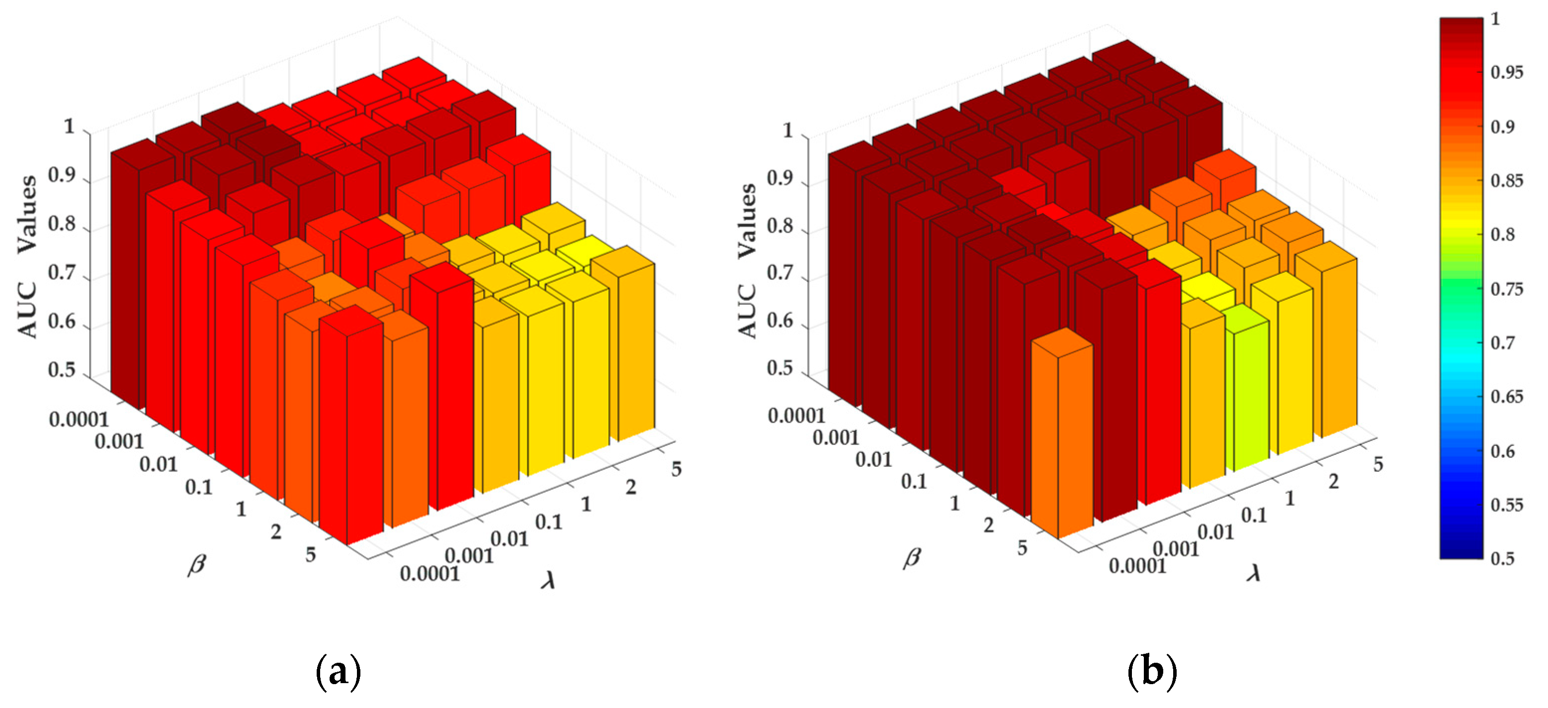
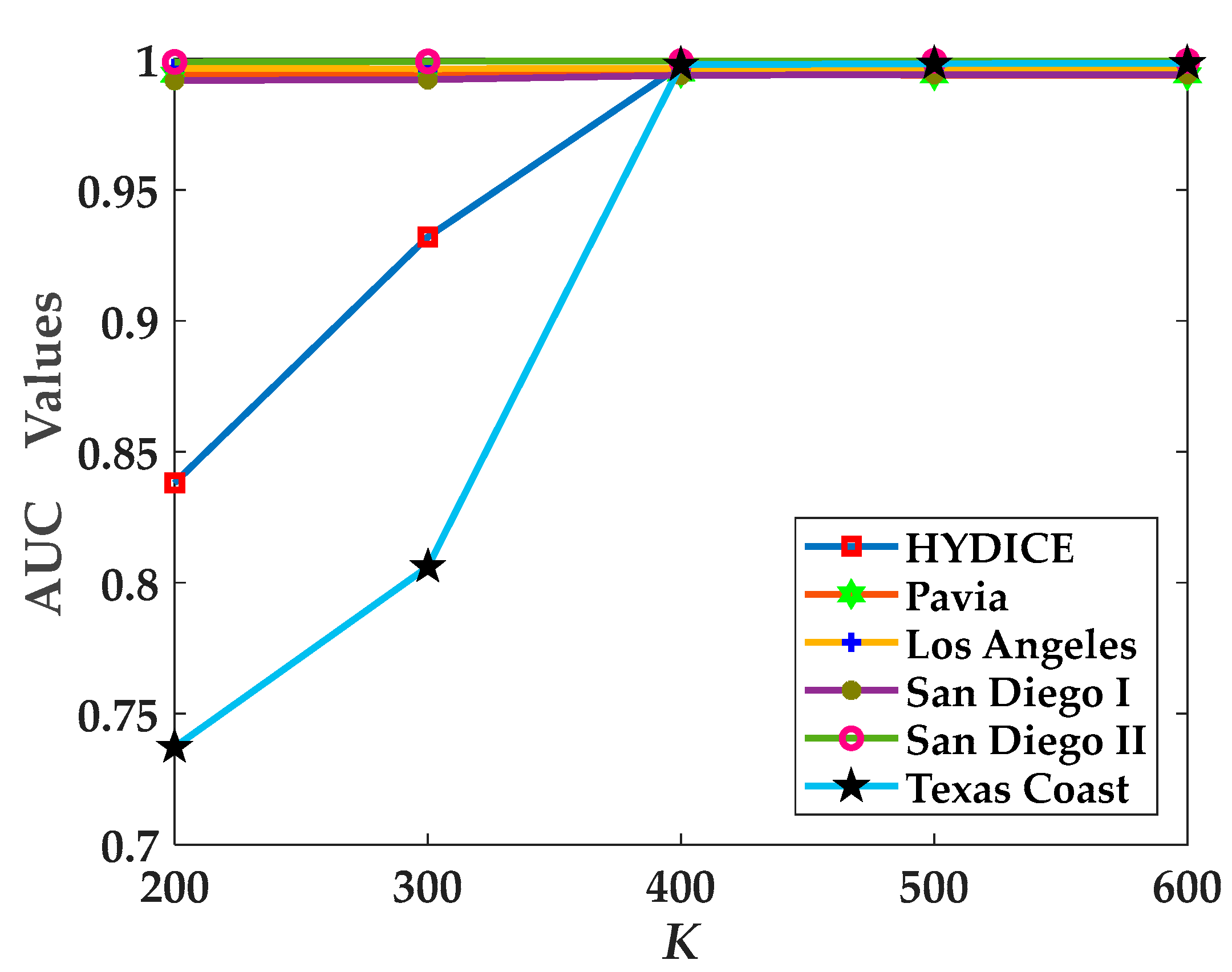
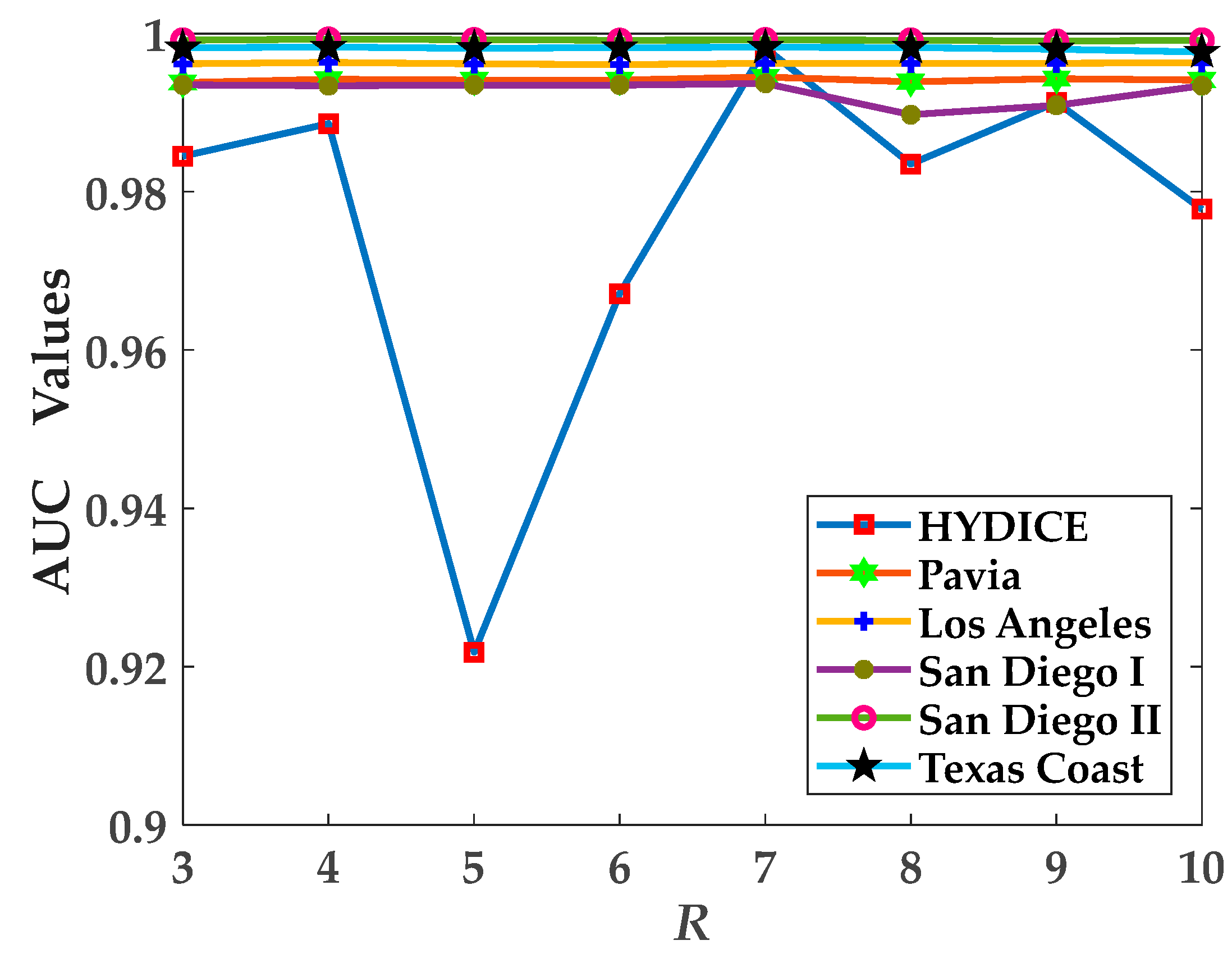
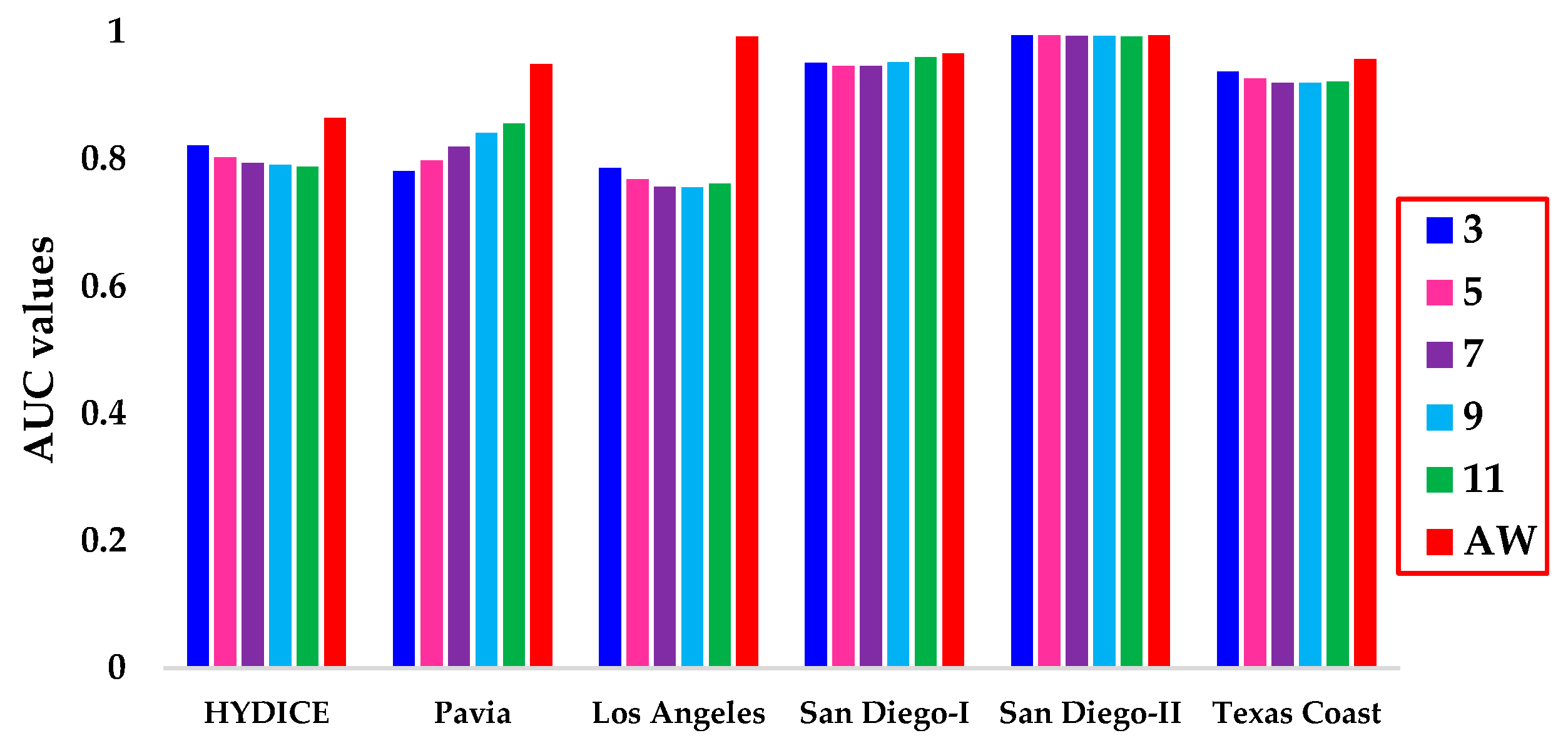
4.3. Parameter Analysis

With the above configured hyperparameters described in Section 4.2.1, there four are remaining parameters to be considered that are, respectively, the number of the preset superpixel, K, in Section 3.1.1; the distance, R, between inner and outer windows in Section 3.1.2; and the tradeoff parameters, λ and β, in Equation (24). When K is relatively small, there are few participants in the background dictionary, and this is harmful to detection performance. Inversely, the computation complexity of LRSR will be very high when K is quite large. As shown in Figure 7, to balance both aspects mentioned above, K is set to a reasonable range, i.e., {200, 300, 400, 500, 600}. By observing Figure 7, we can see that K has little influence on AUC value for the experimental datasets, except for the HYDICE and Texas Coast datasets, and the proposed method achieves optimal results when K is 400. In terms of R, the larger the R, the more complex the computation. In contrast, the detection result is vulnerable to the R when R is relatively small. To this end, by considering the above conditions, a group of numbers, which range from 3 to 10 at an interval of 1, are set to analyze influence of R over the AUC value on the experimental datasets, as illustrated in Figure 8. It can be seen that there is a significant fluctuation over the AUC value on the HYDICE dataset with the increase of R, and it achieves a first-rank performance when R is equal to 7. Relative to the dramatic change in the HYDICE dataset, the AUC values for other datasets remain stable and at a high level. Additionally, we consider both the tradeoff parameters, λ and β, together. Here, both λ and β are chosen from {0.0001, 0.001, 0.01, 0.1, 1, 2, 5}, which is similar to PAB-DC [19]. As shown in Figure 9, taking the Pavia and Los Angeles datasets for example, two 3D histograms are displayed to explore the effect of λ and β over the AUC value. To acquire optimal detection results, extensive experiments were conducted for each dataset, and corresponding best results are listed in Table 1.

4.4. Component Analysis

4.4.1. Effectiveness Evaluation of Adaptive Inner Window–Based Saliency Detection

To validate the effect of the adaptive inner window–based saliency detection, we compared it with the dual rectangular windows–based saliency detection. Generally speaking, dual rectangular windows–based methods always set a group of inner and outer windows with different scales in an (Rin, Rout) way to search for the optimal result, whereas only the size R between the inner window and outer window can be adjusted manually in our method. For the above reason, for fair comparison, we ensure that the result of “RoutRin” is equal to R and adjust the size of inner window in the dual rectangular windows. Considering that the searching scope of the superpixel segmentation is 2s × 2s, we set a group of reasonable size for the inner window in the dual rectangular windows that ranges from 3 to 11 at an interval of 2, i.e., {3, 5, 7, 9, 11}. Taking R = 7 as an example, we conducted a series of experiments to evaluate the effectiveness of the proposed adaptive inner window–based saliency detection, and the AUC values are shown in Figure 10. By observing Figure 10, we can observe that the adaptive inner window–based saliency detection is superior to that of the dual rectangular windows–based detection on experimental datasets, except for the San Diego-II dataset. For San Diego-II, we can easily find that adaptive inner window–based method is comparable to the dual rectangular windows–based method. The main reason behind this is that the detection result is nearly close to 1, and thus the improvement is not obvious. In summary, the adaptive inner window–based saliency detection is a useful technique to detect the anomalies.

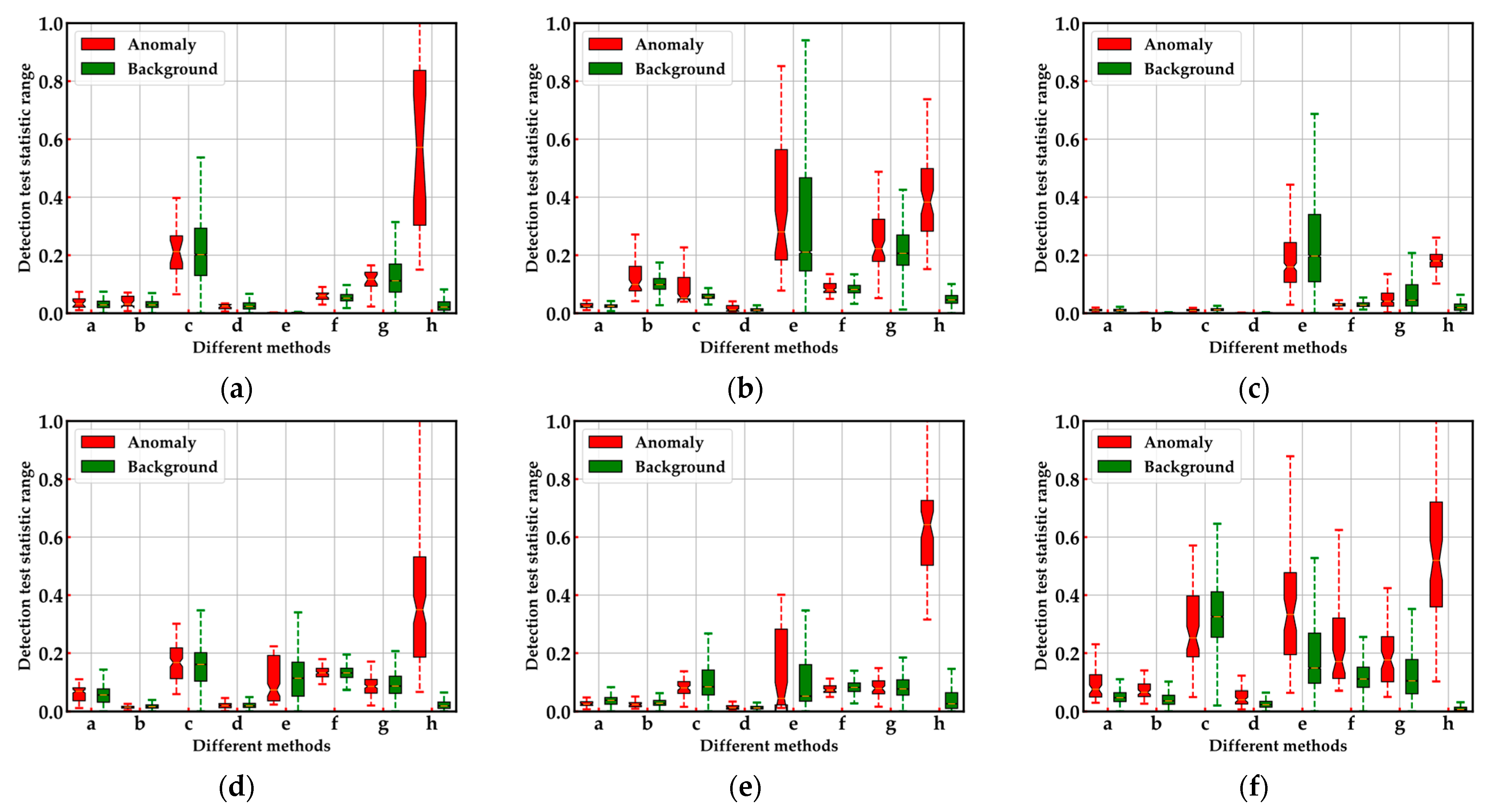
4.4.2. Effectiveness Evaluation of Two-Stage Complementary Decision

To validate the contribution of the proposed two-stage complementary decision for dual dictionaries construction, the dual dictionaries construction with only coarse binary map, dual dictionaries construction with only fine binary map and dual dictionaries construction with two-stage complementary decision were conducted on six HSIs for comparison, which are separately represented by “Coarse”, “Fine” and “Complementary” in Table 2. By observing Table 2, we can see that the “Complementary” achieves optimal AUC values on overall experimental datasets compared with “Coarse” and “Fine”. Taking the Los Angeles dataset for example, the visualization of the detection maps is displayed in Figure 11. Through Figure 11, it can be seen that some anomalies existed in “Coarse” and “Fine” are submerged into the background, and this is not conductive to observation, whereas the anomalies appeared in “Complementary” are almost highlighted. Therefore, the combination of coarse and fine binary maps was proven to be effective for detecting anomalies and suppressing background.

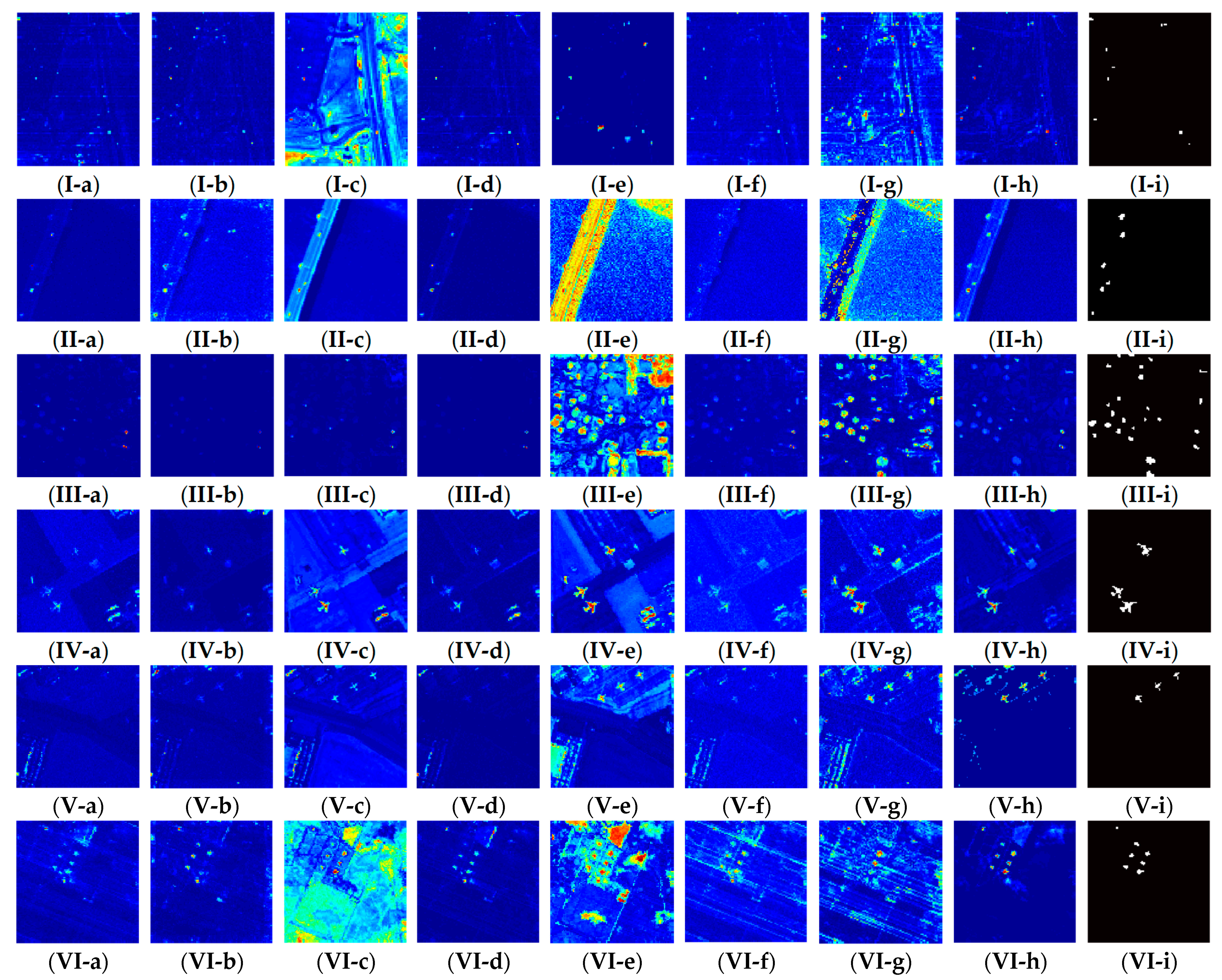
4.5. Detection Performance

The detection maps and three evaluation results mentioned in Section 4.1.2 jointly verify the detection performance. The detection maps over the compared methods on experimental datasets are visualized in Figure 12, and the corresponding AUC values are listed in Table 3. Note that the bold number and shading number in Table 3 stand for the best and second-best results, respectively.
For the HYDICE dataset, the proposed method achieved satisfactory detection results with low false alarm. Obviously, LRASR and KIFD have higher false-alarm rates when compared with other methods. Different from the low detection performance for LRASR, KIFD’s detection performance is superior to other comparative methods, except for the proposed method. The detection results of CRD and PAB-DC are nearly close to those of the proposed method, whereas the detection results of RX, LSMAD and LSDM–MoG are not as good as those of the proposed method, due to, to a large extent, the existence of false alarms and missed inspections.
Figure 12II exhibits the detection maps over comparative methods on the Pavia dataset. It can be seen that the anomalies are completely detected, and the corresponding AUC value (i.e., 0.9951) is best relative to other methods. Although the anomalies are also detected comprehensively for CRD and LRASR, the corresponding AUC values still lower the proposed method, owing to interference of the stronger false alarm. Note that RX and LSMAD show powerful capability in background suppression, whereas the effect of locating anomalies (i.e., 0.9887 and 0.9842) is slightly worse than that of the proposed method. Additionally, the detection performance for PAB-DC, LSDM–MoG and KIFD is poor, as the anomalies are submerged into the background.
For the Los Angeles dataset, the proposed method has the highest AUC value (i.e., 0.9968) compared with other methods. Though RX, CRD, LRASR and LSMAD demonstrate dramatic superiority with respect to background suppression, the ability to locate anomalies is slightly insufficient, especially for LRASR. LSDM–MoG and KIFD can excavate the anomalies as much as possible, with a slightly larger false alarm than the proposed method. In addition, there is a very low AUC value (i.e., 0.8757) and high false alarm for PAB-DC among all comparative methods.
In terms of the San Diego-I dataset, the proposed method is evidently superior to other comparative methods in regard to the AUC value, except for KIFD, which is slightly lower than the proposed method, whereas the false alarm of KIFD is much higher than that of the proposed method. Although the anomalies can be completely located in RX, LRASR, PAB-DC and LSDM–MoG, the higher false alarm is harmful to the detection performance. Note that the ability to perform background suppression for CRD and LSMAD is better than for other compared methods, while the effect of detecting anomalies is poor.
With respect to the San Diego-II dataset, the proposed method can detect anomalies comprehensively and obtain a superior performance in regard to the AUC value (i.e., 0.9986) relative to other methods. Compared with the proposed method, RX, CRD and LSMAD have a lower false-alarm rate, while the detection effect of anomalies is not ideal. LRASR, PAB-DC and KIFD achieve competitive detection results in regard to AUC values. Even worse, the anomalies fail to be detected comprehensively, and the effect of background suppression is also poor for LSDM–MoG.
For the Texas Coast dataset, the proposed method achieved optimal results for the AUC value, which is 0.9969. For RX, CRD and LSMAD, most anomalies were detected with a slight low false alarm. Conversely, LRASR, PAB-DC, LSDM–MoG and KIFD retained a very high false alarm.
Furthermore, to analyze the detection performance of the comparative methods, ROC curves are plotted in Figure 13. For better visualization, the ROC curves are shown in a logarithmic-scale manner. By observing Figure 13, we can see that the curve of the proposed method is higher than other methods on all experimental datasets, meaning that the effect of locating anomalies outperforms other methods.
Additionally, the separability range between anomaly and background is executed on experimental datasets, as illustrated in Figure 14. By observing Figure 14, we can find that the distance between the lower bound of the red box and the upper bound of the green box corresponding to the proposed method is larger than that of other methods, thus indicating that the separability effect of the proposed method is superior to that of the other methods. Based on the above analysis, the proposed method can be regarded as a competitive anomaly detector for HSIs.

5. Discussion

In this section, we analyze the experiment effect of the proposed method from two aspects (i.e., strength and limitation) and make a parallel comparison with the state-of-the-art models based on deep learning. As described in Section 4, a comprehensive comparison consisting of both qualitative and quantitative perspectives was executed on experimental datasets with four classical and three state-of-the-art methods. Concretely, we used two qualitative metrics (i.e., ROC curve and separability range of the background–anomaly) to evaluate the performance of the proposed method. By observing the ROC curves illustrated in Figure 13, we can easily find that the ROC curves of the proposed method are higher than other methods on overall experimental datasets, especially for HYDICE, Los Angeles, San Diego-II and the Texas Coast. For the separability range of background–anomaly, we can also see that the distance between background and anomaly is larger than other methods, thus indicating that the discrimination of the background and anomaly is greater than that of other methods. From the perspective of quantitative analysis, the AUC value is adopted as the indicator to judge the performance of the proposed method. The detailed AUC values of different experimental datasets are shown in Table 3. Through Table 3, we can find that the average AUC value on overall datasets is up to 0.9965, which is higher than the second best comparison method (i.e., 0.9813 for LSMAD). This means that the proposed method outperforms other methods to a large extent. Additionally, the effectiveness of each component proposed in this paper is also validated in Section 4.
According to the above analysis, the detection results of the proposed method are evidently competitive relative to the comparative methods. However, due to the high complexity of the proposed method, the computation complexity of proposed method is clearly much higher than the most comparative methods. For a clear illustration, the computation time of different methods is given in Table 4. Here, the bold number and shading number refer to the best and second-best results, respectively. By observing Table 4, it can be seen that the computing time of the proposed method is slightly more than that of PAB-DC, while the computing time of the other methods, excluding PAB-DC, are far less than that of the proposed method, especially the RX detector. Clearly, the low real-time performance will restrict the application of the proposed method in the engineering field. Hence, it will be a good choice to lower the complexity of our method in the future.
Additionally, considering the fact that our method is a combination of an autoencoder and generative adversarial network, in essence, it is a deep learning-based method. Therefore, it is necessary to make a parallel comparison with the state-of-the-art models based on deep learning. In terms of the existing deep-learning-based methods, the deep feature or reconstruction information of the observed data is generally adopted to measure the anomaly, which has a limited performance due to the fact that only the single-stage information is employed in these methods. To further improve the detection performance, our method fully uses the two-stage complementary information. Clearly, the two-stage complementary information is obviously superior to the single-stage information, as shown in Table 2, meaning that the proposed method is competitive to existing deep-learning-based methods.

6. Conclusions

In this paper, we proposed a novel dual dictionaries construction method via two-stage complementary decision for HAD. To alleviate the influence of the pixels with similar characteristics to the testing anomalous pixels, we proposed an adaptive inner window–based saliency detection to detect anomalies. With this situation, a coarse binary map was obtained. In order to acquire a fine binary map, a background estimation network, which is trained with the background pixels obtained under the guidance of coarse binary map, was designed. Finally, the coarse and fine binary maps jointly worked together to select representative atoms for background and potential anomaly dictionaries, with the help of superpixels. To validate the effect of the proposed method, extensive experiments on five datasets consisting of six HSIs were conducted. The experiment results show that the average AUC value (i.e., 0.9965) of the proposed method outperforms that of other methods, while the average computing time (i.e., 364.54 s) of the former is lower than that of the latter. In summary, this strategy of two-stage complementary decision paves a new way for studying HAD.
To alleviate the poor real-time performance of the proposed method, in the future, we will attempt to replace the two stages of the proposed method with a simpler model, which ensures that the complexity of model is far less than that of the proposed method. Once the model is obtained, we will further deploy it for a mobile device.

Author Contributions

S.L., H.W. and M.Z. provided the ideas; S.L., X.C., L.W. and M.X. implemented this algorithm; S.L. wrote this paper; H.W. and M.Z. revised this paper. All authors have read and agreed to the published version of the manuscript.

Funding

This research was funded by the National Natural Science Foundation of China (No. 12003018), Fundamental Research Funds for the Central Universities (No. XJS191305) and China Postdoctoral Science Foundation (No. 2018M633471).

Data Availability Statement

The dataset used in this paper can be download from http://xudongkang.weebly.com/ (accessed on 5 March 2022).

Acknowledgments

We thank the authors who provided experimental datasets and compared methods. Also, our experiments are supported by High-performance Computing Platform of XiDian University.

Conflicts of Interest

The authors declare no conflict of interest.

References

  1. Lu, B.; Dao, P.D.; Liu, J.; He, Y.; Shang, J. Recent Advances of Hyperspectral Imaging Technology and Applications in Agriculture. Remote Sens. 2020, 12, 2659. [Google Scholar] [CrossRef]
  2. Zou, L.; Zhang, Z.; Du, H.; Lei, M.; Xue, Y.; Wang, Z.J. Da-Imrn: Dual-Attention-Guided Interactive Multi-Scale Residual Network for Hyperspectral Image Classification. Remote Sens. 2022, 14, 530. [Google Scholar] [CrossRef]
  3. Shah, C.; Du, Q.; Xu, Y. Enhanced Tabnet: Attentive Interpretable Tabular Learning for Hyperspectral Image Classification. Remote Sens. 2022, 14, 716. [Google Scholar] [CrossRef]
  4. Su, Y.; Li, J.; Plaza, A.; Marinoni, A.; Gamba, P.; Chakravortty, S. Daen: Deep Autoencoder Networks for Hyperspectral Unmixing. IEEE Trans. Geosci. Remote Sens. 2019, 57, 4309–4321. [Google Scholar] [CrossRef]
  5. Dong, L.; Yuan, Y. Sparse Constrained Low Tensor Rank Representation Framework for Hyperspectral Unmixing. Remote Sens. 2021, 13, 1473. [Google Scholar] [CrossRef]
  6. Liu, Y.; Li, X.; Hua, Z.; Zhao, L. Ebarec-Bs: Effective Band Attention Reconstruction Network for Hyperspectral Imagery Band Selection. Remote Sens. 2021, 13, 3602. [Google Scholar] [CrossRef]
  7. Wang, Q.; Zhang, F.; Li, X. Optimal Clustering Framework for Hyperspectral Band Selection. IEEE Trans. Geosci. Remote Sens. 2018, 56, 5910–5922. [Google Scholar] [CrossRef] [Green Version]
  8. Yu, S.; Li, X.; Chen, S.; Zhao, L. Exploring the Intrinsic Probability Distribution for Hyperspectral Anomaly Detection. Remote Sens. 2022, 14, 441. [Google Scholar] [CrossRef]
  9. Zhang, L.; Ma, J.; Cheng, B.; Lin, F. Fractional Fourier Transform-Based Tensor Rx for Hyperspectral Anomaly Detection. Remote Sens. 2022, 14, 797. [Google Scholar] [CrossRef]
  10. Macfarlane, F.; Murray, P.; Marshall, S.; White, H. Investigating the Effects of a Combined Spatial and Spectral Dimensionality Reduction Approach for Aerial Hyperspectral Target Detection Applications. Remote Sens. 2021, 13, 1647. [Google Scholar] [CrossRef]
  11. Zhu, D.; Du, B.; Zhang, L. Target Dictionary Construction-Based Sparse Representation Hyperspectral Target Detection Methods. IEEE J. Sel. Top. Appl. Earth Obs. Remote Sens. 2019, 12, 1254–1264. [Google Scholar] [CrossRef]
  12. Yang, Y.; Zhang, J.; Song, S.; Zhang, C.; Liu, D. Low-Rank and Sparse Matrix Decomposition with Orthogonal Subspace Projection-Based Background Suppression for Hyperspectral Anomaly Detection. IEEE Geosci. Remote Sens. Lett. 2019, 17, 1378–1382. [Google Scholar] [CrossRef]
  13. Bai, Z.; Liu, Z.; Li, G.; Ye, L.; Wang, Y. Circular Complement Network for Rgb-D Salient Object Detection. Neurocomputing 2021, 451, 95–106. [Google Scholar] [CrossRef]
  14. Qian, X.; Cheng, X.; Cheng, G.; Yao, X.; Jiang, L. Two-Stream Encoder Gan with Progressive Training for Co-Saliency Detection. IEEE Signal Process. Lett. 2021, 28, 180–184. [Google Scholar] [CrossRef]
  15. Liu, W.; Feng, X.; Wang, S.; Hu, B.; Gan, Y.; Zhang, X.; Lei, T. Random Selection-Based Adaptive Saliency-Weighted Rxd Anomaly Detection for Hyperspectral Imagery. Int. J. Remote Sens. 2018, 39, 2139–2158. [Google Scholar] [CrossRef]
  16. Hou, Z.; Li, W.; Tao, R.; Ma, P.; Shi, W. Collaborative Representation with Background Purification and Saliency Weight for Hyperspectral Anomaly Detection. Sci. China Inf. Sci. 2022, 65, 112305. [Google Scholar] [CrossRef]
  17. Goferman, S.; Zelnik-Manor, L.; Tal, A. Context-Aware Saliency Detection. IEEE Trans. Pattern Anal. Mach. Intell. 2012, 34, 1915–1926. [Google Scholar] [CrossRef] [Green Version]
  18. Yu, J.; Rui, Y.; Tang, Y.Y.; Tao, D. High-Order Distance-Based Multiview Stochastic Learning in Image Classification. IEEE Trans. Cybern. 2014, 44, 2431–2442. [Google Scholar] [CrossRef] [PubMed]
  19. Huyan, N.; Zhang, X.; Zhou, H.; Jiao, L. Hyperspectral Anomaly Detection via Background and Potential Anomaly Dictionaries Construction. IEEE Trans. Geosci. Remote Sens. 2019, 57, 2263–2276. [Google Scholar] [CrossRef] [Green Version]
  20. Reed, I.S.; Yu, X. Adaptive Multiple-Band Cfar Detection of an Optical Pattern with Unknown Spectral Distribution. IEEE Trans. Acoust. Speech Signal Process. 1990, 38, 1760–1770. [Google Scholar] [CrossRef]
  21. Molero, J.M.; Garzon, E.M.; Garcia, I.; Plaza, A. Analysis and Optimizations of Global and Local Versions of the Rx Algorithm for Anomaly Detection in Hyperspectral Data. IEEE J. Sel. Top. Appl. Earth Obs. Remote Sens. 2013, 6, 801–814. [Google Scholar] [CrossRef]
  22. Guo, Q.; Zhang, B.; Ran, Q.; Gao, L.; Li, J.; Plaza, A. Weighted-Rxd and Linear Filter-Based Rxd: Improving Background Statistics Estimation for Anomaly Detection in Hyperspectral Imagery. IEEE J. Sel. Top. Appl. Earth Obs. Remote Sens. 2014, 7, 2351–2366. [Google Scholar] [CrossRef]
  23. Heesung, K.; Nasrabadi, N.M. Kernel Rx-Algorithm: A Nonlinear Anomaly Detector for Hyperspectral Imagery. IEEE Trans. Geosci. Remote Sens. 2005, 43, 388–397. [Google Scholar] [CrossRef]
  24. Tao, R.; Zhao, X.; Li, W.; Li, H.-C.; Du, Q. Hyperspectral Anomaly Detection by Fractional Fourier Entropy. IEEE J. Sel. Top. Appl. Earth Obs. Remote Sens. 2019, 12, 4920–4929. [Google Scholar] [CrossRef]
  25. Li, W.; Du, Q. Collaborative Representation for Hyperspectral Anomaly Detection. IEEE Trans. Geosci. Remote Sens. 2015, 53, 1463–1474. [Google Scholar] [CrossRef]
  26. Li, J.; Zhang, H.; Zhang, L.; Ma, L. Hyperspectral Anomaly Detection by the Use of Background Joint Sparse Representation. IEEE J. Sel. Top. Appl. Earth Obs. Remote Sens. 2015, 8, 2523–2533. [Google Scholar] [CrossRef]
  27. Zhang, Y.; Du, B.; Zhang, L.; Wang, S. A Low-Rank and Sparse Matrix Decomposition-Based Mahalanobis Distance Method for Hyperspectral Anomaly Detection. IEEE Trans. Geosci. Remote Sens. 2016, 54, 1376–1389. [Google Scholar] [CrossRef]
  28. Xu, Y.; Wu, Z.; Li, J.; Plaza, A.; Wei, Z. Anomaly Detection in Hyperspectral Images Based on Low-Rank and Sparse Representation. IEEE Trans. Geosci. Remote Sens. 2016, 54, 1990–2000. [Google Scholar] [CrossRef]
  29. Li, L.; Li, W.; Du, Q.; Tao, R. Low-Rank and Sparse Decomposition with Mixture of Gaussian for Hyperspectral Anomaly Detection. IEEE Trans. Cybern. 2020, 51, 4363–4372. [Google Scholar] [CrossRef] [PubMed]
  30. Cheng, T.; Wang, B. Graph and Total Variation Regularized Low-Rank Representation for Hyperspectral Anomaly Detection. IEEE Trans. Geosci. Remote Sens. 2019, 58, 391–406. [Google Scholar] [CrossRef]
  31. LeCun, Y.; Bengio, Y.; Hinton, G. Deep Learning. Nature 2015, 521, 436–444. [Google Scholar] [CrossRef] [PubMed]
  32. Qian, X.; Lin, S.; Cheng, G.; Yao, X.; Ren, H.; Wang, W. Object Detection in Remote Sensing Images Based on Improved Bounding Box Regression and Multi-Level Features Fusion. Remote Sens. 2020, 12, 143. [Google Scholar] [CrossRef] [Green Version]
  33. Zhou, K.; Zhang, M.; Wang, H.; Tan, J. Ship Detection in Sar Images Based on Multi-Scale Feature Extraction and Adaptive Feature Fusion. Remote Sens. 2022, 14, 755. [Google Scholar] [CrossRef]
  34. Li, W.; Wu, G.; Du, Q. Transferred Deep Learning for Anomaly Detection in Hyperspectral Imagery. IEEE Geosci. Remote Sens. Lett. 2017, 14, 597–601. [Google Scholar] [CrossRef]
  35. Zhang, L.; Cheng, B. Transferred Cnn Based on Tensor for Hyperspectral Anomaly Detection. IEEE Geosci. Remote Sens. Lett. 2020, 17, 2115–2119. [Google Scholar] [CrossRef]
  36. Wang, S.; Wang, X.; Zhang, L.; Zhong, Y. Auto-Ad: Autonomous Hyperspectral Anomaly Detection Network Based on Fully Convolutional Autoencoder. IEEE Trans. Geosci. Remote Sens. 2022, 60, 5503314. [Google Scholar] [CrossRef]
  37. Zhao, C.; Zhang, L. Spectral-Spatial Stacked Autoencoders Based on Low-Rank and Sparse Matrix Decomposition for Hyperspectral Anomaly Detection. Infrared Phys. Technol. 2018, 92, 166–176. [Google Scholar] [CrossRef]
  38. Xie, W.; Liu, B.; Li, Y.; Lei, J.; Du, Q. Autoencoder and Adversarial-Learning-Based Semisupervised Background Estimation for Hyperspectral Anomaly Detection. IEEE Trans. Geosci. Remote Sens. 2020, 58, 5416–5427. [Google Scholar] [CrossRef]
  39. Arisoy, S.; Nasrabadi, N.M.; Kayabol, K. Unsupervised Pixel-Wise Hyperspectral Anomaly Detection via Autoencoding Adversarial Networks. IEEE Geosci. Remote Sens. Lett. 2021, 19, 5502905. [Google Scholar] [CrossRef]
  40. Jiang, T.; Li, Y.; Xie, W.; Du, Q. Discriminative Reconstruction Constrained Generative Adversarial Network for Hyperspectral Anomaly Detection. IEEE Trans. Geosci. Remote Sens. 2020, 58, 4666–4679. [Google Scholar] [CrossRef]
  41. Jiang, K.; Xie, W.; Li, Y.; Lei, J.; He, G.; Du, Q. Semisupervised Spectral Learning with Generative Adversarial Network for Hyperspectral Anomaly Detection. IEEE Trans. Geosci. Remote Sens. 2020, 58, 5224–5236. [Google Scholar] [CrossRef]
  42. Xie, W.; Zhang, X.; Li, Y.; Lei, J.; Li, J.; Du, Q. Weakly Supervised Low-Rank Representation for Hyperspectral Anomaly Detection. IEEE Trans. Cybern. 2021, 51, 3889–3900. [Google Scholar] [CrossRef] [PubMed]
  43. Yang, Y.; Zhang, J.; Liu, D.; Wu, X. Low-Rank and Sparse Matrix Decomposition with Background Position Estimation for Hyperspectral Anomaly Detection. Infrared Phys. Technol. 2019, 96, 213–227. [Google Scholar] [CrossRef]
  44. Ren, X.; Malik, J. Learning a Classification Model for Segmentation. In Proceedings of the IEEE International Conference on Computer Vision, Nice, France, 13–16 October 2003; pp. 13–16. [Google Scholar]
  45. Achanta, R.; Shaji, A.; Smith, K.; Lucchi, A.; Fua, P.; Süsstrunk, S. Slic Superpixels Compared to State-of-the-Art Superpixel Methods. IEEE Trans. Pattern Anal. Mach. Intell. 2012, 34, 2274–2282. [Google Scholar] [CrossRef] [Green Version]
  46. Zhao, C.; Li, C.; Feng, S.; Su, N.; Li, W. A Spectral–Spatial Anomaly Target Detection Method Based on Fractional Fourier Transform and Saliency Weighted Collaborative Representation for Hyperspectral Images. IEEE J. Sel. Top. Appl. Earth Obs. Remote Sens. 2020, 13, 5982–5997. [Google Scholar] [CrossRef]
  47. Otsu, N. A Threshold Selection Method from Gray-Level Histograms. IEEE Trans. Syst. Man Cybern. Syst. 1979, 9, 62–66. [Google Scholar] [CrossRef] [Green Version]
  48. LeCun, Y.; Bottou, L.; Bengio, Y.; Haffner, P. Gradient-Based Learning Applied to Document Recognition. Proc. IEEE 1998, 86, 2278–2324. [Google Scholar] [CrossRef] [Green Version]
  49. Eckstein, J.; Bertsekas, D.P. On the Douglas—Rachford Splitting Method and the Proximal Point Algorithm for Maximal Monotone Operators. Math. Program. 1992, 55, 293–318. [Google Scholar] [CrossRef] [Green Version]
  50. Cai, J.-F.; Candès, E.J.; Shen, Z. A Singular Value Thresholding Algorithm for Matrix Completion. SIAM J. Optim. 2010, 20, 1956–1982. [Google Scholar] [CrossRef]
  51. Lin, Z.; Chen, M.; Ma, Y. The Augmented Lagrange Multiplier Method for Exact Recovery of Corrupted Low-Rank Matrices. arXiv 2010, arXiv:1009.5055. [Google Scholar]
  52. Li, S.; Zhang, K.; Duan, P.; Kang, X. Hyperspectral Anomaly Detection with Kernel Isolation Forest. IEEE Trans. Geosci. Remote Sens. 2019, 58, 319–329. [Google Scholar] [CrossRef]
  53. Kang, X.; Zhang, X.; Li, S.; Li, K.; Li, J.; Benediktsson, J.A. Hyperspectral Anomaly Detection with Attribute and Edge-Preserving Filters. IEEE Trans. Geosci. Remote Sens. 2017, 55, 5600–5611. [Google Scholar] [CrossRef]
  54. Bradley, A.P. The Use of the Area under the Roc Curve in the Evaluation of Machine Learning Algorithms. Pattern Recognit. 1997, 30, 1145–1159. [Google Scholar] [CrossRef] [Green Version]
  55. Huang, J.; Ling, C.X. Using Auc and Accuracy in Evaluating Learning Algorithms. IEEE Trans. Knowl. Data Eng. 2005, 17, 299–310. [Google Scholar] [CrossRef] [Green Version]
  56. Manolakis, D.; Shaw, G. Detection Algorithms for Hyperspectral Imaging Applications. IEEE Signal Process. Mag. 2002, 19, 29–43. [Google Scholar] [CrossRef]
  57. Srivastava, N.; Hinton, G.; Krizhevsky, A.; Sutskever, I.; Salakhutdinov, R. Dropout: A Simple Way to Prevent Neural Networks from Overfitting. J. Mach. Learn. Res. 2014, 15, 1929–1958. [Google Scholar]
  58. Kingma, D.P.; Ba, J. Adam: A Method for Stochastic Optimization. arXiv 2014, arXiv:1412.6980. [Google Scholar]
  59. Jin, Q.; Ma, Y.; Mei, X.; Ma, J. Tanet: An Unsupervised Two-Stream Autoencoder Network for Hyperspectral Unmixing. IEEE Trans. Geosci. Remote Sens. 2021, 60, 5506215. [Google Scholar] [CrossRef]
Figure 1. Visualization of chosen atoms in background and potential anomaly dictionaries for PAB-DC and the proposed method on the Los Angeles dataset. Here, green dots indicate chosen atoms in background and potential anomaly dictionaries, and the red areas represent the corresponding anomalies in the reference map. Note: (I,II) stand for the PAB-DC and the proposed method, respectively; (a,b) separately refer to the background dictionary and potential anomaly dictionary.
Remotesensing 14 01784 g001
Figure 2. Schematic of the proposed method. Note: “ B 1 b m p ” in “Coarse Background–Anomaly Separation” and “LRSR based on DDC–TSCD” is the same. In addition, the “ x b a c 1 , , x b a c S b ” in “” and “” is the same.
Remotesensing 14 01784 g002
Figure 3. Illustration of dual windows: (a) dual rectangular windows; (b) adaptive inner window and rectangular outer window.
Remotesensing 14 01784 g003
Figure 4. Comparison of the original and reconstructed spectral information on San Diego-II. Here, “A1_0” represents the anomalous pixel “A1” in original HSI. “A1_1” indicates the anomalous pixel “A1” in the reconstructed HSI. Similarly, “B1_0” and “B1_1” signify the background pixel “B1” in original HSI and reconstructed HSI, respectively.
Remotesensing 14 01784 g004
Figure 5. An example to illustrate the construction process of background and potential anomaly dictionaries on the Texas Coast. Here, (ag) separately indicate the coarse binary map, fine binary map, the sum of two binary maps, the product of two binary maps, superpixel segmentation result, background dictionary index map and potential anomaly dictionary index map. The symbols and are addition operation and multiplication operation pixel by pixel, respectively. Note that the elements whose values are “1” in (f,g) are employed to act as the index to select the atoms for background and potential anomaly dictionaries.
Remotesensing 14 01784 g005
Figure 6. Visualization of the experimental datasets: (a) color composites and (b) reference map; (I) HYDICE, (II) Pavia, (III) Los Angeles, (IV) San Diego-I, (V) San Diego-II and (VI) Texas Coast.
Remotesensing 14 01784 g006
Figure 7. Effect of parameter K over AUC values on experimental datasets.
Remotesensing 14 01784 g007
Figure 8. Effect of parameter R over AUC values on experimental datasets.
Remotesensing 14 01784 g008
Figure 9. Effect of parameter λ and β on AUC values for proposed method on (a) Pavia and (b) Los Angeles.
Remotesensing 14 01784 g009
Figure 10. Histogram of the comparison results between the adaptive inner window–based method and dual rectangular windows–based method on experimental datasets. Here, “3”, “5”, “7”, “9” and “11” represent the size of inner window in dual rectangular windows, “AW” denotes the adaptive inner window.
Remotesensing 14 01784 g010
Figure 11. Visualization of detection map for the Los Angeles dataset on (a) dual dictionaries construction with only coarse binary map. (b) Dual dictionaries construction with only fine binary map. (c) Dual dictionaries construction with two-stage complementary decision.
Remotesensing 14 01784 g011
Figure 12. Detection maps of different methods: (I) HYDICE, (II) Pavia, (III) Los Angeles, (IV) San Diego-I, (V) San Diego-II and (VI) Texas Coast. (a) RX, (b) CRD, (c) LRASR, (d) LSMAD, (e) PAB-DC, (f) LSDM–MoG, (g) KIFD, (h) proposed method and (i) ground truth.
Remotesensing 14 01784 g012
Figure 13. ROC curves for different methods on (a) HYDICE, (b) Pavia, (c) Los Angeles, (d) San Diego-I, (e) San Diego-II and (f) Texas Coast.
Remotesensing 14 01784 g013
Figure 14. Anomaly–background separability maps of different methods on (a) HYDICE, (b) Pavia, (c) Los Angeles, (d) San Diego-I, (e) San Diego-II and (f) Texas Coast. Here, letters “a–h” stand for RX, CRD, LRASR, LSMAD, PAB-DC, LSDM–MoG, KIFD and proposed method, respectively.
Remotesensing 14 01784 g014
Table 1. Optimal parameters settings for experimental datasets.
ParametersHYDICEPaviaLos AngelesSan Diego-ISan Diego-ITexas Coast
K400400400400400400
R777777
Λ10.010.01111
Β0.010.0010.0010.010.10.1
Table 2. Component analysis results for experimental datasets.
HYDICEPaviaLos AngelesSan Diego-ISan Diego-IITexas Coast
Coarse0.97000.96220.98650.98900.99400.9955
Fine0.98620.97280.99230.99160.99730.9951
Complementary0.99910.99510.99680.99230.99860.9969
Table 3. AUC values on different methods over five datasets.
DatasetRXCRDLRASRLSMADPAB-DCLSDM–MoGKIFDDDC–TSCD
HYDICE0.98570.99510.84020.98610.99550.97920.99660.9991
Pavia0.98870.96500.98890.98420.88580.94820.85890.9951
Los Angeles0.98870.97940.87480.98140.87570.97450.97660.9968
San Diego-I0.94030.94120.89500.97010.97800.93390.99140.9923
San Diego-II0.91110.97910.98530.97320.99410.93200.99220.9986
Texas Coast0.99070.97960.76560.99280.97470.99130.93540.9969
Average0.96750.97320.89160.98130.95060.95990.95850.9965
Table 4. Computing time (in seconds) on different methods over five datasets.
DatasetRXCRDLRASRLSMADPAB-DCLSDM–MoGKIFDDDC–TSCD
HYDICE0.232.6229.848.25257.156.6146.42265.32
Pavia0.299.4839.1613.93352.128.5756.37364.18
Los Angeles0.385.9042.1212.47358.5210.6454.09376.80
San Diego-I0.3310.1541.6011.61362.689.2166.59380.19
San Diego-II0.5215.0653.8917.67410.2316.0968.31430.22
Texas Coast0.367.2444.2512.76354.4311.8463.61370.51
Average0.358.4141.8112.78349.1910.4959.23364.54
Publisher’s Note: MDPI stays neutral with regard to jurisdictional claims in published maps and institutional affiliations.

