Article

A Novel Method for Fast Kernel Minimum Noise Fraction Transformation in Hyperspectral Image Dimensionality Reduction

1
Key Laboratory of Space Active Opto-Electronics Technology, Shanghai Institute of Technical Physics, Chinese Academy of Sciences, Shanghai 200083, China
2
University of Chinese Academy of Sciences, Beijing 100049, China
3
Hangzhou Institute for Advanced Study, University of Chinese Academy of Sciences, Hangzhou 310024, China
4
Research Center for Intelligent Sensing Systems, Zhejiang Laboratory, Hangzhou 311100, China
*
Author to whom correspondence should be addressed.
Remote Sens. 2022, 14(7), 1737; https://doi.org/10.3390/rs14071737
Submission received: 3 March 2022 / Revised: 30 March 2022 / Accepted: 2 April 2022 / Published: 4 April 2022

Abstract

:
Feature extraction, aiming to simplify and optimize data features, is a typical hyperspectral image dimensionality reduction technique. As a kernel-based method, kernel minimum noise fraction (KMNF) transformation is excellent at handling the nonlinear features within HSIs. It adopts the kernel function to ensure data linear separability by transforming the original data to a higher feature space, following which a linear analysis can be performed in this space. However, KMNF transformation has the problem of high computational complexity and low execution efficiency. It is not suitable for the processing of large-scale datasets. In terms of this problem, this paper proposes a graphics processing unit (GPU) and Nyström method-based algorithm for Fast KMNF transformation (GNKMNF). First, the Nyström method estimates the eigenvector of the entire kernel matrix in KMNF transformation by the decomposition and extrapolation of the sub-kernel matrix to reduce the computational complexity. Then, the sample size in the Nyström method is determined utilizing a proportional gradient selection strategy. Finally, GPU parallel computing is employed to further improve the execution efficiency. Experimental results show that compared with KMNF transformation, improvements of up to 1.94% and 2.04% are achieved by GNKMNF in overall classification accuracy and Kappa, respectively. Moreover, with a data size of 64 × 64 × 250, the execution efficiency of GNKMNF speeds up by about 80×. The outcome demonstrates the significant performance of GNKMNF in feature extraction and execution efficiency.

1. Introduction

Hyperspectral remote sensing, which provides numerous information sources for monitoring human activities and systems of the Earth, has been widely used in various fields, such as crop analysis, mineral identification, geological research, and environmental mapping [1,2,3]. However, because of the enormous spectral bands contained in hyperspectral images (HSIs), their analysis has become a challenging and computationally expensive task [1,4]. Therefore, it is necessary to discard redundant information in HSIs without losing their desirable features [5]. As an effective tool to solve this problem, dimensionality reduction (DR) has become a critical step in HSI processing tasks [6]. It can bring benefits by: (1) improving the statistical ill-conditioning problem by discarding redundant features; (2) reducing computational complexity and storage pressure; and (3) avoiding the Hughes phenomenon (that is, when a fixed training sample size is given, the classifier performance first improves as the dimensionality increases but then degrades when the dimensionality is higher than the optimal value) existing in an HSI classification task [5,6].
A variety of DR methods has been proposed over the years. Presently, they are separated into two main categories: feature extraction and band selection. Band selection methods are designed to select a subset of hyperspectral spectral features to remove spectral redundancy, while retaining the important information of the entire image [7]. The hyperspectral band selection methods can be divided into six major classes: hybrid-scheme-based methods [8,9,10], embedding learning-based methods [7], searching-based methods [11,12], ranking-based methods [13,14,15], clustering-based methods [16,17,18], and sparsity-based methods [19,20,21]. However, it is difficult to determine the optimal band number and comprehensively assess the performance of band selection [6,7]. Unlike band selection, feature extraction transforms the original data into the optimized space by mathematical manipulation [22]. Many methods have been presented for feature extraction. Traditional feature extractions can be categorized as linear and nonlinear methods. Principal component analysis (PCA) [23], minimum noise fraction (MNF) transformation [24], linear discriminant analysis (LDA) [25], non-negative matrix underapproximation (NMU) [26], and non-negative matrix factorization (NMF) [27] are commonly used linear feature extraction methods. The nonlinear methods can be categorized into kernel-based methods [28,29], manifold-learning-based methods [30,31,32], and graph-theory-based methods [33]. By imposing the nonnegative constraint, NMF retains the non-negativity of HSIs in the lower feature space. Introducing a recursive procedure to NMF, NMU has the advantage of identifying features sequentially. However, because they ignore the inherent geometric structure information of the original data, it is difficult for both NMF and NMU to produce desired results when the data are nonlinear [34]. LDA is a supervised feature extraction method. It projects the initial data to the lower space where the distances between different class centers are maximized [25]. In contrast, this supervised method requires prior knowledge of categories and is unsuitable for complex scenes. Utilizing information content as an assessment index, PCA sorts the components by descending order [23]; however, its performance relies heavily on the noise characteristics of the original data. It cannot guarantee that the components are ordered following the image quality when the noise is distributed unevenly in each band [24], whereas MNF solves this problem and produces new components arranged by image quality, no matter how the noise is distributed [24].
Because of factors such as the interaction of ground objects within one pixel, atmospheric absorption, and scattering, HSIs have inherent nonlinear characteristics [35]. It is difficult for the aforementioned methods to deal with the nonlinear features effectively and efficiently within the HSIs. Recently, deep learning architectures and kernel functions have achieved remarkable success in dealing with the nonlinear features. Deep learning methods employ a hierarchical framework to extract high-dimensional features [36]. A convolutional neural network (CNN), which contains multiple hidden layers, can extract features without manual annotation of attributes [37,38]. Chen et al. [39] extracted the deep spatial-spectral features of HSIs using CNN, and achieved high classification performance. Although CNN is excellent in feature extraction, the high-dimensional data of HSIs place a heavy load on the computational process. In terms of this issue, Feng et al. [40] combined the multibranch CNN with attention mechanisms (AMs) to obtain features in an adaptive region search. Mou et al. [41] employed a squeeze-and-excitation network (SENet) to suppress redundancy and strengthen the vital bands. Adopting a nonlocal neural network (NLNN), Xue et al. [42] developed Gaussian-like distribution weights of feature maps to generate the second-order features of HSIs for classification. In addition, Li et al. [43] exploited the manifold-based maximization margin discriminant network (M3DNet) to improve the feature extraction ability of deep learning models. In recent years, various feature extraction methods were developed based on different deep learning frameworks. However, finding the favorable number and size of hidden units for specific problems is a major problem with deep learning frameworks [36]. The kernel functions ensure data linear separability by transforming the original data to the higher feature space, following which a linear analysis can be performed in this space [44]. As a kernel-based method, kernel MNF (KMNF) [28] transformation adopts kernel functions [45] to make up for the weakness of MNF in modelling the nonlinear features within the HSIs. While KMNF is a valuable feature extraction method for HSIs, KMNF transformation presents the problem of high computational complexity and low execution efficiency. It is not suitable for the processing of large-scale datasets. In terms of this problem, this paper proposes a novel method for fast KMNF transformation (GNKMNF) based on the Nyström method and graphics processing unit (GPU) parallel computing. The contributions of this paper can be summarized as follows:
(1) In this paper, the performance of different feature extraction methods (including PCA, MNF, kernel PCA (KPCA), factor analysis (FA), LDA, local preserving projections (LPP), and KMNF) are evaluated in the Indian Pines, Salinas, and Xiong’an datasets. The experimental results show the generalization and effectiveness of KMNF transformation in feature extraction, which provides a reference for further research in feature extraction.
(2) In terms of high computational complexity and low execution efficiency of KMNF transformation, the Nyström method is introduced to estimate the eigenvector of the entire kernel matrix by the decomposition and extrapolation of the sub-kernel matrix. The experimental results demonstrate that the Nyström method-based KMNF (NKMNF) transformation has lower computational complexity and achieves satisfactory results in classification. The proposed framework can be developed as a general model for the real-time implementation of other algorithms.
(3) The sample size of the sub-kernel matrix in NKMNF transformation is an essential factor that affects the result. This paper determines the sample size of the sub-kernel matrix by utilizing a proportional gradient selection strategy. Experimental results suggest that when the proportion of sub-kernel matrix in the entire kernel matrix is 20%, the improvement of the NKMNF transformation in overall classification accuracy and Kappa is up to 1.94% and 2.04% compared with the KMNF transformation. Moreover, with a data size of 64 × 64 × 250, the execution efficiency of the NKMNF transformation speeds up by about 8x.
(4) In this paper, GPU parallel computing is employed to improve the execution efficiency of NKMNF transformation further. Experimental results show that with a data size of 64 × 64 × 250, the execution efficiency of GNKMNF transformation speeds up by about 10x and 80x compared with NKMNF transformation and KMNF transformation, respectively.
The remainder of this paper is organized as follows. Section 2 introduces the procedures of the Nyström method and GNKMNF transformation. The experiments and results of the proposed method are shown in Section 3. Section 4 describes the analysis of the experimental results, and conclusions are provided in Section 5.

2. Proposed Method

In this section, the KMNF transformation is briefly introduced in Section 2.1, and the proposed method, GNKMNF transformation, is described in Section 2.2.

2.1. KMNF Transformation

Due to atmospheric effects and instrumental noise, HSIs often suffer from disturbing degradations due to various types of noise during the imaging process. The noise includes sparse noise, quantization noise, and thermal noise. Defective instruments can cause sparse noise, such as salt and pepper noise, missing pixels, and other outliers which often exist in HSIs. Quantization and Thermal noise, which are signal-independent, are modeled by Gaussian additive noise [46]. It is considered that noise and signals are independent of each other. For an HSI with b spectral bands and n pixels, the HSI Z with n rows and b columns can be seen as a sum of signal part and noise part [24]:
Z p = Z S p + Z N p ,
where Z p is the pixel vector located at p ; Z S p and Z N p are the signal and noise contained in Z p , respectively. Therefore, the covariance matrix S of image Z can be written as the sum of the signal covariance matrix S S and the noise covariance matrix S N ,
S = S S + S N .
Considering z ¯ i as the average of i th band, the matrix Z m e a n with n rows and b columns can be expressed as follows:
Z m e a n = z ¯ 1 z ¯ 2 z ¯ 1 z ¯ 2 z ¯ b z ¯ b z ¯ 1 z ¯ 2 z ¯ b .
Then, the center matrix X of matrix Z is given by
X = Z + Z m e a n .
The covariance matrix S of image Z could be expressed as
S = X T X / n 1 .
Similarly, considering z ¯ N i as the average of i th band in the noise matrix Z N , the matrix Z N m e a n with n rows and b columns can be expressed as follows:
Z N m e a n = z ¯ N 1 z ¯ N 2 z ¯ N 1 z ¯ N 2 z ¯ N b z ¯ N b z ¯ N 1 z ¯ N 2 z ¯ N b .
Then, the center matrix X N of matrix Z N is given by
X N = Z N + Z N m e a n .
The covariance matrix S of image Z could be expressed as
S N = X N T X N / n 1 .
The noise fraction N F is defined as the ratio of the noise variance matrix of Z N to the image variance matrix of Z . For a linear combination a T X p ,
N F = a T S N a / a T S a = a T X N T X N a / a T X T X a ,  
where a is the eigen matrix of N F .
The KMNF transformation orders the new components according to image quality by minimizing the N F . Minimizing N F is equal to maximizing 1 / N F for mathematics:
1 / N F = a T S a / a T S N a = a T X T X a / a T X N T X N a .
The dual formulation of 1 / N F is obtained by reparametrizing and setting a Z T b [28]:
1 / N F = b T X X T X X T b / b T X X N T X N X T b .
In KMNF transformation, a nonlinear mapping Φ : z Φ z which transforms the original data into higher feature space is introduced to kernelize the 1 / N F [45].
1 / N F = b T Φ X Φ X T Φ X Φ X T b / b T Φ X Φ X N T Φ X N Φ X T b .
1 / N F = b T κ 2 b / b T κ N κ N T b ,
where Φ X is the kernelization matrix of X ; Φ X N is the kernelization matrix of X N ; κ = Φ X Φ X T ; and κ N = Φ X Φ X N T .
The maximized 1 / N F is solved by the maximized Rayleigh entropy, the process can be written as follows:
κ 2 b = λ κ N κ N T b ,  
κ 2 b = λ ( κ N κ N T ) 1 2 ( κ N κ N T ) 1 2 b ,
( κ N κ N T ) 1 2 κ 2 ( κ N κ N T ) 1 2 [ ( κ N κ N T ) 1 2 b = λ ( κ N κ N T ) 1 2 b ] ,
where ( κ N κ N T ) 1 2 b and λ are the eigenvectors and eigenvalues of ( κ N κ N T ) 1 2 κ 2 ( κ N κ N T ) 1 2 , respectively. The matrix b can be obtained from Formula (16).
As mentioned above, X T b transforms to Φ X T b after the nonlinear mapping Φ : z Φ z , the feature extraction result of KMNF transformation Y can be obtained by:
Y = Φ X a = Φ X Φ X T b = κ b .
From the above analysis, it can be seen that noise estimation is a key step in KMNF transformation. The KMNF transformation adopts the spatial neighborhood (3 × 3) feature of HSI to estimate noise Z N [28,47], as described below:
n i , j , k = z i , j , k z ^ i , j , k = z i , j , k ( z i 1 , j 1 , k + 2 z i , j 1 , k z i + 1 , j 1 , k + 2 z i 1 , j , k , + 5 z i , j , k + 2 z i + 1 , j , k z i 1 , j + 1 , k + 2 z i , j + 1 , k z i + 1 , j + 1 , k ) / 9 ,
where z i , j , k is the pixel value located at band k, line i, and column j of the original HSI; z ^ i , j , k is the estimated pixel value; and n i , j , k is the estimated noise of z i , j , k . The procedure for the KMNF transformation is shown in Algorithm 1.
Algorithm 1 KMNF Transformation Procedure
Input: hyperspectral data Z .
Step 1: compute the estimated pixel value z ^ i , j , k .
Step 2: noise estimation: n i , j , k = z i , j , k z ^ i , j , k .
Step 3: the dual transformation, nonlinear mapping, kernelization of 1 / N F is obtained by Formula (12).
Step 4: obtain b by calculating the eigenvectors of ( κ N κ N T ) 1 2 κ 2 ( κ N κ N T ) 1 2 .
Step 5: map all pixels into the transformation result matrix utilizing Formula (17).
Output: the feature extraction result for the KMNF transformation Y .

2.2. The Nyström Method and GPU-Based KMNF Transformation

The Nyström Method was originally used to solve integral equations. Its basic idea is to estimate the decomposition of the entire kernel matrix by calculating the eigenvalues decomposition of the sub-kernel matrix with part of the sample [48].
For a matrix P with N rows and N columns, the affinity block matrix Q of P can be constructed using the formula as follows.
Q = A B B T C ,  
where A represents the left-top matrix with m rows and m   columns from matrix P ; B represents the right-top matrix with m rows and s   columns from matrix P ( m + s = N ,   m s ); C represents a matrix with s rows and s   columns, it can be estimated by
C = B T A 1 B .  
Then, the matrix Q can be expressed as
Q = A B B T B T A 1 B .  
To diagonalize matrix A ,
A = U Λ U T ,  
where U and Λ are the eigenvectors and eigenvalues vector of matrix A , respectively.
The estimated eigenvectors U ˜ of matrix Q can be obtained by
U ˜ = U B T U Λ 1 .  
It must be orthogonal before using because U ˜ is not orthogonal. Defining
K = A + A 1 2 B B T A 1 2 .  
To diagonalize matrix K ,
K = U K Λ K U K T ,  
where U K and Λ K are the eigenvectors and eigenvalues vector of matrix K , respectively.
The estimated eigenvectors V of matrix P can be obtained by
V = A B T A 1 2 U K Λ K 1 2  
From the above analysis, the Nyström method can significantly reduce the computational complexity of obtaining matrix eigenvalues. Nyström method theory is employed in this paper to reduce the computational complexity and improve the execution efficiency of the KMNF transformation. The procedure for the Nyström method-based KMNF (NKMNF) transformation is summarized in Algorithm 2.
Algorithm 2 NKMNF Transformation Procedure
Input: hyperspectral data Z .
Step 1: compute the estimated pixel value z ^ i , j , k .
Step 2: noise estimation: n i , j , k = z i , j , k z ^ i , j , k .
Step 3: the dual transformation, nonlinear mapping, kernelization of 1 / N F is obtained by Formula (12).
Step 4: take ( κ N κ N T ) 1 2 κ 2 ( κ N κ N T ) 1 2 as P , the affinity matrix is obtained by Formula (21).
Step 5: estimate b by calculating the estimated eigenvectors of P by Formula (26).
Step 6: map all pixels into the transformation result matrix utilizing Formula (17).
Output: the feature extraction result for the NKMNF transformation Y .
Parallel computing has received increasing attention because of its tremendous computational power over the years. With multicore processors and multithreading, GPU is more flexible in programming and distinguished in floating-point operation compared with the central processing unit (CPU) and programmable gate array (FPGA) [49]. To execute vector and matrix operations better, NVIDIA computing unified device architecture (CUDA) provides a basic linear algebra subroutines library (called CUBLAS) based on the GPU parallel platform [49]. An analysis of NKMNF shows that there are voluminous vector and matrix multiplication operations in the program. Therefore, this paper further develops the parallel processing of NKMNF based on the GPU CUBLAS.
In this paper, the parallel computing performance of GNKMNF is assessed in the computing hardware composed of an NVIDIA GeForce GTX745 GPU card and an Intel Core i5-4460 CPU at 3.20 GHz with four cores. The NVIDIA GeForce GTX745 hardware specifications are shown in Table 1.

3. Results

The experiments and results of the proposed method are shown in this section. Four experiments were designed to assess the performance of the GNKMNF transformation. Three real HSIs (including the Indian Pines, Salinas, and Xiong’an datasets) with different spatial and spectral resolutions over different scenes used in the experiments are introduced in Section 3.1. The first experiment was designed to evaluate the performance of seven feature extraction methods (including PCA, MNF, KPCA, FA, LDA, LPP, and KMNF) in classification. Taking overall accuracy and Kappa as the assessment criteria, the classification performance of each feature extraction method in terms of the support vector machine (SVM) classifier with a radial basis function (RBF) kernel was evaluated. In this experiment, 25% of samples were randomly chosen for training, the remaining 75% were applied to testing, and ten-fold cross-validation was employed to find the best parameters in SVM. The results are described in Section 3.2. In order to visually show the computational complexity of each feature extraction method, the second experiment tests the runtimes of each method with a data size of 100 × 100 × 250. The test results are shown in Section 3.3. The Nyström method estimates the eigenvector of the entire kernel matrix by the decomposition and extrapolation of the sub-kernel matrix. The sample size of the sub-kernel matrix is an essential factor that affects the result. To determine the sample size of the sub-kernel matrix, the proportional gradient selection strategy was employed in the third experiment. In this experiment, the best sample size selection was determined by using 10% as the descending gradient. The results are shown in Section 3.4.1. The last experiment was designed to evaluate the execution efficiency of NKMNF and GNKMNF. By increasing the data volume in processing, the computational costs of KMNF, NKMNF, and GNKMNF were tested. Moreover, using a data size of 64 × 64 × 250, the execution efficiency of GNKMNF was analyzed in detail. The results are given in Section 3.4.2. To ensure the reliability of the experimental results, each experiment was conducted five times and the average value is reported for comparison.

3.1. Input Data

The three actual HSIs used in the experiments are introduced in this section. The Indian Pines, Salinas, and Xiong’an datasets are described in Section 3.1.1, Section 3.1.2, and Section 3.1.3, respectively.

3.1.1. Indian Pines Dataset

The Indian Pines hyperspectral data were collected by the Airborne Visible/Infrared Imaging Spectrometer (AVIRIS) in Indiana, USA. This dataset contains 220 bands and 145 × 145 pixels. The spatial resolution was 20 m, and the spectral range was from 400 nm to 2500 nm. Because of the atmospheric vapor absorption and noise, after excluding the 104th–180th, 150th–163rd, and 220th bands, 200 bands were used in the experiments. The original image and the ground reference map of the Indian Pines dataset are shown in Figure 1.

3.1.2. Salinas Dataset

The Salinas hyperspectral data were acquired by AVIRIS in California, USA. The spatial resolution was 3.7 m, and this dataset consists of 224 bands and 512 × 217 pixels. After removing the 108th–112th, 154–167th, and 224th bands because of the atmospheric vapor absorption and noise, 204 bands were used in experiments. The original image and the ground reference map of the Salinas dataset are shown in Figure 2.

3.1.3. Xiong’an Dataset

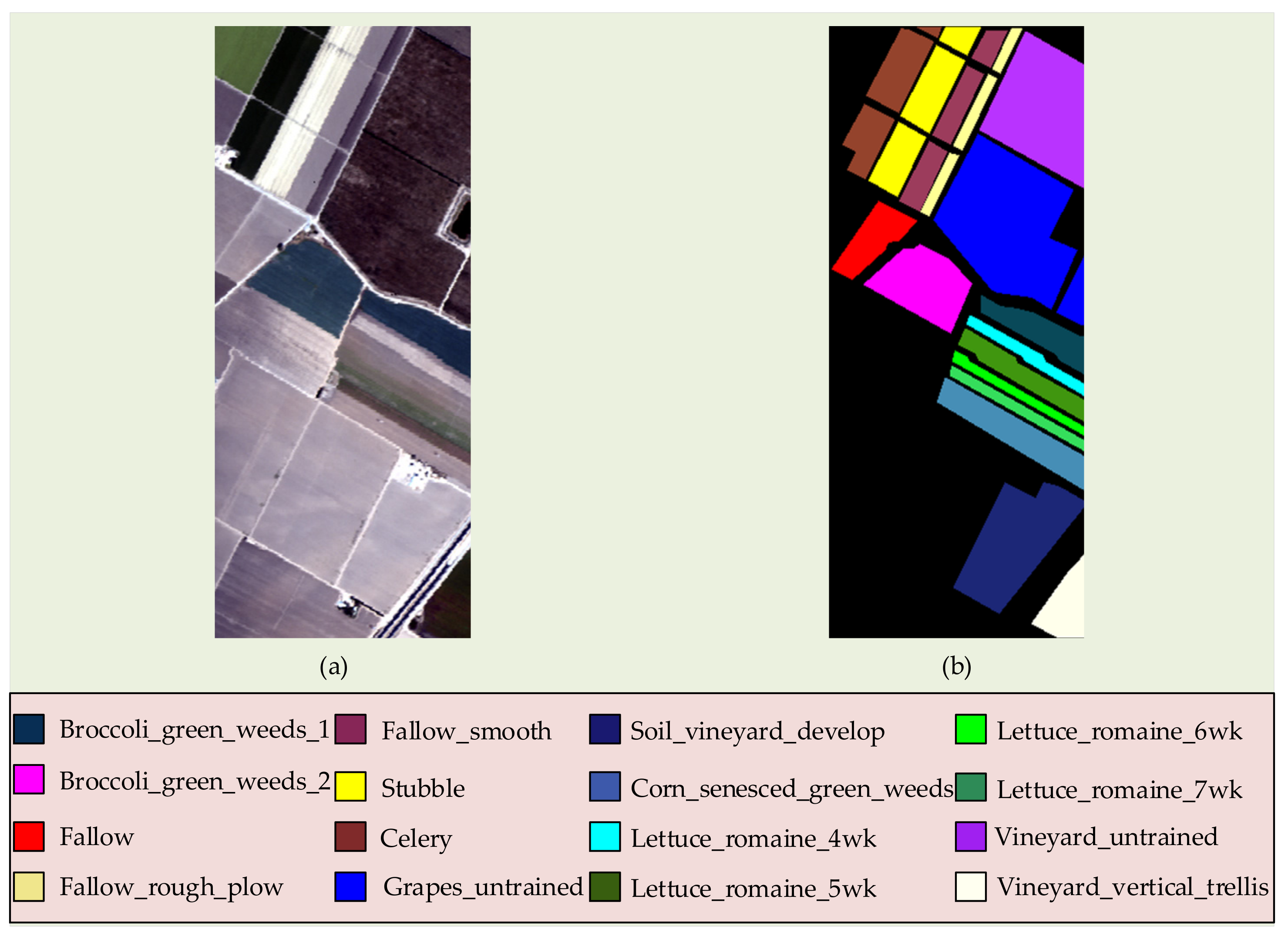
The Xiong’an hyperspectral data were obtained by Airborne Multi-Modular Imaging Spectrometer (AMMIS) in New District, Hebei Province, China. This dataset consists of 512 × 512 pixels and 250 spectral bands. The spatial resolution was 0.5 m, and the spectral band ranged from 400 nm to 1000 nm [50,51,52,53]. All 250 bands were used in the experiments. The original image and the ground reference map of the Xiong’an dataset are shown in Figure 3.

3.2. Experiments on Feature Extraction Methods

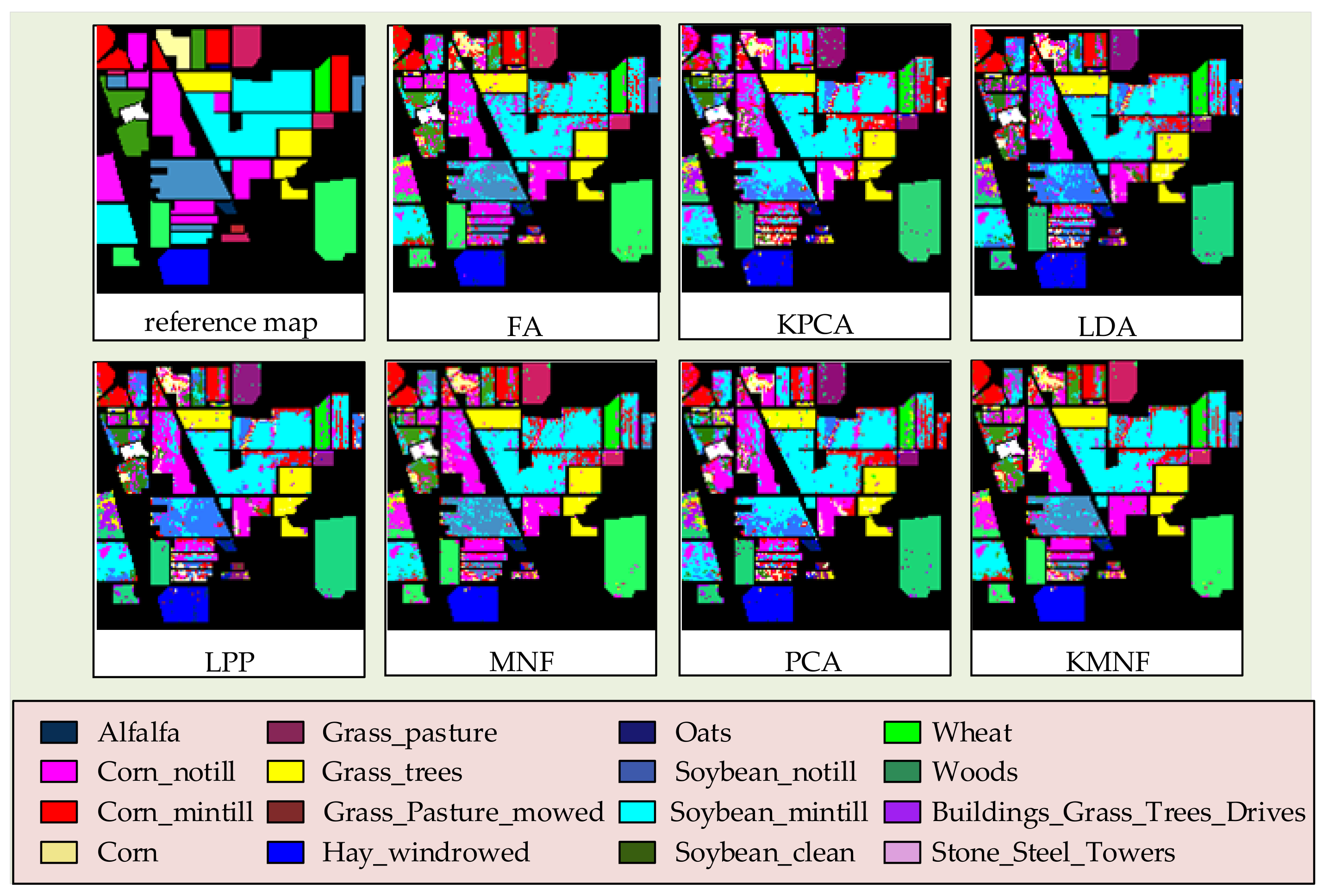
The number of training and testing samples from the Indian Pines, Salinas, and Xiong’an datasets is listed in Table 2 and Table 3. The overall accuracies and confidence intervals for each feature extraction method in terms of SVM classifier are shown in Table 4. The Kappa and confidence intervals for each feature extraction method in terms of the SVM classifier are shown in Table 5. To visualize the classification results, the results of the SVM classifier after applying different methods on the Indian Pines, Xiong’an, and Salinas datasets are depicted in Figure 4, Figure 5, and Figure 6, respectively.
In this experiment, the SVM classifier with RBF kernel was utilized as the classification method, and the overall accuracies and confidence intervals were used to evaluate the results. Experiments using three HSIs with different spatial and spectral resolutions over different scenes were conducted. The results suggest that compared with other methods, the improvements of KMNF transformation in overall accuracies are 2.00%, 1.52%, and 1.06% in the Indian Pines, Salinas, and Xiong’an datasets, respectively, and the improvements of KMNF transformation in Kappa are 2.17%, 1.65%, and 1.08% in the Indian Pines, Salinas, and Xiong’an datasets, respectively. The results demonstrate the excellent performance of KMNF transformation in classification.

3.3. Experiments on Runtimes Testing of Each Method

The runtimes of each feature extraction method with a data size of 100 × 100 × 250 are shown in Table 6.
In this experiment, the runtimes of each feature extraction method were tested with a data size of 100 × 100 × 250 to evaluate the computational complexity. The results illustrate that the KMNF transformation requires more processing time with the same data size, representing that KMNF transformation has higher computational complexity than other feature extraction methods.

3.4. Experiments on GNKMNF Transformation

Two experimental results are described in this section. Section 3.4.1 reports how the experiment was conducted to analyze the sample size selection in NKMNF. Section 3.4.2 reports how the execution efficiency of KMNF transformation, NKMNF transformation, and GNKMNF transformation were evaluated by increasing the data size. In addition, the execution efficiency of GNKMNF is analyzed in detail with a data size of 64 × 64 × 250.

3.4.1. Experiments on Sample Size Selection

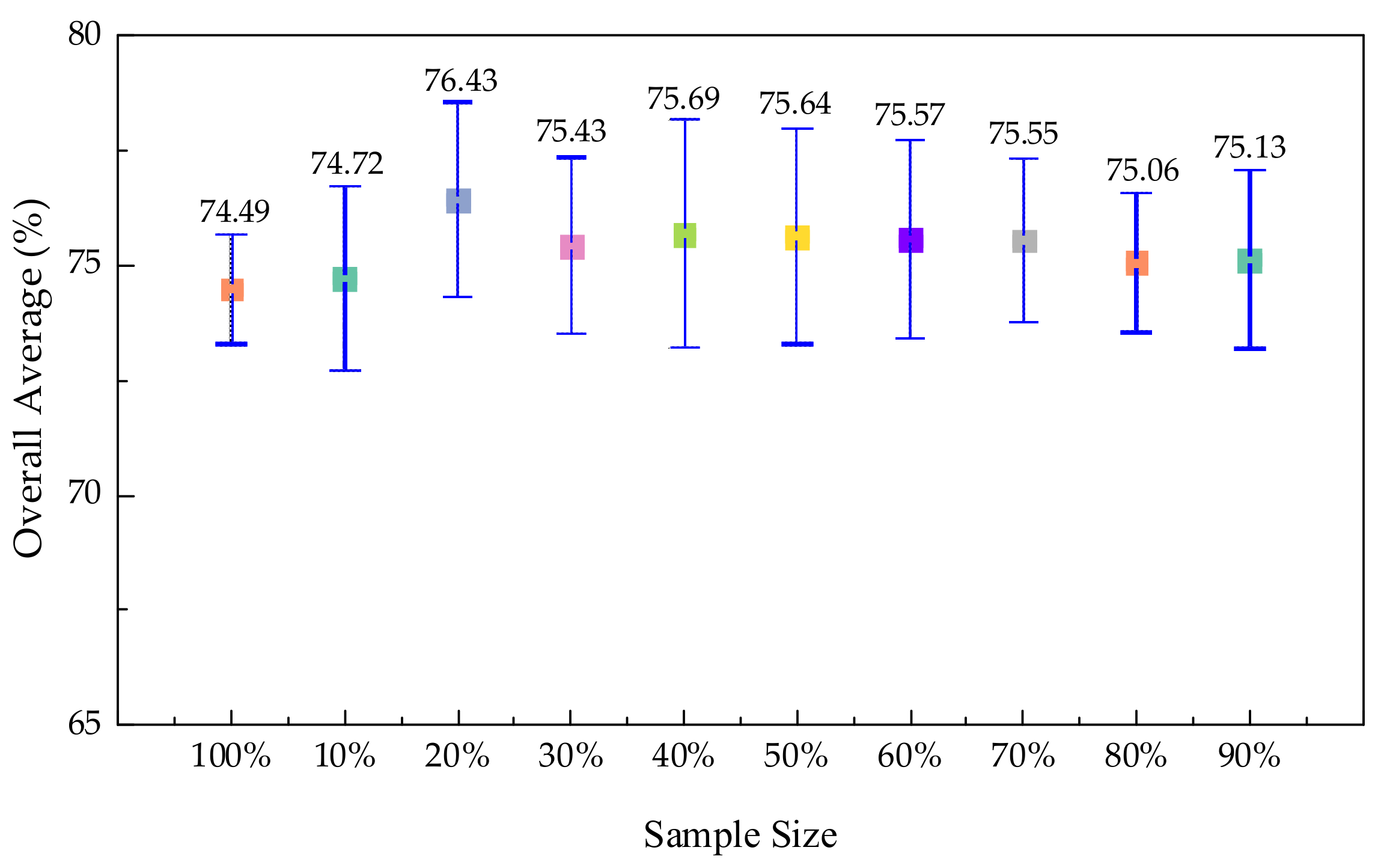
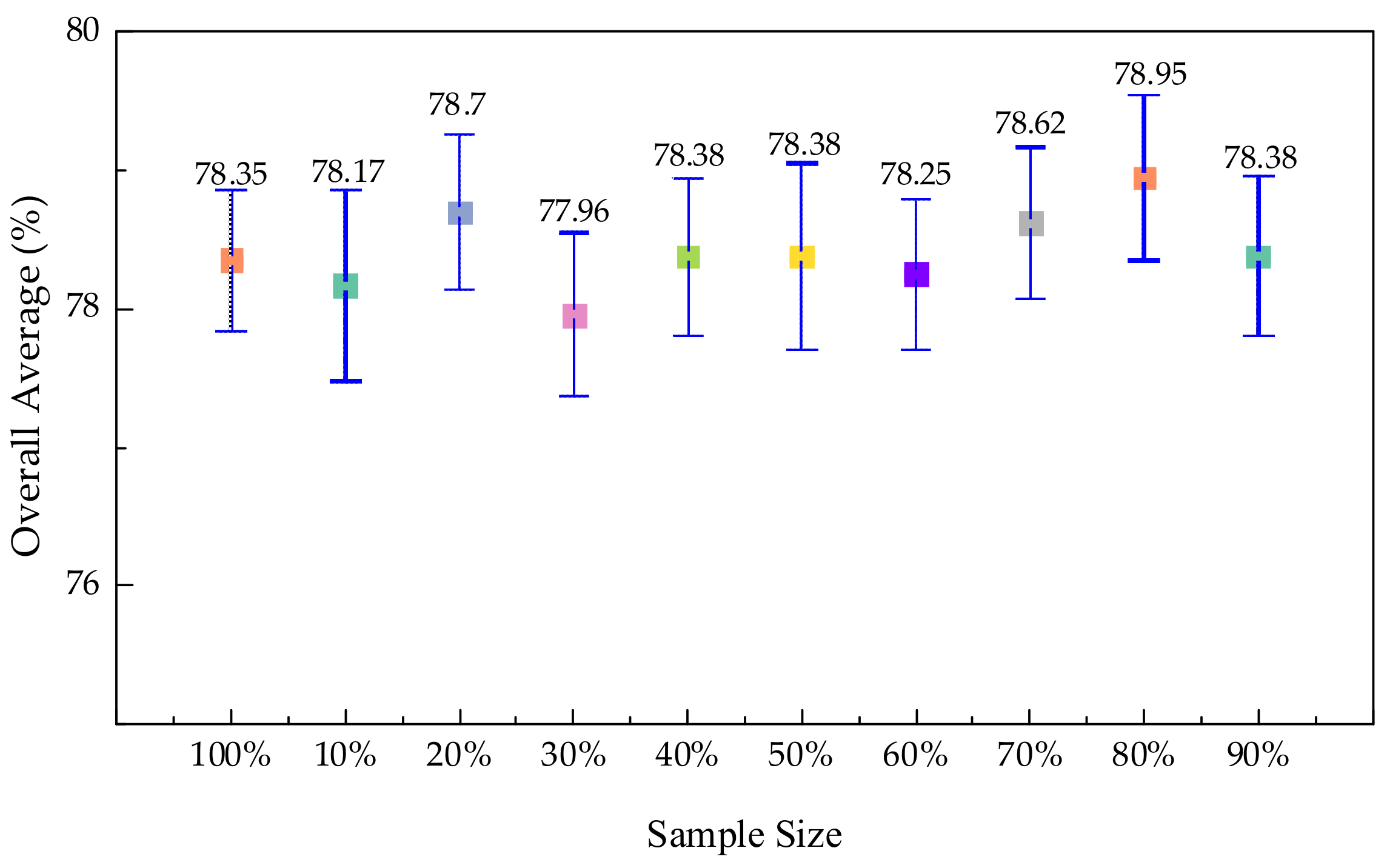
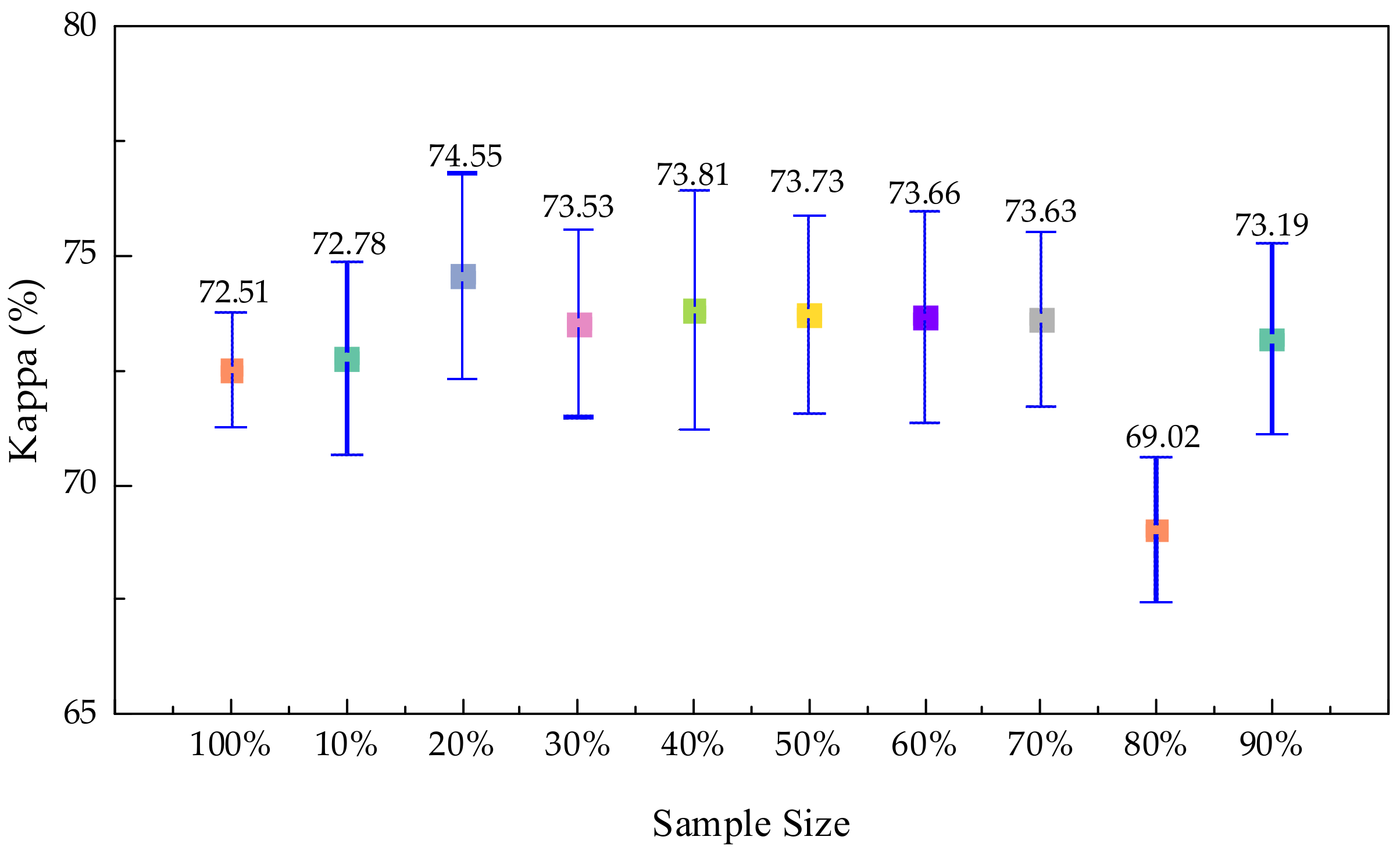
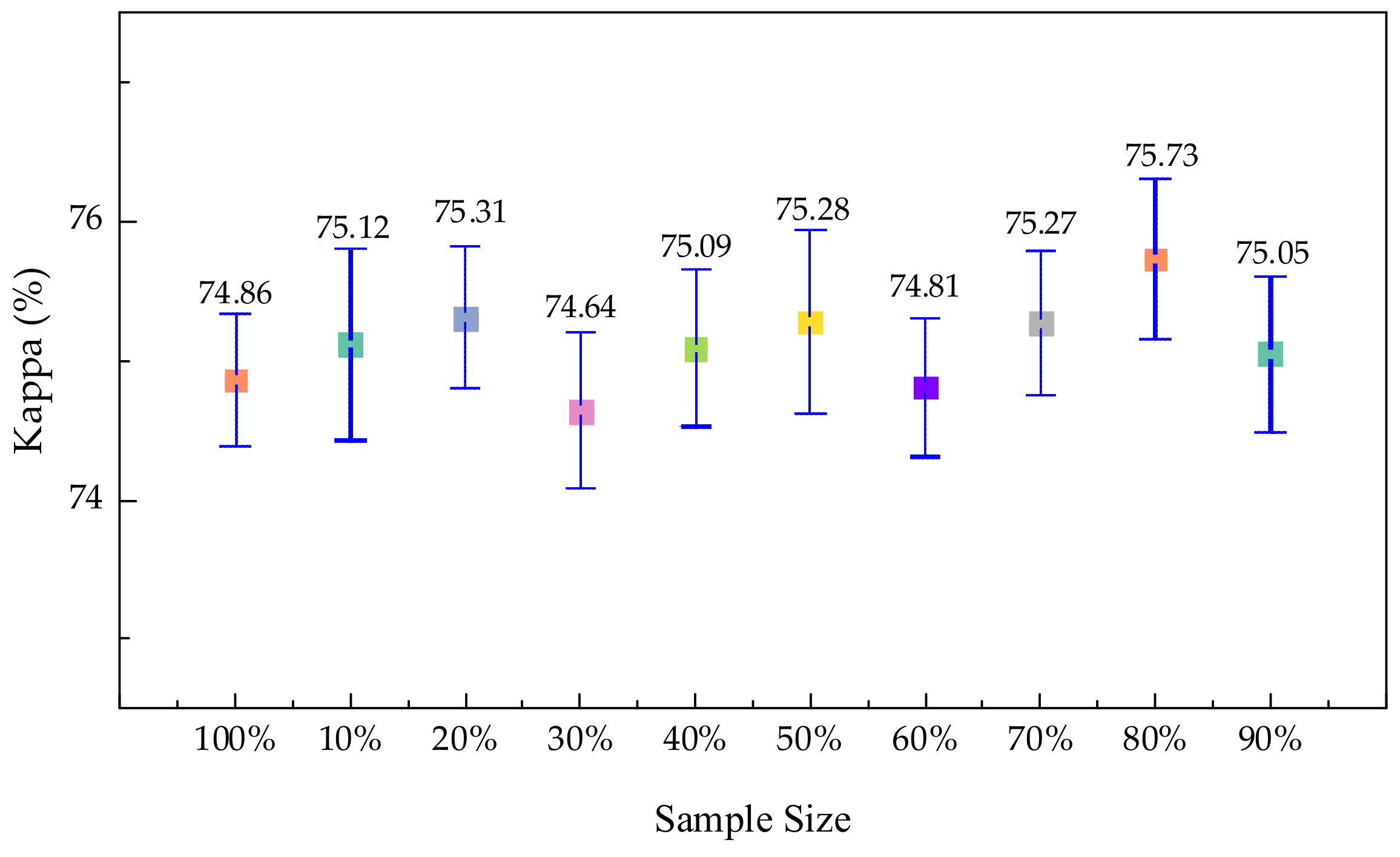
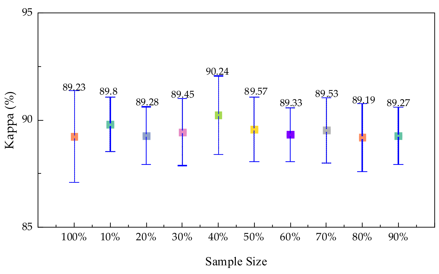
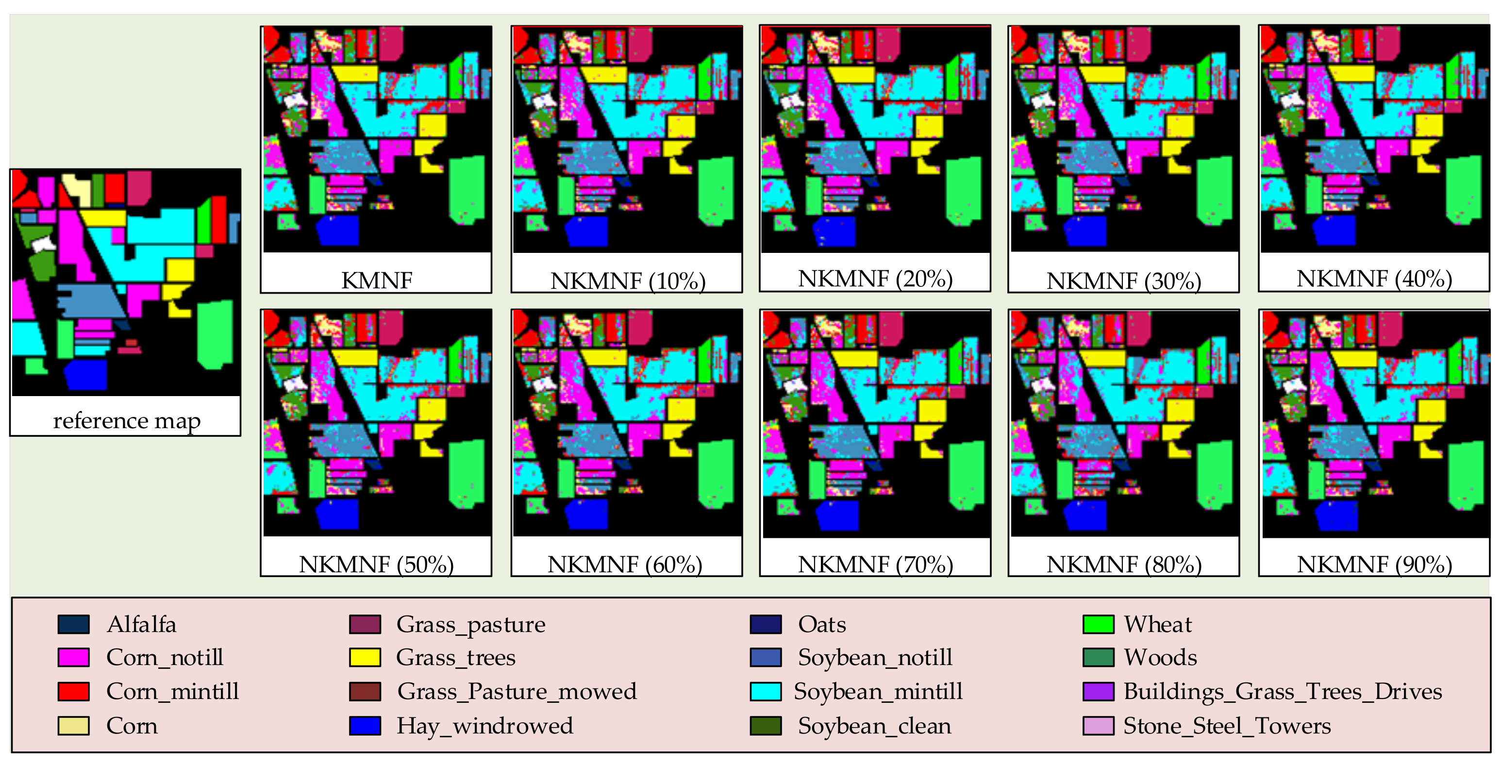
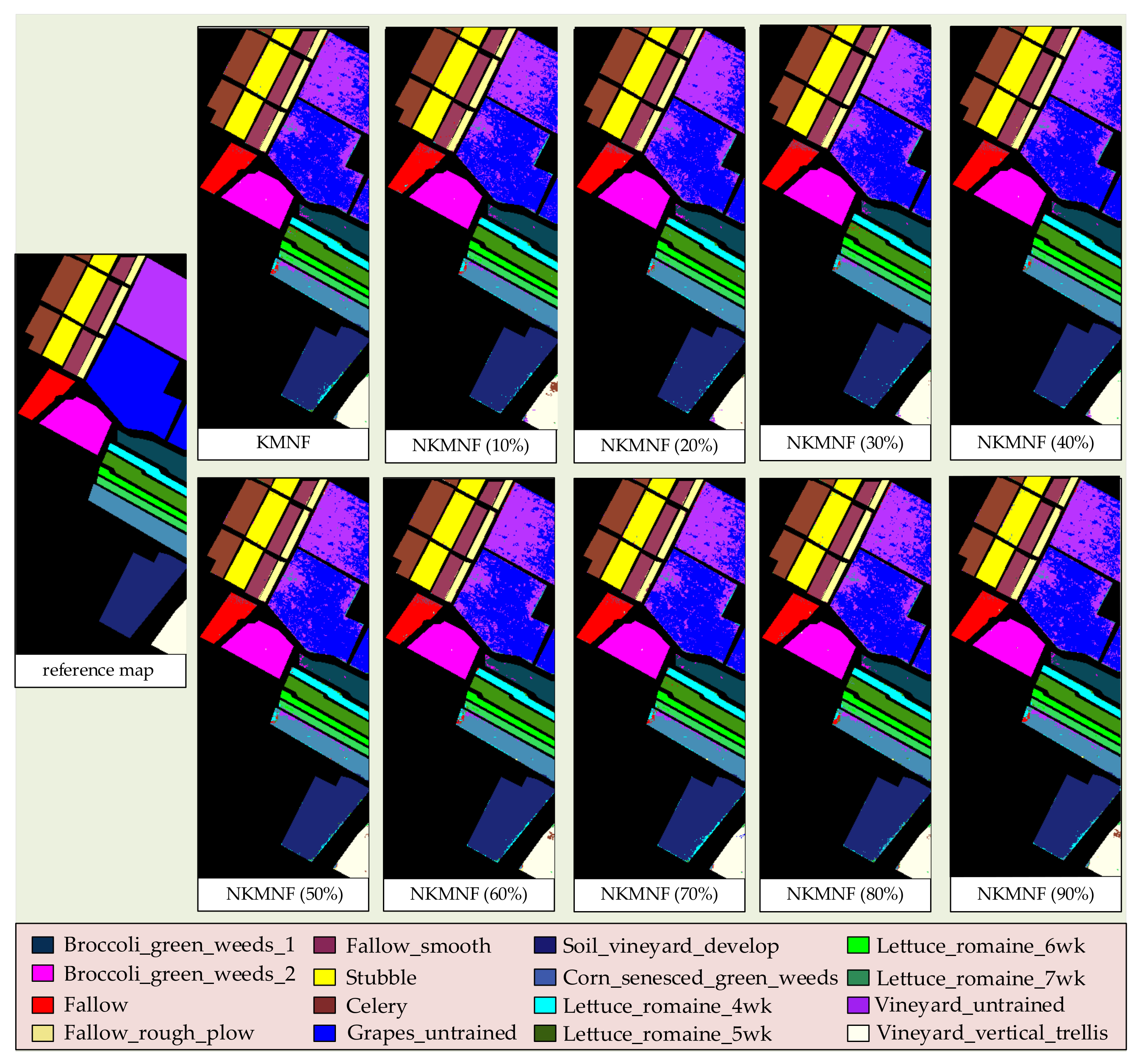
The overall accuracies and confidence intervals of the SVM classifier after NKMNF with different proportion sample sizes in the Indian Pines, Xiong’an, and Salinas datasets are shown in Figure 7, Figure 8, and Figure 9, respectively. The Kappa and confidence intervals of the SVM classifier after NKMNF with different proportion sample sizes in the Indian Pines, Xiong’an, and Salinas datasets are shown in Figure 10, Figure 11, and Figure 12, respectively. In these figures, 100% represents using all pixels, which is the KMNF transformation. To visualize the classification results, the results of SVM classification of the Indian Pines, Xiong’an, and Salinas datasets after NKMNF with different proportion sample sizes are depicted in Figure 13, Figure 14, and Figure 15, respectively.
In this experiment, the overall accuracies, Kappa, and their confidence intervals of the SVM classifier after NKMNF with different proportion sample sizes in the Indian Pines, Xiong’an, and Salinas datasets were evaluated. The results show that NKMNF transformation outperforms KMNF transformation in most cases. Comprehensively considering the performance of NKMNF transformation and the computational complexity of this algorithm, the NKMNF transformation demonstrates the best performance when the proportion of sub-kernel matrix in the entire kernel matrix is 20%.

3.4.2. Experiments on GNKMNF Transformation

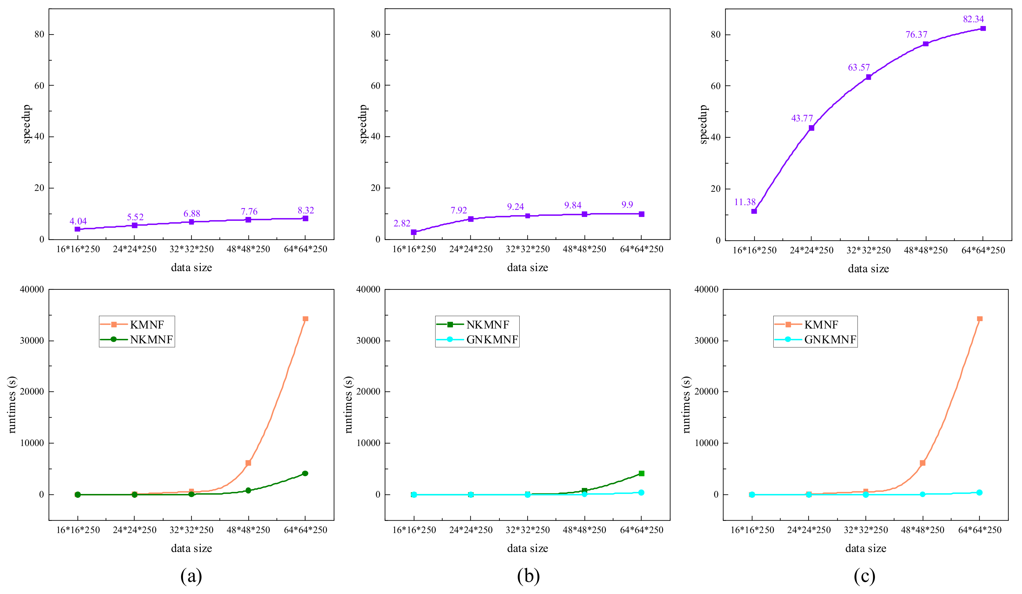
As seen in Section 3.4.1, the NKMNF transformation demonstrates the best performance when the proportion of sub-kernel matrix in the entire kernel matrix is 20%. In this experiment, the proportion 20% was used for testing in NKMNF transformation. A comparison, in terms of computational cost, of the KMNF, NKMNF, and GNKMNF transformations using different data sizes is shown in Figure 16. The detailed analyses of the execution efficiency of GNKMNF with a data size of 64 × 64 × 250 is shown in Table 7.
In this section, the computational costs of KMNF, NKMNF, and GNKMNF transformation with different data volumes were assessed. The results demonstrate that compared with KMNF and NKMNF, the GNKMNF leads to a significant improvement in execution efficiency. In addition, the execution efficiency of GNKMNF with a data size of 64 × 64 × 250 was analyzed in detail and provides a reference for the further research in parallel computing.

4. Discussion

In this section, the four experimental results stated in Section 3 are discussed.
The first experiment was designed to evaluate the performance of each feature extraction method (including PCA, MNF, KPCA, FA, LDA, LPP, and KMNF) in classification. This experiment was conducted on three real HSIs with different spatial and spectral resolutions over different scenes. Taking overall accuracy as the evaluation criterion, the classification performance of each feature extraction method in terms of the SVM classifier with RBF kernel was assessed. The results show that: (1) compared with other feature extraction methods, KMNF has excellent classification performance in terms of overall accuracy. The improvements of KMNF transformation in overall accuracy on the Indian Pines, Salinas, and Xiong’an datasets are 2.00%, 1.52%, and 1.06%, respectively, and the improvements of KMNF transformation in Kappa are 2.17%, 1.65%, and 1.08% in the Indian Pines, Salinas, and Xiong’an datasets, respectively; (2) in most cases, the more features extracted, the higher the overall classification accuracy; (3) MNF and FA can be considered for dimension reduction in practice. The experimental results suggest KMNF outperforms PCA, KPCA, LDA, and LPP and is relatively equivalent to MNF and FA.
The second experiment tested the computational costs of each feature extraction method with a data size of 100 × 100 × 250. This experiment was designed to show the computational complexity of each method intuitively. The results suggest that: (1) with the same data size, the KMNF transformation requires more processing time, which indicates that KMNF has higher computational complexity compared with other algorithms; (2) compared with LPP, KPCA, and KMNF, PCA, MNF, FA, and LDA have lower computational complexity and are more applicable to the processing of large-scale datasets.
The Nyström method estimates the eigenvector of the entire kernel matrix by the decomposition and extrapolation of the sub-kernel matrix. The sample size of the sub-kernel matrix is an essential factor that affects the result of NKMNF. The third experiment was conducted to determine the optimal sample size. The results show that: (1) comprehensively considering the performance of NKMNF and the execution speed of this algorithm, the NKMNF transformation has the best performance when the proportion of sub-kernel matrix in the entire kernel matrix is 20%; (2) in most cases, NKMNF transformation outperforms KMNF in Kappa and overall classification accuracy; (3) with a proportional gradient to select sample sizes in NKMNF transformation, the differentials of NMKNF in overall classification accuracy are 1.71%, 0.98%, and 0.99% in the Indian Pines, Salina, and Xiong’an datasets, respectively, and the differentials of NMKNF in Kappa are 5.53%, 1.50%, and 1.09% in the Indian Pines, Salina, and Xiong’an datasets, respectively.
The last experiment was designed to evaluate the execution efficiency of KMNF, NKMNF, and GNKMNF. By increasing the data volume in processing, the computational costs of KMNF, NKMNF, and GNKMNF were tested. The results suggest that: (1) the larger the data size, the more significant the acceleration effect; (2) when the data size is 64 × 64 × 250, the execution efficiency of NKMNF speeds up by about 8x compared with the KMNF transformation; (3) when the data volume was 64 × 64 × 250, the execution efficiency of GNKMNF speeds up by about 10× and 80× compared with NKMNF transformation and KMNF transformation, respectively.
From the above analysis, it can be seen that compared with other feature extraction methods, KMNF has excellent classification performance in terms of overall accuracy. Although KMNF is a valuable feature extraction method for HSIs, it is found that the KMNF transformation presents the problem of high computational complexity and low execution efficiency. It is not applicable to the processing of large-scale datasets. The Nyström method is an efficient method to solve this problem, and the NKMNF is presented in this paper. Comprehensively considering the performance of NKMNF and the execution speed of the algorithm, the NKMNF transformation demonstrates the best performance when the proportion of sub-kernel matrix in the entire kernel matrix is 20%. Compared with the KMNF transformation, when the data size is 64 × 64 × 250, the execution efficiency of NKMNF and GNKMNF speed up by about 8× and 80×, respectively. The outcome demonstrates the significant performance of GNKMNF in feature extraction and execution efficiency.

5. Conclusions

The KMNF transformation presents the problem of high computational complexity and low execution efficiency. It is not suitable for the processing of large-scale datasets. Therefore, it is valuable to develop a real-time implementation for KMNF transformation. Considering the feature extraction performance and the execution speed, a GPU and Nyström method-based method is presented in this paper. The experimental results demonstrate the significant performance of GNKMNF in execution efficiency and classification. The results can be generalized as follows:
(1) In this paper, the performance of different feature extraction methods (including PCA, MNF, KPCA, FA, LDA, LPP, and KMNF) are evaluated in terms of the Indian Pine, Salinas, and Xiong’an datasets. The experimental results show the generalization and effectiveness of KMNF transformation in feature extraction, which provides a reference for further research in feature extraction.
(2) In terms of high computational complexity and low execution efficiency in KMNF transformation, the Nyström method is employed in this paper. The experimental results demonstrate that the NKMNF transformation has lower computational complexity and achieves satisfactory results in classification. The proposed framework can be developed as a general model for the real-time implementation of other algorithms.
(3) Comprehensively considering the performance of NKMNF and the execution speed of this algorithm, the NKMNF transformation demonstrates the best performance when the proportion of sub-kernel matrix in the entire kernel matrix is 20%.
(4) GPU parallel computing is employed to improve the execution efficiency of NKMNF further. Experimental results show that with a data size of 64 × 64 × 250, the GNKMNF speeds up by about 80× compared with KMNF.
In summary, the results show that the GNKMNF demonstrates a significant performance in classification and execution efficiency. The realization of this method can provide a reference for fast algorithm design of other feature extraction methods. In recent years, deep learning architectures have become an exciting research topic in feature extraction. In the future, we are interested in exploring a lightweight deep learning framework to extract the nonlinear feature structures in HSIs.

Author Contributions

Conceptualization, T.X. and Y.W.; methodology, T.X.; software, T.X.; validation, T.X. and X.D.; formal analysis, T.X.; investigation, T.X.; resources, Y.W.; data curation, T.X. and Y.W.; writing—original draft preparation, T.X.; writing—review and editing, T.X. and Y.W.; visualization, X.D.; supervision, Y.W.; project administration, Y.W.; funding acquisition, Y.W. All authors have read and agreed to the published version of the manuscript.

Funding

This research was funded by National Natural Science Foundation of China (61627804), and National Civil Aerospace Project (No. D040102).

Institutional Review Board Statement

Not applicable.

Informed Consent Statement

Not applicable.

Data Availability Statement

The Xiong’an dataset used in this paper can be downloaded from http://www.hrs-cas.com/a/share/shujuchanpin/2019/0501/1049.html (accessed on 20 December 2021).

Acknowledgments

We are grateful to the State Key Laboratory of Remote Sensing Science, Institute of Remote Sensing and Digital Earth, Chinese Academy of Sciences, who provided the Xiong’an hyperspectral dataset for this research.

Conflicts of Interest

The authors declare no conflict of interest.

References

  1. Falco, N.; Benediktsson, J.A.; Bruzzone, L. A study on the effectiveness of different independent component analysis algorithms for hyperspectral image classification. IEEE J. Sel. Top. Appl. Earth Obs. Remote Sens. 2014, 7, 2183–2199. [Google Scholar] [CrossRef]
  2. Zhou, Y.; Peng, J.; Chen, C.L.P. Dimension Reduction Using Spatial and Spectral Regularized Local Discriminant Embedding for Hyperspectral Image Classification. IEEE Trans. Geosci. Remote Sens. 2015, 53, 1082–1095. [Google Scholar] [CrossRef]
  3. Harsanyi, J.C.; Chang, C.-I. Hyperspectral image classification and dimensionality reduction: An orthogonal subspace projection approach. IEEE Trans. Geosci. Remote Sens. 1994, 32, 779–785. [Google Scholar] [CrossRef] [Green Version]
  4. Yuan, Y.; Zheng, X.; Lu, X. Discovering Diverse Subset for Unsupervised Hyperspectral Band Selection. IEEE Trans. Image Process. 2017, 26, 51–64. [Google Scholar] [CrossRef]
  5. Dong, Y.; Du, B.; Zhang, L.; Zhang, L. Dimensionality Reduction and Classification of Hyperspectral Images Using Ensemble Discriminative Local Metric Learning. IEEE Trans. Geosci. Remote Sens. 2017, 55, 2509–2524. [Google Scholar] [CrossRef]
  6. Xue, T.; Wang, Y.; Chen, Y.; Jia, J.; Wen, M.; Guo, R.; Wu, T.; Deng, X. Mixed Noise Estimation Model for Optimized Kernel Minimum Noise Fraction Transformation in Hyperspectral Image Dimensionality Reduction. Remote Sens. 2021, 13, 2607. [Google Scholar] [CrossRef]
  7. Sun, W.; Du, Q. Hyperspectral band selection: A review. IEEE Geosci. Remote Sens. Mag. 2019, 7, 118–139. [Google Scholar] [CrossRef]
  8. Yin, J.; Wang, Y.; Zhao, Z. Optimal Band Selection for Hyperspectral Image Classification Based on Inter-Class Separability. In Proceedings of the 2010 Symposium on Photonics and Optoelectronics, Chengdu, China, 19–21 June 2010; pp. 1–4. [Google Scholar] [CrossRef]
  9. Sildomar, T.-M.; Yukio, K. A Particle Swarm Optimization-Based Approach for Hyperspectral Band Selection. In Proceedings of the 2007 IEEE Congress on Evolutionary Computation, Singapore, 25–28 September 2007; pp. 3335–3340. [Google Scholar] [CrossRef]
  10. Wang, Q.; Lin, J.; Yuan, Y. Salient band selection for hyperspectral image classification via manifold ranking. IEEE Trans. Neural Netw. Learn. Syst. 2016, 27, 1279–1289. [Google Scholar] [CrossRef]
  11. Keshava, N. Distance metrics and band selection in hyperspectral processing with applications to material identification and spectral libraries. IEEE Trans. Geosci. Remote Sens. 2004, 42, 1552–1565. [Google Scholar] [CrossRef]
  12. Su, H.; Du, Q.; Chen, G.; Du, P. Optimized hyperspectral band selection using particle swarm optimization. IEEE J. Sel. Top. Appl. Earth Obs. Remote Sens. 2014, 7, 2659–2670. [Google Scholar] [CrossRef]
  13. Chang, C.-I.; Du, Q.; Sun, T.-L.; Althouse, M. A joint band prioritization and band-decorrelation approach to band selection for hyperspectral image classification. IEEE Trans. Geosci. Remote Sens. 1999, 37, 2631–2641. [Google Scholar] [CrossRef] [Green Version]
  14. Bajcsy, P.; Groves, P. Methodology for hyperspectral band selection. Photogramm. Eng. Remote Sens. 2004, 70, 793–802. [Google Scholar] [CrossRef]
  15. Yang, H.; Du, Q.; Su, H.; Sheng, Y. An efficient method for supervised hyperspectral band selection. IEEE Geosci. Remote Sens. Lett. 2010, 8, 138–142. [Google Scholar] [CrossRef]
  16. Martínez-Usómartinez-Uso, A.; Pla, F.; Sotoca, J.M.; García-Sevilla, P. Clustering-based hyperspectral band selection using information measures. IEEE Trans. Geosci. Remote Sens. 2007, 45, 4158–4171. [Google Scholar] [CrossRef]
  17. Cariou, C.; Chehdi, K.; Le Moan, S. BandClust: An unsupervised band reduction method for hyperspectral remote sensing. IEEE Geosci. Remote Sens. Lett. 2010, 8, 565–569. [Google Scholar] [CrossRef]
  18. Zhang, M.; Ma, J.; Gong, M. Unsupervised hyperspectral band selection by fuzzy clustering with particle swarm optimization. IEEE Geosci. Remote Sens. Lett. 2017, 14, 773–777. [Google Scholar] [CrossRef]
  19. Li, J.-M.; Qian, Y.-T. Clustering-based hyperspectral band selection using sparse nonnegative matrix factorization. J. Zhejiang Univ. Sci. C 2011, 12, 542–549. [Google Scholar] [CrossRef]
  20. Li, S.; Qi, H. Sparse Representation-Based Band Selection for Hyperspectral Images. In Proceedings of the 18th IEEE International Conference on Image Processing, Brussels, Belgium, 11–14 September 2011; pp. 2693–2696. [Google Scholar] [CrossRef]
  21. Sun, W.; Zhang, L.; Du, B.; Li, W.; Lai, Y.M. Band selection using improved sparse subspace clustering for hyperspectral imagery classification. IEEE J. Sel. Top. Appl. Earth Obs. Remote Sens. 2015, 8, 2784–2797. [Google Scholar] [CrossRef]
  22. Gao, L.; Zhao, B.; Jia, X.; Liao, W.; Zhang, B. Optimized kernel minimum noise fraction transformation for hyperspectral image classification. Remote Sens. 2017, 9, 548. [Google Scholar] [CrossRef] [Green Version]
  23. Roger, R.E. Principal Components transform with simple, automatic noise adjustment. Int. J. Remote Sens. 1996, 17, 2719–2727. [Google Scholar] [CrossRef]
  24. Green, A.; Berman, M.; Switzer, P.; Craig, M. A transformation for ordering multispectral data in terms of image quality with implications for noise removal. IEEE Trans. Geosci. Remote Sens. 1988, 26, 65–74. [Google Scholar] [CrossRef] [Green Version]
  25. Bandos, T.V.; Bruzzone, L.; Camps-Valls, G. Classification of hyperspectral images with regularized linear discriminant analysis. IEEE Trans. Geosci. Remote Sens. 2009, 47, 862–873. [Google Scholar] [CrossRef]
  26. Casalino, G.; Gillis, N. Sequential dimensionality reduction for extracting localized features. Pattern Recognit. 2017, 63, 15–29. [Google Scholar] [CrossRef] [Green Version]
  27. Berry, M.; Browne, M.; Langville, A.N.; Pauca, V.P.; Plemmons, R.J. Algorithms and applications for approximate nonnegative matrix factorization. Comput. Stat. Data Anal. 2007, 52, 155–173. [Google Scholar] [CrossRef] [Green Version]
  28. Nielsen, A.A. Kernel maximum autocorrelation factor and minimum noise fraction transformations. IEEE Trans. Image Process. 2010, 20, 612–624. [Google Scholar] [CrossRef] [Green Version]
  29. Schölkopf, B.; Smola, A.J.; Müller, K.-R. Kernel Principal Component Analysis. In Transactions on Petri Nets and Other Models of Concurrency XV; Springer Science and Business Media LLC: Berlin, Germany, 1997; pp. 583–588. [Google Scholar]
  30. Jia, X.; Kuo, B.-C.; Crawford, M.M. Feature mining for hyperspectral image classification. Proc. IEEE 2013, 101, 676–697. [Google Scholar] [CrossRef]
  31. Wong, W.K.; Zhao, H. Supervised optimal locality preserving projection. Pattern Recognit. 2012, 45, 186–197. [Google Scholar] [CrossRef]
  32. Roweis, S.T. Nonlinear Dimensionality Reduction by Locally Linear Embedding. Science 2000, 290, 2323–2326. [Google Scholar] [CrossRef] [PubMed] [Green Version]
  33. Chen, P.; Jiao, L.; Liu, F.; Gou, S.; Zhao, J.; Zhao, Z. Dimensionality reduction of hyperspectral imagery using sparse graph learning. IEEE J. Sel. Top. Appl. Earth Obs. Remote Sens. 2016, 10, 1165–1181. [Google Scholar] [CrossRef]
  34. Gillis, N.; Plemmons, R.J. Sparse nonnegative matrix underapproximation and its application to hyperspectral image analysis. Linear Algebra Its Appl. 2013, 438, 3991–4007. [Google Scholar] [CrossRef]
  35. Bachmann, C.; Ainsworth, T.; Fusina, R. Exploiting manifold geometry in hyperspectral imagery. IEEE Trans. Geosci. Remote Sens. 2005, 43, 441–454. [Google Scholar] [CrossRef]
  36. Kumar, B.; Dikshit, O.; Gupta, A.; Singh, M.K. Feature extraction for hyperspectral image classification: A review. Int. J. Remote Sens. 2020, 41, 6248–6287. [Google Scholar] [CrossRef]
  37. Lu, X.; Yang, D.; Jia, F.; Yang, Y.; Zhang, L. Hyperspectral Image Classification Based on Multilevel Joint Feature Extraction Network. IEEE J. Sel. Top. Appl. Earth Obs. Remote Sens. 2021, 14, 10977–10989. [Google Scholar] [CrossRef]
  38. Li, Z.; Huang, H.; Zhang, Z.; Shi, G. Manifold-Based Multi-Deep Belief Network for Feature Extraction of Hyperspectral Image. Remote Sens. 2022, 14, 1484. [Google Scholar] [CrossRef]
  39. Chen, Y.S.; Jiang, H.L.; Li, C.Y.; Jia, X.P.; Ghamisi, P. Deep Feature Extraction and Classification of Hyperspectral Images Based on Convolutional Neural Networks. IEEE Trans. Geosci. Remote Sens. 2016, 54, 6232–6251. [Google Scholar] [CrossRef] [Green Version]
  40. Feng, J. Attention multibranch convolutional neural network for hyperspectral image classification based on adaptive region search. IEEE Trans. Geosci. Remote Sens. 2021, 59, 5054–5070. [Google Scholar] [CrossRef]
  41. Mou, L.; Zhu, X.X. Learning to pay attention on spectral domain: A spectral attention module-based convolutional network for hyperspectral image classification. IEEE Trans. Geosci. Remote Sens. 2020, 58, 110–122. [Google Scholar] [CrossRef]
  42. Xue, Z.; Zhang, M.; Liu, Y.; Du, P. Attention-based second-order pooling network for hyperspectral image classification. IEEE Trans. Geosci. Remote Sens. 2021, 59, 9600–9615. [Google Scholar] [CrossRef]
  43. Li, Z.Y.; Huang, H.; Li, Y.; Pan, Y.S. M3DNet: A manifold-based discriminant feature learning network for hyperspectral imagery. Expert Syst. Appl. 2020, 144, 113089. [Google Scholar] [CrossRef]
  44. Li, W.; Prasad, S.; Fowler, J.E. Decision Fusion in Kernel-Induced Spaces for Hyperspectral Image Classification. IEEE Trans. Geosci. Remote Sens. 2014, 52, 3399–3411. [Google Scholar] [CrossRef] [Green Version]
  45. Shawe-Taylor, J.; Cristianini, N. Kernel Methods for Pattern Analysis; Cambridge University Press: New York, NY, USA, 2004. [Google Scholar]
  46. Rasti, B.; Scheunders, P.; Ghamisi, P.; Licciardi, G.; Chanussot, J. Noise reduction in hyperspectral imagery: Overview and application. Remote Sens. 2018, 10, 482. [Google Scholar] [CrossRef] [Green Version]
  47. Nielsen, A.A. An Extension to a Filter Implementation of a Local Quadratic Surface for Image Noise Estimation. In Proceedings of the 10th International Conference on Image Analysis and Processing, Venice, Italy, 27–29 September 1999; pp. 119–124. [Google Scholar] [CrossRef] [Green Version]
  48. Williams, C.; Seeger, M. Using the Nyström method to speed up kernel machines. In Proceedings of the 14th Annual Conference on Neural Information Processing Systems, Denver, CO, USA, 1 January 2001; pp. 682–688. [Google Scholar]
  49. Barrachina, S.; Castillo, M.; Igual, F.D.; Mayo, R.; Quintana-Ortí, E.S.; Quintana-Ortí, G. Exploiting the capabilities of modern GPUs for dense matrix computations. Concurr. Comput. Pract. Exp. 2009, 21, 2457–2477. [Google Scholar] [CrossRef]
  50. Jia, J.; Wang, Y.; Cheng, X.; Yuan, L.; Zhao, D.; Ye, Q.; Zhuang, X.; Shu, R.; Wang, J. Destriping algorithms based on statistics and spatial filtering for visible-to-thermal infrared pushbroom hyperspectral imagery. IEEE Trans. Geosci. Remote Sens. 2019, 57, 4077–4091. [Google Scholar] [CrossRef]
  51. Jia, J.; Zheng, X.; Guo, S.; Wang, Y.; Chen, J. Removing stripe noise based on improved statistics for hyperspectral images. IEEE Geosci. Remote Sens. Lett. 2020, 19, 1–5. [Google Scholar] [CrossRef]
  52. Cen, Y.; Zhang, L.; Zhang, X.; Wang, Y.; Qi, W.; Tang, S.; Zhang, P. Aerial hyperspectral remote sensing classification dataset of Xiong’an new area (Matiwan Village). J. Remote Sens. 2020, 24, 1299–1306. [Google Scholar] [CrossRef]
  53. Jia, J.; Chen, J.; Zheng, X.; Wang, Y.; Guo, S.; Sun, H.; Jiang, C.; Karjalainen, M.; Karila, K.; Duan, Z.; et al. Tradeoffs in the spatial and spectral resolution of airborne hyperspectral imaging systems: A crop identification case study. IEEE Trans. Geosci. Remote Sens. 2022, 60, 5510918. [Google Scholar] [CrossRef]
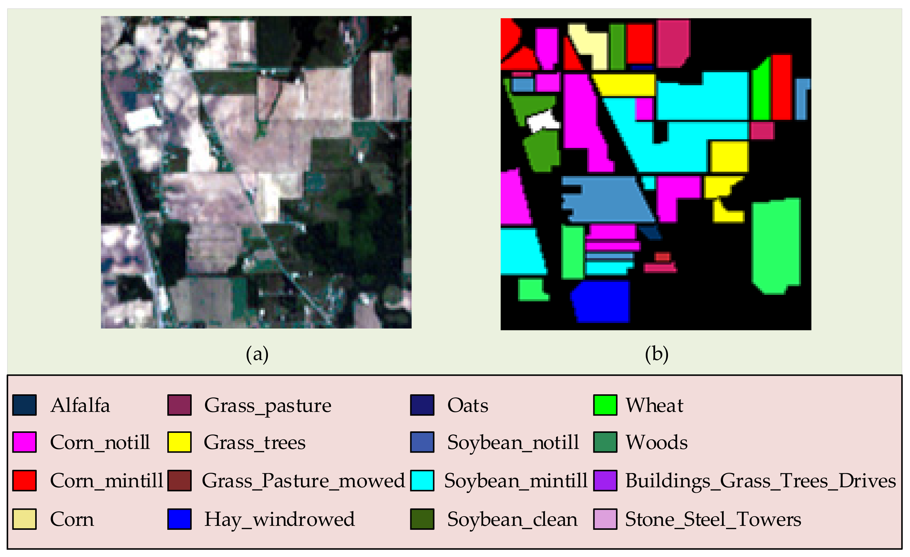
Figure 1. (a) original Indian Pines image; (b) ground reference map of Indian Pines.
Remotesensing 14 01737 g001
Figure 2. (a) original Salinas image; (b) ground reference map of Salinas.
Remotesensing 14 01737 g002
Figure 3. (a) original Xiong’an image; (b) ground reference map of Xiong’an.
Remotesensing 14 01737 g003
Figure 4. The results of SVM classifier for Indian Pines after each feature extraction method (number of features = 45).
Remotesensing 14 01737 g004
Figure 5. The results of SVM classifier for Xiong’an after each feature extraction method (number of features = 45).
Remotesensing 14 01737 g005
Figure 6. The results of SVM classifier for Salinas after each feature extraction method (number of features = 45).
Remotesensing 14 01737 g006
Figure 7. The overall accuracies and confidence intervals of SVM classifier after NKMNF with different proportion sample sizes (number of features = 45) in Indian Pines.
Remotesensing 14 01737 g007
Figure 8. The overall accuracies and confidence intervals of SVM classifier after NKMNF with different proportion sample sizes (number of features = 45) in Xiong’an.
Remotesensing 14 01737 g008
Figure 9. The overall accuracies and confidence intervals of SVM classifier after NKMNF with different proportion sample sizes (number of features = 45) in Salinas.
Remotesensing 14 01737 g009
Figure 10. The Kappa and confidence intervals of SVM classifier after NKMNF with different proportion sample sizes (number of features = 45) in Indian Pines.
Remotesensing 14 01737 g010
Figure 11. The Kappa and confidence intervals of SVM classifier after NKMNF with different proportion sample sizes (number of features = 45) in Xiong’an.
Remotesensing 14 01737 g011
Figure 12. The Kappa and confidence intervals of SVM classifier after NKMNF with different proportion sample sizes (number of features = 45) in Salinas.
Remotesensing 14 01737 g012
Figure 13. The results of SVM classifier for Indian Pines after NKMNF with different proportion sample sizes (number of features = 45).
Remotesensing 14 01737 g013
Figure 14. The results of SVM classifier for Xiong’an after NKMNF with different proportion sample sizes (number of features = 45).
Remotesensing 14 01737 g014
Figure 15. The results of SVM classifier for Salinas after NKMNF with different proportion sample sizes (number of features = 45).
Remotesensing 14 01737 g015
Figure 16. Computational cost comparisons for KMNF transformation, NKMNF transformation, and GNKMNF transformation with different data volumes. (a) Computational cost comparison of KMNF transformation and NKMNF transformation; (b) Computational cost comparison of NKMNF transformation and GNKMNF transformation; (c) Computational cost comparison of KMNF transformation and GNKMNF transformation.
Remotesensing 14 01737 g016
Table 1. Hardware parameters of the NVIDIA GeforceGTX745.
ParameterGeForce GTX 745
CUDA Cores384
Clock Rate1.03 GHz
Memory Bus Width128 bit
Global Memory4096 MBytes
Shared Memory49,152 bytes
Constant Memory65,536 bytes
Table 2. Training and testing samples used in Indian Pines and Salinas datasets.
ClassesIndian PinesClassesSalinas
TrainingTestingTrainingTesting
Alfalfa1234Broccoli_green_weeds_15021507
Corn_notill3571071Broccoli_green_weeds_29322794
Corn_mintill208622Fallow4941482
Corn59178Fallow_rough_plow3491045
Grass_pasture121362Fallow_smooth6702008
Grass_trees183547Stubble9902969
Grass_pasture_mowed721Celery8952684
Hay_windrowed120358Grapes_untrained28188453
Oats515Soil_vineyard_develop15514652
Soybean_notill243729Corn_senesced_green_weeds8202458
Soybean_mintill6141841Lettuce_romaine_4wk267801
Soybean_clean148445Lettuce_romaine_5wk4821445
Wheat51154Lettuce_romaine_6wk229687
Woods316949Lettuce_romaine_7wk268802
Builings_Grass_Trees_Drives97289Vineyard_untrained18175451
Stone_Steel_Towers2370Vineyard_vertical_trellis4521355
Table 3. Training and testing samples used in Xiong’an dataset.
ClassesTrainingTesting
Corn21,12463,372
Soybean26427921
Pear_trees326977
Grassland692620,777
Sparsewood23236969
Robinia644019,321
Paddy750722,522
Populus13844150
Sophora japonica203608
Peach_trees3751123
Table 4. The overall accuracies and confidence intervals of SVM classifier after each feature extraction method.
MethodsPCAMNFKPCAFALDALPPKMNF
Indian Pines
3 47.63   ±   4.37 56.71   ±   0.82 50.04   ±   0.25 55.01   ±   1.72 50.34   ±   0.46 49.60   ±   1.07 57.95   ±   1.93
4 50.57   ±   4.44 60.31   ±   1.36 52.83   ±   0.19 57.35   ±   1.21 51.02   ±   0.84 52.37   ±   1.62 60.72   ±   3.98
5 51.48   ±   4.28 61.52   ±   0.60 53.65   ±   0.84 60.09   ±   0.05 53.33   ±   2.39 53.03   ±   1.42 61.63   ±   2.76
10 59.25   ±   1.06 65.47   ±   0.82 57.84   ±   0.88 67.13   ±   0.11 59.79   ±   0.33 62.72   ±   0.56 67.95   ±   2.14
15 62.41   ±   1.15 68.82   ±   0.10 58.49   ±   0.62 69.53   ±   0.32 61.74   ±   0.31 64.98   ±   1.11 69.67   ±   1.06
20 62.78   ±   2.08 68.67   ±   0.90 59.42   ±   0.88 71.07   ±   0.16 63.23   ±   0.49 65.00   ±   1.70 71.97   ±   1.67
25 63.46   ±   1.85 69.72   ±   1.57 60.35   ±   1.52 72.41   ±   1.35 63.86   ±   1.07 65.80   ±   2.27 72.63   ±   1.74
30 63.96   ±   1.39 70.35   ±   1.75 61.98   ±   0.02 73.17   ±   1.55 65.08   ±   1.70 67.14   ±   2.05 75.17   ±   2.15
35 64.10   ±   1.56 70.65   ±   1.71 62.17   ±   0.38 73.70   ±   2.00 66.34   ±   2.54 67.98   ±   2.22 74.66   ±   1.82
40 64.57   ±   1.84 72.81   ±   1.65 62.54   ±   0.06 73.35   ±   2.64 66.60   ±   2.43 68.21   ±   2.10 73.65   ±   1.93
45 64.74   ±   1.61 72.38   ±   2.24 62.27   ±   0.77 73.23   ±   2.88 67.07   ±   2.04 69.64   ±   1.30 74.49   ±   1.20
Salinas
3 79.66   ±   0.95 84.57   ±   0.86 74.54   ±   0.17 80.91   ±   0.29 82.53   ±   0.89 80.42   ±   0.49 86.09   ±   1.07
4 80.74   ±   0.81 85.54   ±   1.22 76.98   ±   0.17 85.42   ±   1.11 82.31   ±   0.98 82.46   ±   1.03 86.27   ±   1.10
5 82.45   ±   0.60 85.86   ±   0.79 79.88   ±   0.19 85.42   ±   1.08 83.50   ±   1.18 82.71   ±   0.94 86.71   ±   0.93
10 85.50   ±   1.19 88.80   ±   0.39 82.01   ±   0.10 86.33   ±   1.20 84.55   ±   1.38 84.22   ±   0.99 89.15   ±   1.40
15 85.40   ±   1.28 88.81   ±   0.46 82.92   ±   0.24 86.45   ±   1.20 85.15   ±   1.42 84.62   ±   1.48 89.44   ±   1.33
20 85.98   ±   1.29 89.16   ±   0.72 84.26   ±   0.03 86.68   ±   1.81 85.94   ±   1.17 85.80   ±   1.41 89.67   ±   1.36
25 86.05   ±   1.28 89.11   ±   0.76 84.51   ±   0.26 88.03   ±   1.35 85.96   ±   1.34 86.58   ±   1.17 89.85   ±   1.62
30 85.96   ±   1.38 89.22   ±   0.85 85.28   ±   0.35 87.45   ±   1.94 85.88   ±   1.23 86.64   ±   1.35 90.04   ±   1.77
35 85.92   ±   1.35 89.11   ±   0.92 85.47   ±   0.37 87.09   ±   2.29 85.75   ±   1.29 86.58   ±   1.37 89.98   ±   1.79
40 85.77   ±   1.46 89.04   ±   0.90 85.76   ±   0.59 88.11   ±   1.83 85.89   ±   1.33 86.57   ±   1.26 90.09   ±   2.04
45 85.99   ±   1.47 89.04   ±   0.84 85.71   ±   0.61 88.34   ±   1.67 85.86   ±   1.33 86.64   ±   1.29 90.08   ±   2.00
Xiong’an
3 51.14   ±   0.90 54.06   ±   0.27 46.85   ±   1.23 53.53   ±   1.74 54.01   ±   1.91 49.35   ±   1.91 54.16   ±   0.71
4 51.28   ±   0.79 62.37   ±   1.03 49.67   ±   0.15 61.89   ±   0.31 56.06   ±   2.04 53.78   ±   1.73 62.64   ±   1.48
5 54.03   ±   1.35 62.78   ±   1.44 49.88   ±   0.43 62.52   ±   1.02 56.58   ±   2.14 56.62   ±   2.01 63.42   ±   1.21
10 56.72   ±   0.97 71.11   ±   0.32 52.92   ±   0.78 66.09   ±   0.61 63.40   ±   1.59 62.53   ±   0.98 71.57   ±   0.16
15 58.32   ±   1.17 75.41   ±   0.07 54.74   ±   0.30 68.06   ±   1.17 66.40   ±   1.55 65.51   ±   0.96 76.47   ±   0.05
20 59.52   ±   0.95 76.88   ±   0.56 57.51   ±   0.50 70.67   ±   0.53 68.46   ±   1.54 67.10   ±   1.04 77.87   ±   0.10
25 60.48   ±   1.06 77.64   ±   0.58 57.93   ±   0.48 74.88   ±   0.28 68.94   ±   1.51 68.20   ±   1.12 78.19   ±   0.32
30 61.36   ±   1.06 78.27   ±   0.67 59.24   ±   0.77 76.52   ±   0.60 70.27   ±   1.13 69.05   ±   1.12 78.46   ±   0.32
35 62.16   ±   1.30 78.42   ±   0.60 62.97   ±   1.36 76.91   ±   0.65 70.10   ±   1.27 69.99   ±   1.21 78.42   ±   0.33
40 62.22   ±   1.46 78.36   ±   0.57 65.11   ±   1.51 76.73   ±   0.76 70.54   ±   1.14 70.61   ±   1.22 78.41   ±   0.48
45 63.21   ±   1.31 78.20   ±   0.55 66.84   ±   1.73 76.54   ±   0.74 70.96   ±   1.01 71.06   ±   1.21 78.35   ±   0.51
Table 5. The Kappa and confidence intervals of SVM classifier after each feature extraction method.
MethodsPCAMNFKPCAFALDALPPKMNF
Indian Pines
3 44.49   ±   4.75 54.16   ±   1.04 46.95   ±   0.58 52.51   ±   1.59 47.17   ±   0.37 46.47   ±   1.27 55.36   ±   1.91
4 47.74   ±   4.57 58.68   ±   0.66 49.86   ±   0.46 54.97   ±   1.06 47.87   ±   0.79 49.65   ±   1.57 60.05   ±   1.94
5 48.66   ±   4.35 59.19   ±   0.59 50.73   ±   1.19 57.73   ±   0.06 50.44   ±   2.60 50.37   ±   1.38 60.56   ±   1.38
10 56.72   ±   1.33 63.24   ±   0.85 54.15   ±   1.24 64.97   ±   0.07 57.46   ±   0.24 60.50   ±   0.53 65.20   ±   0.12
15 59.96   ±   1.45 66.71   ±   0.15 55.76   ±   0.96 67.76   ±   0.27 59.46   ±   0.22 62.79   ±   1.13 68.73   ±   0.16
20 60.36   ±   2.35 66.60   ±   0.87 56.70   ±   1.27 68.99   ±   0.19 60.99   ±   0.41 62.83   ±   1.73 69.31   ±   0.35
25 61.04   ±   2.15 67.67   ±   1.57 57.73   ±   1.87 70.31   ±   1.44 61.64   ±   1.02 63.67   ±   2.30 70.84   ±   1.90
30 61.55   ± 1.69 68.29   ±   1.81 59.49   ±   0.28 71.12   ±   1.63 62.89   ±   1.67 65.04   ±   2.07 73.29   ±   2.25
35 61.71   ±   1.83 68.59   ±   1.77 59.67   ±   0.68 71.67   ±   2.07 64.17   ±   2.57 65.90   ±   2.25 72.76   ±   1.91
40 62.20   ±   2.10 70.79   ±   1.72 60.06   ±   0.34 71.32   ±   2.73 64.44   ±   2.46 66.16   ±   2.10 71.65   ±   2.00
45 62.37   ±   1.86 70.36   ±   2.32 60.29   ±   0.58 71.18   ±   3.00 64.94   ±   2.04 67.62   ±   1.29 72.51   ±   1.26
Salinas
3 78.12   ±   1.07 83.32   ±   0.94 72.83   ±   0.12 79.48   ±   0.27 80.97   ±   1.18 78.95   ± 0.57 84.97   ±   1.18
4 79.28   ±   0.92 84.34   ±   1.34 75.43   ±   0.10 84.22   ±   1.23 80.94   ±   1.08 81.10   ±   1.13 85.16   ±   1.20
5 81.09   ±   0.67 84.69   ±   0.89 78.45   ±   0.14 84.23   ±   1.19 82.19   ±   1.29 81.37   ±   1.04 85.64   ±   1.03
10 84.30   ±   1.31 87.83   ±   0.45 80.70   ±   0.05 85.18   ±   1.32 83.29   ±   1.51 82.96   ±   1.10 88.24   ±   1.54
15 84.19   ±   1.41 87.85   ±   0.51 81.66   ±   0.20 85.32   ±   1.31 83.93   ±   1.56 83.39   ±   1.62 88.55   ±   1.46
20 84.81   ±   1.41 88.21   ±   0.80 83.01   ±   0.07 85.58   ±   1.96 84.78   ±   1.28 84.64   ±   1.53 88.79   ±   1.47
25 84.88   ±   1.41 88.17   ±   0.84 83.27   ±   0.33 87.02   ±   1.46 84.80   ±   1.47 85.47   ±   1.28 88.98   ±   1.75
30 84.79   ±   1.51 88.29   ±   0.93 84.09   ±   0.41 86.41   ±   2.08 84.71   ±   1.36 85.54   ±   1.46 89.18   ±   1.90
35 84.75   ±   1.48 88.17   ±   1.02 84.29   ±   0.43 86.03   ±   2.45 84.58   ±   1.42 85.46   ±   1.49 89.12   ±   1.93
40 84.58   ±   1.60 88.10   ±   0.99 84.59   ±   0.67 87.12   ±   1.96 84.72   ±   1.46 85.45   ±   1.38 89.24   ±   2.19
45 84.83   ±   1.59 88.09   ±   0.93 84.54   ±   0.68 87.37   ±   1.78 84.69   ±   1.46 85.53   ±   1.40 89.23   ±   2.14
Xiong’an
3 44.01   ±   1.06 48.21   ±   0.51 39.16   ±   1.66 48.92   ±   2.29 46.90   ±   2.18 41.99   ±   2.11 48.94   ±   0.91
4 44.18   ±   0.98 56.29   ±   1.13 42.09   ±   0.96 57.30   ±   0.56 49.17   ±   2.51 47.28   ±   1.96 57.98   ±   1.45
5 46.63   ±   1.86 58.84   ±   1.80 42.34   ±   1.31 57.99   ±   1.29 50.00   ±   2.53 50.69   ±   2.33 59.92   ±   1.24
10 50.80   ±   1.13 71.59   ±   0.38 46.23   ±   1.34 60.58   ±   0.79 57.89   ±   1.72 57.11   ±   1.16 71.89   ±   0.21
15 52.62   ±   1.29 74.00   ±   0.19 48.44   ±   0.76 62.75   ±   1.28 61.16   ±   1.58 60.28   ±   1.09 75.00   ±   0.02
20 53.90   ±   1.08 74.56   ±   0.53 51.65   ±   0.82 65.53   ±   0.58 63.34   ±   1.67 61.95   ±   1.19 74.64   ±   0.04
25 54.96   ±   1.17 74.27   ±   0.57 52.15   ±   0.80 70.10   ±   0.27 63.83   ±   1.62 63.17   ±   1.23 74.35   ±   0.29
30 55.92   ±   1.19 74.07   ±   0.66 53.52   ±   1.07 71.86   ±   0.59 65.23   ±   1.22 64.07   ±   1.23 74.33   ±   0.28
35 56.77   ±   1.43 74.03   ±   0.56 57.55   ±   1.56 72.31   ±   0.66 65.07   ±   1.37 65.06   ±   1.34 74.29   ±   0.29
40 56.83   ±   1.59 73.95   ±   0.54 59.81   ±   1.66 72.11   ±   0.78 65.53   ±   1.26 65.72   ±   1.35 73.97   ±   0.44
45 57.87   ±   1.45 73.98   ±   0.51 61.66   ±   1.87 71.90   ±   0.75 66.00   ±   1.11 66.21   ±   1.33 74.86   ±   0.48
Table 6. The runtimes of each feature extraction method with a data size of 100 × 100 × 250.
MethodsRuntimes (s)
PCA93.228
MNF148.554
FA100.648
LDA365.935
LPP40,299.595
KPCA316,672.588
KMNF949,364.784
Table 7. Detailed analyses of the execution efficiency of GNKMNF with a data size of 64 × 64 × 250.
Program ExecutionExecution Efficiency
Copy data from the Memory to the HostTime of duration: 0.02 s
Trigger the CPU execute the functionTime of duration: 265.87 s
Copy data from the Host to the DeviceTime of duration: 0.21 s
Data transmission rate: 2.86 GB/s
Trigger the GPU execute the functionTime of duration: 4.92 s
Mean GPU occupancy: 40.13%
Copy results from the Device to the HostTime of duration: 0.13 s
Data transmission rate: 3.97 GB/s
Copy results from the Host to the MemoryTime of duration: 0.02 s
Publisher’s Note: MDPI stays neutral with regard to jurisdictional claims in published maps and institutional affiliations.