Abstract
Pan-sharpening methods based on deep neural network (DNN) have produced state-of-the-art fusion performance. However, DNN-based methods mainly focus on the modeling of the local properties in low spatial resolution multispectral (LR MS) and panchromatic (PAN) images by convolution neural networks. The global dependencies in the images are ignored. To capture the local and global properties of the images concurrently, we propose a multiscale spatial–spectral interaction transformer (MSIT) for pan-sharpening. Specifically, we construct the multiscale sub-networks containing convolution–transformer encoder to extract the local and global features at different scales from LR MS and PAN images, respectively. Then, a spatial–spectral interaction attention module (SIAM) is designed to merge the features at each scale. In SIAM, the interaction attention is used to decouple the spatial and spectral information efficiently for the enhancement of complementarity and the reduction of redundancy in the extracted features. The features from different scales are further integrated into a multiscale reconstruction module (MRM) to generate the desired high spatial resolution multispectral image, in which the spatial and spectral information is fused scale by scale. The experiments on reduced- and full-scale datasets demonstrate that the proposed MSIT can produce better results in terms of visual and numerical analysis when compared with state-of-the-art methods.
1. Introduction
High spatial resolution multispectral (HR MS) images contain abundant spatial and spectral information, which is helpful in the interpretation of the recorded scenes, such as environmental monitoring [1] and land survey [2]. However, due to the limitation of imaging techniques, it is difficult for remote sensing images to achieve both spatial and spectral resolutions simultaneously. Most satellites, such as QuickBird and GeoEye-1, only capture high spatial resolution panchromatic (PAN) and low spatial resolution multispectral (LR MS) images. Therefore, the pan-sharpening technique is employed to integrate the spatial and spectral information in PAN and MS images for the generation of HR MS images [3].
Over the past two decades, many pan-sharpening methods have been put forward. According to their paradigms, these methods can be divided into four categories: component substitution (CS)-based methods, multiresolution analysis (MRA)-based methods, model-based methods, and deep neural network (DNN)-based methods. For the first category, some linear transforms are used to project the up-sampled LR MS image into a new space, in which the LR MS image is decomposed as spatial and spectral components. Then, the spatial component of the LR MS image is substituted by the histogram-matched PAN image. Finally, the HR MS image is obtained by an inverse transform on the new components. CS-based methods generally consider intensity–hue–saturation (IHS) [4], principal component analysis (PCA) [5], and Gram–Schmidt (GS) [6] transform for the sharpening of the LR MS image. To adaptively estimate the spatial component of the LR MS image, adaptive GS (GSA) [7] was proposed, in which the combination weights were calculated by minimizing the mean square error. To efficiently enhance the spatial details in different bands of the LR MS image, a band-dependent spatial detail (BDSD) model [8] was proposed, in which the combined weights of different bands are estimated adaptively. Recently, robust versions of BDSD were developed in [9] to obtain better fusion results. In addition, Choi et al. [10] proposed a partial replacement adaptive CS (PRACS), in which the spatial component of the LR MS image was replaced partially by the PAN image. For the first kind of method, its implementation is simple and straightforward. However, spectral distortions generally occur in the fusion results of these methods.
For MRA-based methods, it is assumed that the spatial information lost in the LR MS image can be found from the corresponding PAN image. Thus, a multiresolution decomposition is applied to the PAN image to extract spatial details. Then, these details are injected into the up-sampled LR MS image to produce the pan-sharpened image. In this category, high-pass filters are designed to extract spatial information, such as Indusion [11] and generalized Laplacian pyramid (GLP) [12]. Through integrating the modulation transfer function (MTF), MTF-GLP [13] was proposed for a more accurate extraction of spatial details. Then, MTF-GLP was further extended by combining the high-pass modulation (HPM) [14]. Furthermore, some advanced MRA tools [15,16] were also introduced to represent the spatial information in PAN and LR MS images. For example, Shah et al. [15] utilized nonsubsampled contourlet (NSCT) to enhance the spatial details in the LR MS image. Following the decomposition framework, some MRA-like filters [17,18] were constructed to infer more reasonable spatial information. The fused images of MRA-based methods exhibit better preservation in terms of the spectral information because only spatial details are injected into the up-sampled LR MS image. However, the spatial performance of their fused images is highly dependent on the filter designed in an empirical process. The design of the filter should consider the MTF of imaging sensors [19].
For the third category, it is assumed that the LR MS image is the result of the HR MS image through spatial degradation. Similarly, the PAN image is regarded as the spectral degradation result of the HR MS image. Thus, the relationships between source images and the HR MS image can be coded in the spatial and spectral degradation models. Then, the desired HR MS image is obtained by solving the spatial and spectral degradation models between the source images and the HR MS image. To regularize the solution space of the spatial and spectral degradation models, various priors [20,21,22] were employed as the regularizations. For instance, as a popular prior, sparsity is investigated extensively. Zhang et al. [23] designed a structural sparsity term for the regularization of the spatial and spectral degradation models. Palsson et al. [24] combined the total variation (TV) regularization with the model mentioned above to fuse the LR MS and PAN images. Furthermore, to find more effective priors, Liu et al. [25,26] explored the Hessian prior in the gradient domain of images. In [27], a variational method, P + XS, was also proposed to fuse the LR MS and PAN images. Effective priors will have a strong constraint on the solution space of the spatial and spectral models. With the help of effective priors, more accurate HR MS images can be estimated. However, in complex scenes, the priors adopted in these methods may be invalid and thus limit their generalization. Moreover, the model-based methods are generally solved by iteration optimization algorithms. Thus, their complexity cannot be ignored.
In recent years, DNNs have attracted a great deal of attention in numerous fields, especially in computer vision tasks [28,29], due to their powerful learning capability. For pan-sharpening, DNN-based methods also present state-of-the-art fusion performance. Masi et al. [30] first proposed a pan-sharpening neural network (PNN) inspired by the super-resolution convolutional neural network (CNN) in [28]. Then, advanced PNN (A-PNN) [31] was further proposed to improve the performance of PNN. As an efficient framework, residual learning [32] is used to depict the spatial structures in the MS image. For example, Yang et al. [33] injected the spatial details learned by a residual network (ResNet) into the up-sampled LR MS image. Wei et al. [34] developed a deep convolution neural network through residual learning to boost the accuracy of the fusion results. Taking the minimax game between the distributions of real and fake images into consideration, generative adversarial network (GAN) [35] is also considered to fuse the LR MS and PAN images. Liu et al. [36] employed GAN to synthesize the HR MS image, and two sub-networks were established to extract the features from LR MS and PAN images. To alleviate the demand for supervised datasets, Ma et al. [37] adopted two discriminators to distinguish the spatial and spectral information in the fused images. Diao et al. [38] proposed a multiscale GAN framework to progressively generate the fused images, and the fused image was discriminated scale by scale by the corresponding discriminators.
Despite the success of DNNs in pan-sharpening, DNN-based methods only focus on the local properties of images owing to the limited receptive field. Thus, it is difficult for DNN-based pan-sharpening methods to capture the global similarity among images efficiently, which makes these methods fail to model various spatial and spectral structures in LR MS and PAN images. To learn the global information in images, a transformer [39] was developed by introducing the self-attention mechanism. Thus far, transformers have demonstrated tremendous potential in high- and low-level vision tasks. For instance, Yang et al. [40] employed a transformer to learn relevant textures for the super-resolution of the low-resolution image. Chen et al. [41] proposed a pre-trained transformer model, which achieved state-of-the-art performance in super-resolution and denoising. Furthermore, the contents of the image at different scales are reflected by distinct global similarities. Thus, the global similarities at different scales should be combined to reconstruct the HR MS image.
In order to exploit the local and global properties at different scales, we propose a multiscale spatial–spectral interaction transformer (MSIT) to integrate the multiscale feature maps for pan-sharpening. First, features are extracted by two multiscale sub-networks based on convolution–transformer encoder from PAN and LR MS images, respectively. To efficiently fuse the information from the two sub-networks at different scales, we design a spatial–spectral interaction attention module (SIAM). Through the interaction of spatial and spectral attention, the redundancy among the features from the two sub-networks is reduced, and meanwhile, their complementarity is enhanced. Finally, a multiscale reconstruction module (MRM) is constructed to generate the fused image. In this module, the features at different scales are merged from coarse to fine to recover the spatial and spectral information in the fused image scale by scale. The experimental results on different datasets show that the proposed MSIT produces better fusion results in terms of objective and subjective evaluations when compared with the classical and state-of-the-art methods. To the best of our knowledge, it is the first transformer for pan-sharpening to explore the spatial–spectral features of PAN and LR MS images via the interaction attention mechanism.
Our contributions are summarized as follows:
- To model the local and global dependencies simultaneously, we design multiscale convolution–transformer sub-networks. Spatial and spectral features in PAN and LR MS images are extracted scale by scale by the sub-networks for the description of local and global similarity information in images.
- We propose a spatial–spectral interaction attention module to integrate the features from different sub-networks. In SIAM, the spatial information in the concatenated feature of PAN and LR MS images is extracted by the self-attention mechanism. In the same way, the spectral information in the LR MS image is emphasized. Through SIAM, the reduction of redundancy and the enhancement of complementarity among these features are achieved.
- To efficiently integrate the local and global information in the features at different scales, we construct a multiscale reconstruction module. In MRM, the feature contents at different scales are inherited into the fused image to recover the subtle spatial and spectral information.
The remainder of the paper is organized as follows. Section 2 introduces the proposed MSIT in detail, including the network structure and the loss function. Experimental results on different datasets are presented in Section 3 to show the effectiveness of the proposed MSIT. Conclusions are provided in Section 4.
2. Proposed Method
The proposed MSIT framework is displayed in Figure 1. The network is composed of two sub-networks, three designed spatial–spectral interaction attention modules, and a multiscale reconstruction module. First, the spatial and spectral features from the PAN image and the LR MS image are learned by sub-networks with the same architecture of the multiscale transformer. Each sub-network consists of a basic convolution block and three convolution–transformer (CT) encoders. The basic convolution block is introduced to adjust the difference in terms of the number of bands in LR MS and PAN images. and are the height and width of the image, respectively. B is the number of bands in the MS image. n denotes the number of filters, which is set as 32 empirically [39]. is the convolution stride. For the extracted features in different sub-networks, they encode the information of the scene in spatial and spectral domains. Then, SIAM is used to fuse the spatial and spectral information from different sub-networks efficiently. In the module, the spatial–spectral features are combined by the interaction attention to avoid redundancy among the features. Finally, outputs of SIAMs at different scales are fed into the MRM for the reconstruction of the fused image .

Figure 1.
The proposed MSIT framework.
2.1. Multiscale Convolution–Transformer Encoder
In Figure 1, we design two sub-networks for feature extraction. The sub-networks are composed of the cascaded CT encoders. LR MS and PAN images are first fed into the first convolution layer to obtain the feature maps with the same number of channels. Then, spatial and spectral features are learned by the following CT encoders scale by scale. The structure of the CT encoder is presented in Figure 2a. For the ith CT encoder in sub-networks, the feature maps with the size of is first fed into a convolution embedding block. i is the index of the CT encoder or the scale. Specifically, strides of two convolution layers in the convolution embedding block are 2 and 1, respectively. Batch normalization (BN) is also introduced into the convolution embedding block. Then, the feature maps are embedded into a coarse scale with the size of . In the sub-network, the number of feature maps increases with the increasing number of scales for more efficient learning of spatial and spectral features. Meanwhile, the local properties of the input image are captured by the convolution embedding block.
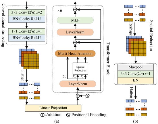
Figure 2.
The architecture of the CT encoder. (a) CT encoder; (b) spatial reduction operator.
After the convolution embedding, six transformer blocks as shown in Figure 2a are used to learn the global dependencies in the image. First, feature maps from the convolution embedding block are flattened and projected as embedded features with the position information. In the transformer block, the linear projection is first added with position information and then fed into the layer normalization (LayerNorm) [42]. The LayerNorm can be written as:
where is the linear projection containing position encoding. and denote gain and bias, respectively. and are the mean and variance of the elements in . is small and is introduced to avoid meaningless computation. Then, the output of the LayerNorm is viewed as , , and . Obviously, , , and are the same and are used for the calculation of self-attention. Furthermore, residual connections are added for effective learning.
Moreover, to reduce the computation cost for feature maps with large sizes, the multi-head attention with spatial reduction (SRA) [43] is considered to model the representations of the LRMS and PAN images in different subspaces. In Figure 2a, and are first fed into SRA to reduce their size, specifically the number of rows in and . Then, and the outputs of SRA are regarded as the inputs of the multi-head attention module to calculate the attention among them. Thus, SRA is introduced into Figure 2a for less computation cost, and the SRA operator is shown in Figure 2b. By SR of the ith CT encoder, we reduce the sizes of key and value via the SR operator :
where is the down-sampling ratio in the SR operator of the ith CT encoder. The convolution layer in Equations (2) and (3) involves filters with the size of . and are the corresponding linear projection matrices. reshapes or to their 3D counterparts. denotes flattening, which is also the inverse operation of . For the three cascaded CT encoders in sub-networks, we set the down-sampling ratio set as 4, 2, and 1. Through the settings, the sizes of feature maps at different scales will be the same.
When we obtain the reduced versions of and , according to the calculation of the attention mechanism in [43], SRA in the ith CT encoder can be calculated by:
where , , and are the linear projections of the jth head in the ith CT encoders. is the linear projection matrix for concatenated heads. T denotes the matrix transpose. is typically set as . is the number of heads in SRA and is set as 8. Finally, these features flow into a multi-layer perception (MLP). In the CT encoder, the local and global information in LR MS and PAN images can be described efficiently, which is helpful for the spatial and spectral preservation of the fused image.
2.2. Spatial–Spectral Interaction Attention Module
In MSIT, the feature maps are extracted from PAN and LR MS images through sub-networks. For existing DNN-based methods, there is no explicit attention mechanism to guarantee the interaction between sub-networks. Thus, it will lead to some redundant information among these features. To fuse the spatial and spectral features efficiently, we design a new attention module SIAM, which is shown in Figure 3. In SIAM, the feature maps and at the ith scale of sub-networks are unfolded firstly. The kernel size of the unfolding operator is with a stride of 4 in the first two CT encoders. For the last CT encoder, we set the kernel size of the unfolding operator as . Then, their corresponding key and value of are obtained by the linear projection and layer normalization:
where stands for the unfolding operator. and are the corresponding results after the linear projection of and , respectively. Similarly, through the linear projection matrices and , we produce the key and value of from the sub-network of the LR MS image. For the Query , it is estimated from the concatenation of and by:
where the concatenation operation is denoted by . is the linear projection matrix of . Then, the spatial–spectral interaction between sub-networks is achieved by:
where is equal to the number of columns of or . By the multiplication of and , the spatial information existing in is captured and encoded the attention result. In the same way, the spectral information is further highlighted by Equation (11). After the attention estimation with , the redundancy of these features is reduced and their complementarity is enhanced further. Finally, the features with interaction attention are folded and concatenated together for the generation of the fused image.
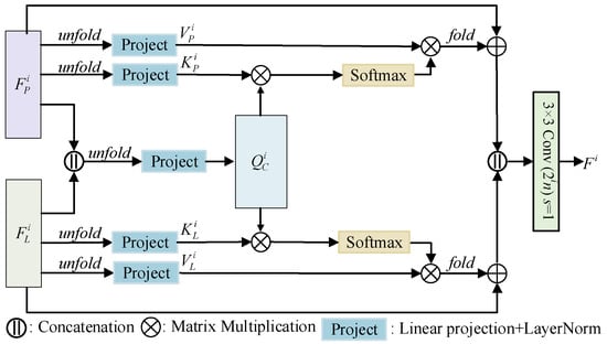
Figure 3.
The architecture of SIAM.
2.3. Multiscale Reconstruction Module
When the spatial and spectral features are fused by SIAMs at different scales, we propose an MRM to generate the desired HR MS image from these features. The architecture of MRM is presented in Figure 4. In MRM, the feature maps at coarse scales are up-sampled gradually via a block consisting of convolution and pixel shuffling [44]. In this block, pixel shuffling [44] is employed for the up-sampling of feature maps and the up-sampling ratio is 2 or 4, which is decided by the index of scale. The activation function used in MRM is LeakyReLU:
where is the element in feature maps and is a preset parameter. Before feature maps are fed into the pixel shuffling operator, the number of channels in the feature maps are improved by the previous convolution layer to enhance the spatial and spectral information. Compared with traditional up-sampling methods, pixel shuffling has a better reconstruction performance in the resolution improvement task. Then, the up-sampled feature maps are combined with those at fine scales to recover the spatial and spectral details in the HR MS image. Through the scale-wise fusion, the feature maps at fine scales are concatenated to produce the HR MS image.
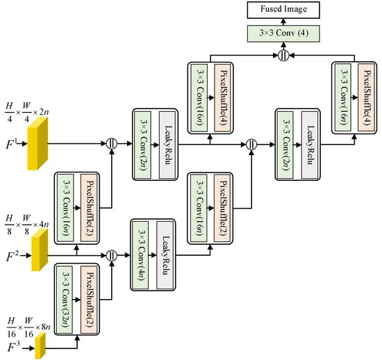
Figure 4.
The architecture of MRM.
2.4. Optimization
Finally, the proposed MSIT is learned by minimizing the loss:
where stands for the loss function. and are the reference image and the fused image, respectively. denotes the number of training images. Specifically, the proposed MSIT is trained on the PyTorch framework and the server is configured with an Intel Xeon 4210R/64G and an NVIDIA GeForce RTX 3080 GPU. The reliability and stability of Intel Xeon 4210R are better and the CPU is cost-effective. The GPU adopted in this paper behaves better in terms of parallel computing. Moreover, we use the Adam optimizer [45] to minimize the loss in Equation (13). The batch size is set as 4. The learning rate and the number of epochs are set as 0.0001 and 2000, respectively. When the proposed MSIT is trained, the LR MS and PAN images are fed into the model to produce the pan-sharpened MS image.
3. Experimental Results and Discussion
In this section, comparison experiments are conducted on the datasets from different satellites to verify the effectiveness of the proposed method. Then, ablation study and analysis of network structure are explored to present the proposed MSIT comprehensively. The source code is publicly available at https://github.com/RSMagneto/MSIT (accessed on 11 February 2022).
3.1. Dataset, Methods, and Metrics
In the experimental section, some classical methods and DNN-based methods are considered, including BDSD [7], SVT [46], VPLGC [47], A-PNN [31], DRPNN [34], PanNet [34], PSGAN [36], and TFNet [48]. BDSD and SVT are CS- and MRA-based methods, respectively. VPLGC is classified as a model-based method. The latter five methods are DNN-based methods. For DNN-based methods, they are trained and tested on the same server as that mentioned in Section 2.4. The codes of BDSD and A-PNN are downloaded from [49].
For a comprehensive comparison, the fusion experiments are conducted on the reduced-scale and full-scale datasets from GeoEye-1 [50] and QuickBird satellites [51]. In the reduced-scale case, the HR MS image named the reference image is available for reference-based evaluation. Thus, Wald’s protocol [52] is employed to produce the reduced-scale datasets. According to Wald’s protocol, the MS and PAN images at the original scale are first blurred and down-sampled by a specific ratio to synthesize the LR MS and PAN images. Generally, the down-sampling ratio is 4. Then, the original MS image is viewed as the reference image. Thus, the fused image obtained from the synthesized LR MS and PAN images is compared with the reference image directly. In the full-scale case, the reference image is unavailable. For no-reference evaluation, the fused image is compared with LR MS and PAN image from spectral and spatial perspectives, respectively.
Moreover, reduced-scale datasets are constructed for the training and test of the proposed MSIT and DNN-based methods. The GeoEye-1 dataset is made up of 700 image pairs. The sizes of LR MS and PAN images are and , respectively. These images are captured from Hobart, Australia in February 2009. In the QuickBird dataset, there are 600 image pairs and the sizes of LR MS and PAN images are the same as those of the GeoEye-1 dataset. The images in the QuickBird dataset are taken in September 2008 from Xi’an, China. Finally, the GeoEye-1 and QuickBird datasets are partitioned into for training, validation, and test. Furthermore, DNN-based methods are trained on the GeoEye-1 and QuickBird datasets independently to produce the best fusion results on the respective datasets. Table 1 presents the details of the used images from GeoEye-1 and QuickBird satellites.

Table 1.
Details of datasets from GeoEye-1 and QuickBird satellites.
For the reduced-scale experiments, the reference-based evaluation is achieved by three metrics, such as Q4 [53], spectral angle mapper (SAM) [54], and Erreur Relative Globale Adimensionnelle de Synthèse (ERGAS) [52]. Q4 and SAM are proposed to measure the spectral distortions in the fused image. Q4 varies from 0 to 1 and its best value Q4 is 1. For SAM, a smaller value means better fusion quality and the optimal value is 0. As a global metric, ERGAS records the spatial and spectral distortions of the fused image. Smaller ERGAS denotes the better result. In addition, Q4 and ERGAS are dimensionless and the measurement unit of SAM is ° and labeled in the following tables. In the full-scale experiments, we utilize , , and QNR [55] for the assessment of the fused images. The spatial and spectral information in the fusion result is measured by and , respectively. QNR is calculated by integrating and . For QNR, the value closer to 1 corresponds to the better fusion result. The metrics for full-scale evaluation are dimensionless.
3.2. Experiments on Reduced-Scale Dataset
In this section, the fusion experiments are performed on the reduced-scale GeoEye-1 and QuickBird datasets. For the intuitive perception, some interesting areas are highlighted by a red rectangle, and their magnified versions are placed in the bottom right corner of the fused image. Figure 5 shows the results of all compared methods on the GeoEye-1 dataset. Red, Green, and Blue bands in the fused images are selected to form the true color images in Figure 5 for comparison. The absolute difference maps between fused images and the reference image are also displayed for further perception. The color bar is also shown in Figure 5 and used as the reference for the analysis of the reconstruction performance in the absolute difference maps. LR MS and PAN images are displayed in Figure 5a,b. The reference image is given in Figure 5c. Compared with the reference image, it can be observed that the result of BDSD in Figure 5d has a better performance in terms of spatial details. However, some spectral distortions also arise in Figure 5d. For example, the tree area in the lower-left corner of Figure 5d presents an unnatural color. For the result of VPLGC in Figure 5f, we can see some spatial artifacts in the magnified area. DRPNN also suffers from blurring effects because some edges and textures of buildings in Figure 5h are lost. For spectral information, the hue of the result of A-PNN in Figure 5g is slightly different from the reference image. The color of the PSGAN result in Figure 5j is darker than that of other results. Furthermore, we can find that the reconstruction errors of BDSD, SVT, VPLGC, and DRPNN are obvious. In the building areas, traditional methods, such as BDSD, SVT, and VPLGC, have larger reconstruction errors. Furthermore, DRPNN also has a poor performance in terms of the reconstruction performance in building areas. For other DNN-based methods, the reconstruction errors are small. The reconstruction performance of DNN-based methods is better than that of the traditional methods. Compared with PSGAN and TFNet, the proposed method achieves the best approximation because errors in the difference map of the proposed method are closer to 0.

Figure 5.
Visual analysis of the fused images from different methods on the GeoEye-1 dataset. (a) LR MS image; (b) PAN image; (c) reference image; (d) BDSD; (e) SVT; (f) VPLGC; (g) A-PNN; (h) DRPNN; (i) PanNet; (j) PSGAN; (k) TFNet; (l) MSIT.
Table 2 lists the objective evaluations of the average results on the test image pairs from the reduced-scale GeoEye-1 dataset. The best values are boldfaced. Thus, the values of the proposed are the best, which reflect better fidelity of the MSIT result in spatial and spectral preservation. Furthermore, one can find that the metric values of A-PNN are close to those of the proposed MSIT.
Table 2.
Numerical evaluations of the fused images in Figure 5 (GeoEye-1 dataset).
The fusion results of different methods are presented in Figure 6. The fusion results in Figure 6 are composed of red, green, and blue bands in the corresponding fused images. The second and fourth rows in Figure 6 illustrate the absolute difference maps of all methods. The color bar in Figure 6 is the same as that in Figure 5. It is obvious that the color of the BDSD result in Figure 6d is distinct from that of the reference image. The SVT result in Figure 6e also contains spectral distortions, which may be caused by improper fusion of high frequencies in SVT. Similar to Figure 5g, the A-PNN result in Figure 6g has a different visual appearance in terms of hue. We can find some blurring effects in the results of VPLGC and DRPNN. The results of PanNet, PSGAN, TFNet, and MSIT have a competitive performance in terms of visual comparison. However, some spatial artifacts also can be observed from the result of TFNet in Figure 6k. The absolute difference maps in Figure 6 reflect similar performance. The errors of BDSD, VPLGC, and DRPNN are worse than those of other methods. The DNN-based methods can approximate the reference image better. However, their reconstruction performance is also limited in the edges of buildings. From the error maps, we can see that the proposed method behaves better in terms of reconstruction accuracy because more pixel values are closer to 0.
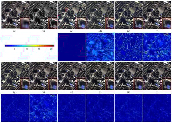
Figure 6.
Visual analysis of the fused images from different methods on the QuickBird dataset. (a) LR MS image; (b) PAN image; (c) reference image; (d) BDSD; (e) SVT; (f) VPLGC; (g) A-PNN; (h) DRPNN; (i) PanNet; (j) PSGAN; (k) TFNet; (l) MSIT.
Furthermore, we report the average performance of all methods on the 10% test dataset from the QuickBird satellite in Table 3. The best values in Table 3 are labeled in bold. The best values in Table 3 imply that the proposed MSIT is better than PanNet, PSGAN, and TFNet. For example, the ERGAS value of MSIT is much smaller than those of the compared methods.
Table 3.
Numerical evaluations of the fused images in Figure 6 (QuickBird dataset).
3.3. Experiments on Full-Scale Dataset
This section presents the fusion results of full-scale datasets from GeoEye-1 and QuickBird satellites. Figure 7 demonstrates the fusion results of all methods and the fusion results in Figure 7 are composited by red, green, and blue bands in the corresponding fused images. Compared with the LR MS image in Figure 7a, spatial details in the fused images of different methods are enhanced well. However, the spatial information is lost in the result of VPLGC in Figure 7e. For example, the magnified area in Figure 7e suffers from blurring effects, and the edges of the roof are blurred. The loss of spatial details in Figure 7e may be caused by the gradient constraint in VPLGC. For BDSD and TFNet, the spectral information in Figure 7c,j is not consistent with that of other fusion methods. For PanNet, PSGAN, and the proposed MSIT, visual differences can be found in the magnified areas of their results. The color of the PanNet result is over-enhanced. However, the spectral information in Figure 7i is distorted. The result of MSIT in Figure 7k has a better performance in terms of the spatial details. However, the color of the road areas in Figure 7k is slightly different from that in the original LR MS image of Figure 7a.
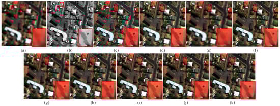
Figure 7.
Visual analysis of the fused images from different methods on the GeoEye-1 dataset. (a) LR MS image; (b) PAN image; (c) BDSD; (d) SVT; (e) VPLGC; (f) A-PNN; (g) DRPNN; (h) PanNet; (i) PSGAN; (j) TFNet; (k) MSIT.
The evaluation values of all test images from the full-scale GeoEye-1 dataset are provided in Table 4, where the best values are marked in bold. From Table 4, we can see that the proposed MSIT produces the best and , which means better preservation and enhancement in terms of spatial and spectral information. As an overall metric, the QNR of MSIT is also the best.
Table 4.
Numerical evaluations of the fused images in Figure 7 (GeoEye-1 dataset).
The fusion results on the full-scale QuickBird dataset are illustrated in Figure 8. The fusion results in Figure 8 are composed of the red, green, and blue bands of the fused images. We can see that the visual differences of different results are obvious. For instance, the spectral degradation is observed in the result of SVT in Figure 8d, and the color of the trees becomes gray. Compared with other methods, the local estimation of gains may lead to spatial distortions in the BDSD result, and the spatial information loss of VPLGC is the most serious. For DNN-based methods, obvious spectral distortions are generated in the roof and road areas of the PSGAN result in Figure 8i. For further perception, slight spectral loss appears in the magnified area of the TFNet result in Figure 8j. From the result of the proposed MSIT in Figure 8k, we can see that the color of the ground is nearly white when compared to the LR MS image in Figure 8a. Furthermore, some subtle texture information of tree areas is lost in Figure 8k when compared with the PAN image in Figure 8b. The loss of textural information makes it possible to separate the canopy from the trees.
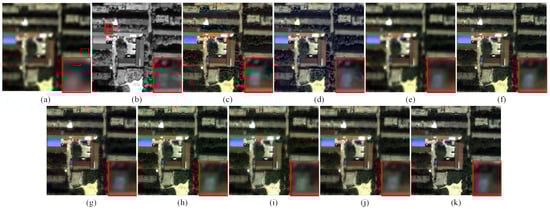
Figure 8.
Visual analysis of the fused images from different methods on the QuickBird dataset. (a) LR MS image; (b) PAN image; (c) BDSD; (d) SVT; (e) VPLGC; (f) A-PNN; (g) DRPNN; (h) PanNet; (i) PSGAN; (j) TFNet; (k) MSIT.
The 10% image pairs from the full-scale QuickBird dataset are randomly selected for the test, and Table 5 lists the average values of all metrics of the test image pairs. For the numerical results in Table 5, the best values are labeled in bold. The proposed MSIT provides the best values of all metrics, which demonstrate the effectiveness of SAIM in the proposed method.
Table 5.
Numerical evaluations of the fused images in Figure 8 (QuickBird dataset).
4. Discussion
In this section, the effects of the proposed MSIT are further discussed.
4.1. Ablation Study
The effectiveness of each module is verified by removing the module from the proposed MSIT in Figure 1. In Figure 9, we investigate the influences of the transformer block, SIAM, pixel shuffling, and MRM on the reduced-scale GeoEye-1 dataset. The absolute error maps between the reference image and the fused images are also displayed in the second row of Figure 9. Moreover, the third row of Figure 9 demonstrates the histograms of the reconstruction errors of different methods. Although it is difficult to distinguish the visual performance in Figure 9e,f, we can see obvious differences from the absolute error maps in Figure 9. More distortions in the texture areas result from the removal of the transformer block, which reflects the learning ability of the transformer block in terms of the global information. Furthermore, when MRM is removed, the errors are more obvious than those in other error maps. Thus, MRM can integrate spatial information at different scales efficiently. For the complete MSIT equipped with all modules, its fusion result shows the best reconstruction fidelity.
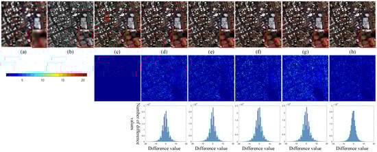
Figure 9.
Ablation study of different modules on the GeoEye-1 dataset. (a) LR MS image; (b) PAN image; (c) reference image; (d) w/o transformer block; (e) w/o SIAM; (f) w/o pixel shuffle; (g) w/o MRM; (h) complete MSIT.
The third row in Figure 9 shows the histograms of the difference values between the reference image and the fused images. The horizontal axis of the histogram represents the difference values. The number of difference values is reflected by the vertical axis of the histogram. There will be more difference values close to 0 if the reference image and the fused images are similar. From the histograms in the third row of Figure 9, we can see that most reconstruction errors for the results of different configurations are close to 0. For the complete MSIT, its variance in the histogram is smaller than that in other histograms. Smaller variance means that the reconstruction errors are closer to 0. Thus, the complete MSIT has better reconstruction performance when compared with other variants of MSIT. Table 6 provides objective evaluations of different fusion results in Figure 9. The best values are produced by the complete MSIT, which is consistent with the performance of error maps in Figure 9.
Table 6.
Numerical evaluations of the fused images in Figure 9 (GeoEye-1 dataset).
4.2. Comparison of Different Attention Modules
In this part, different attention mechanisms are explored to show the effectiveness of the proposed SIAM. Figure 10 illustrates two variants of SIAM. In Figure 10a, the attention mechanism is achieved by cascaded formulation. Thus, it is named a spatial–spectral cascaded attention module (SCAM). In Figure 10a, the spatial attention between the features of the PAN image and the concatenated image is estimated first. Then, spectral attention is calculated from the output of spatial attention and the LR MS image. Thus, the cascaded formulation will lead to the weakening of the spatial information in the extracted features because spatial attention is placed in front of spectral attention. Figure 10b plots the global attention mechanism, and it is dubbed as the spatial–spectral global attention module (SGAM). In the module, the concatenated image, PAN image, and LR MS image are regarded as query, key, and value to compute the global attention among these images. Then, feature maps with global attention are combined with PAN and LR MS images. In Figure 10b, the global attention ignores the differences between spatial and spectral features. Compared with the two variants in Figure 10, the adopted SIAM in Figure 3 estimates the spatial and spectral attention from PAN and LR MS images, respectively. Thus, the formulation of SIAM can ensure that as much spatial and spectral information as possible is learned efficiently.
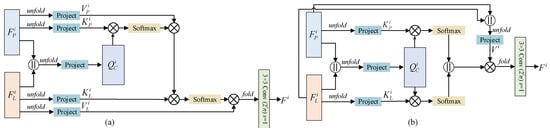
Figure 10.
Different variants of SIAM. (a) SCAM; (b) SGAM.
Figure 11 shows the fusion results of the proposed framework with different attention mechanisms on the reduced-scale GeoEye-1 dataset. The error maps and their corresponding histograms of the fused images are also given in the second and third rows of Figure 11. From Figure 11, we can see that the fusion results of SCAM and SGAM in Figure 11d,e suffer from spatial and spectral distortions. The phenomenon is obvious in the error maps. When SIAM in the proposed network is replaced by SCAM or SGAM, the reconstruction errors of the network become larger. Through the comparison of reconstruction errors in Figure 11, we can find that SIAM can extract the spatial and spectral features sufficiently in LR MS and PAN images.
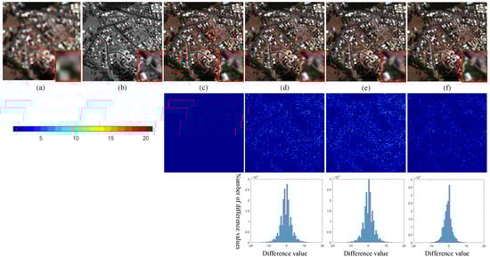
Figure 11.
Influences of different attention modules on the GeoEye-1 dataset. (a) LR MS image; (b) PAN image; (c) reference image; (d) SCAM; (e) SGAM; (f) SIAM.
The third row in Figure 11 demonstrates the histograms of the difference values between the reference image and the fused images. The horizontal axis and the vertical axis of the histogram record the difference values and the number of difference values, respectively. A larger number of values closer to 0 means better reconstruction performance. From the third row in Figure 11, it can be found that more reconstruction errors are concentrated near 0 in the histogram of SIAM compared with the other histograms of SCAM and SGAM. The numerical results of Figure 11 are demonstrated in Table 7, where the best values are labeled in bold. The improvement of Q4 and SAM is significant, which proves the effectiveness of the interaction attention mechanism.
Table 7.
Numerical evaluations of the fused images in Figure 11 (GeoEye-1 dataset).
4.3. Analysis of Network Architecture
In this part, we investigate the influences of the number of CT encoders on the fusion results. The LR MS and PAN images to be fused are from the reduced-scale GeoEye-1 dataset. With the introduction of more CT encoders into the proposed MSIT, the number of scales increases and the network is deeper. Concomitantly, the model size is larger. In this part, the number of CT encoders in the sub-networks varies from two to four. Fusion results of different architectures are shown in Figure 12. Moreover, the absolute error maps and histograms are also illustrated. We can find that the results in Figure 12d–f are close. However, as the network deepens, the errors in the second row of Figure 12 decrease first and then increase. The reconstruction errors of the network with three CT encoders are the smallest. For the network with two CT encoders, the representation capability may be limited by the depth of the network. Thus, the corresponding errors in Figure 12d are larger. When the sub-networks are composed of four4 CT encoders, the number of scales also increases and the size of feature maps in the fourth will be . The spatial and spectral information at coarse scales will be limited. Thus, CT encoders will extract more low-frequency information, which leads to inefficient training of the network. In the histograms of different network architectures, we can observe that the reconstruction errors are closer to 0 when the network is equipped with three CT encoders.
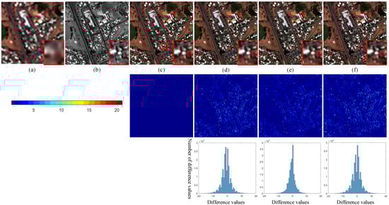
Figure 12.
Influences of different architectures on the GeoEye-1 dataset. (a) LR MS image; (b) PAN image; (c) reference image; (d) 2 CT encoders; (e) 3 CT encoders (MSIT); (f) 4 CT encoders.
Table 8 depicts the evaluation results of the fused images in Figure 12. The sub-networks with three CT encoders produce the best metric values in terms of Q4 and SAM. Furthermore, Table 8 also reports the training time and model size of the network with different CT encoders. Thus, more CT encoders mean a larger model size and more training time. Taking the overall performance of the proposed MSIT into consideration, we set the number of CT encoders in the proposed MSIT as three, finally.
Table 8.
Numerical evaluations of the fused images in Figure 12. (GeoEye-1 dataset).
4.4. Training and Test Time
To analyze the computation complexity, Table 9 gives the training and test times of all methods. Traditional methods need not be trained in advance, and thus only test time is recorded in Table 9. For DNN-based methods, although the structure of A-PNN is simple, satisfactory fusion results are achieved after enough iterations, e.g., iterations. For DRPNN and PanNet, the depth of the network is improved. Thus, the training time is more than that of A-PNN. PSGAN involves a more complex structure, which contains a generator and a discriminator. The complexity of PSGAN is higher than A-PNN, DRPNN, PanNet, and TFNet. For TFNet, the network is moderate. Thus, it can converge fast. Compared with other methods, the proposed MSIT needs more training time due to the involved matrix multiplication in the transformer block. For the test time, DRPNN and PSGAN spend more time. The test time of MSIT is comparable to that of TFNet.
Table 9.
Training and test times of different methods.
5. Conclusions
In this paper, we propose a new pan-sharpening method based on a multiscale spatial–spectral interaction transformer (MSIT). To capture the local and global properties in PAN and LR MS images, the sub-networks are constructed by a series of multiscale CT encoders for feature extraction. Then, SIAM is designed to integrate the features from the sub-networks. In SIAM, the interaction between the features from different sub-networks is achieved via the attention mechanism, which can enhance the complementarity and reduce the redundancy among spatial and spectral features. Finally, the spatial and spectral features at different scales are fed into MRM for the reconstruction of the fused image. In MRM, feature maps at coarse scales are up-sampled progressively to combine with the counterparts at fine scales. Through the architecture in MRM, the spatial and spectral information at different scales can be merged efficiently. The experiments at reduced and full-scale datasets from GeoEye-1 and QuickBird satellites demonstrate the effectiveness of the proposed MSIT in terms of objective and subjective evaluations. The multiscale transformer adopted in the proposed network can be easily used for the feature extraction of other related tasks, such as remote sensing image super-resolution. For future work, a transformer with more efficient structures will be explored to reduce the training and test time of the proposed method. Furthermore, the proposed method cannot efficiently preserve the spectral information in some areas containing rich color information, which may be caused by the information loss in MRM. Thus, we will also investigate more efficient reconstruction modules to integrate the spatial and spectral information in feature maps.
Author Contributions
Conceptualization, F.Z. and J.S.; Methodology, F.Z.; Software, F.Z.; Validation, K.Z.; Formal Analysis, F.Z.; Investigation, F.Z.; Resources, J.S.; Data Curation, K.Z.; Writing—Original Draft Preparation, F.Z.; Writing—Review and Editing, J.S.; Visualization, K.Z.; Supervision, J.S.; Project Administration, J.S.; Funding Acquisition, K.Z. and J.S. All authors have read and agreed to the published version of the manuscript.
Funding
This work was supported in part by the Natural Science Foundation of China (61901246), the China Postdoctoral Science Foundation Grant (2019TQ0190, 2019M662432), the Scientific Research Leader Studio of Jinan (2021GXRC081), and the Joint Project for Smart Computing of Shandong Natural Science Foundation (ZR2020LZH015).
Institutional Review Board Statement
Not applicable.
Informed Consent Statement
Not applicable.
Data Availability Statement
Not applicable.
Acknowledgments
The authors wish to acknowledge the three anonymous reviewers for providing helpful suggestions that greatly improved the manuscript.
Conflicts of Interest
The authors declare no conflict of interest.
References
- Baldinelli, G.; Bonafoni, S.; Rotili, A. Albedo Retrieval From Multispectral Landsat 8 Observation in Urban Environment: Algorithm Validation by in situ Measurements. IEEE J. Sel. Top. Appl. Earth Obs. Remote Sens. 2017, 10, 4504–4511. [Google Scholar] [CrossRef]
- Wang, M.; Hu, C. Automatic Extraction of Sargassum Features from Sentinel-2 MSI Images. IEEE Trans. Geosci. Remote Sens. 2021, 59, 2579–2597. [Google Scholar] [CrossRef]
- Vivone, G.; Mura, M.D.; Garzelli, A.; Restaino, R.; Scarpa, G.; Ulfarsson, M.O.; Alparone, L.; Chanussot, J. A new benchmark based on recent advances in multispectral pansharpening: Revisiting pansharpening with classical and emerging pansharpening methods. IEEE Geosci. Remote Sens. Mag. 2021, 9, 53–81. [Google Scholar] [CrossRef]
- Tu, T.-M.; Huang, P.S.; Hung, C.-L.; Chang, C.-P. A Fast Intensity–Hue–Saturation Fusion Technique With Spectral Adjustment for IKONOS Imagery. IEEE Geosci. Remote Sens. Lett. 2004, 1, 309–312. [Google Scholar] [CrossRef]
- Chavez, P., Jr.; Sides, S.C.; Anderson, J.A. Comparison of three different methods to merge multiresolution and multispectral data: Landsat TM and SPOT panchromatic. Photogramm. Eng. Remote Sens. 1991, 57, 295–303. [Google Scholar]
- Laben, C.A.; Brower, B.V. Process for Enhancing the Spatial Resolution of Multispectral Imagery Using Pan-Sharpening. U.S. Patent 6011875, 1 April 2000. [Google Scholar]
- Choi, J.; Yu, K.; Kim, Y. A new adaptive component-substitution-based satellite image fusion by using partial replacement. IEEE Trans. Geosci. Remote Sens. 2011, 49, 295–309. [Google Scholar] [CrossRef]
- Garzelli, A.; Nencini, F.; Capobianco, L. Optimal MMSE Pan Sharpening of Very High Resolution Multispectral Images. IEEE Trans. Geosci. Remote Sens. 2008, 46, 228–236. [Google Scholar] [CrossRef]
- Vivone, G. Robust Band-Dependent Spatial-Detail Approaches for Panchromatic Sharpening. IEEE Trans. Geosci. Remote Sens. 2019, 57, 6421–6432. [Google Scholar] [CrossRef]
- Aiazzi, B.; Baronti, S.; Selva, M. Improving component substitution pansharpening through multivariate regression of MS+Pan data. IEEE Trans. Geosci. Remote Sens. 2007, 45, 3230–3239. [Google Scholar] [CrossRef]
- Khan, M.M.; Chanussot, J.; Condat, L.; Montanvert, A. Indusion: Fusion of Multispectral and Panchromatic Images Using the Induction Scaling Technique. IEEE Geosci. Remote Sens. Lett. 2008, 5, 98–102. [Google Scholar] [CrossRef] [Green Version]
- Vivone, G.; Restaino, R.; Chanussot, J. Full Scale Regression-Based Injection Coefficients for Panchromatic Sharpening. IEEE Trans. Image Process. 2018, 27, 3418–3430. [Google Scholar] [CrossRef] [PubMed]
- Aiazzi, B.; Alparone, L.; Baronti, S.; Garzelli, A.; Selva, M. MTF-tailored Multiscale Fusion of High-resolution MS and Pan Imagery. Photogramm. Eng. Remote Sens. 2006, 72, 591–596. [Google Scholar] [CrossRef]
- Lee, J.; Lee, C. Fast and Efficient Panchromatic Sharpening. IEEE Trans. Geosci. Remote Sens. 2009, 48, 155–163. [Google Scholar]
- Shah, V.P.; Younan, N.H.; King, R.L. An Efficient Pan-Sharpening Method via a Combined Adaptive PCA Approach and Contourlets. IEEE Trans. Geosci. Remote Sens. 2008, 46, 1323–1335. [Google Scholar] [CrossRef]
- Shi, Y.; Yang, X.; Cheng, T. Pansharpening of multispectral images using the nonseparable framelet lifting transform with high vanishing moments. Inf. Fusion 2014, 20, 213–224. [Google Scholar] [CrossRef]
- Xing, Y.; Wang, M.; Yang, S.; Zhang, K. Pansharpening with Multiscale Geometric Support Tensor Machine. IEEE Trans. Geosci. Remote Sens. 2018, 56, 2503–2517. [Google Scholar] [CrossRef]
- Yin, H.; Li, S. Pansharpening with Multiscale Normalized Nonlocal Means Filter: A Two-Step Approach. IEEE Trans. Geosci. Remote Sens. 2015, 53, 5734–5745. [Google Scholar]
- Vivone, G.; Alparone, L.; Chanussot, J.; Mura, M.D.; Garzelli, A.; Licciardi, G.A.; Restaino, R.; Wald, L. A Critical Comparison among Pansharpening Algorithms. IEEE Trans. Geosci. Remote Sens. 2015, 53, 2565–2586. [Google Scholar] [CrossRef]
- He, X.; Condat, L.; Bioucas-Dias, J.; Chanussot, J.; Xia, J. A New Pansharpening Method Based on Spatial and Spectral Sparsity Priors. IEEE Trans. Image Process. 2014, 23, 4160–4174. [Google Scholar] [CrossRef] [PubMed]
- Zhang, K.; Wang, M.; Yang, S.; Xing, Y.; Qu, R. Fusion of Panchromatic and Multispectral Images via Coupled Sparse Non-Negative Matrix Factorization. IEEE J. Sel. Top. Appl. Earth Obs. Remote Sens. 2016, 9, 5740–5747. [Google Scholar] [CrossRef]
- Yang, S.; Zhang, K.; Wang, M. Learning Low-Rank Decomposition for Pan-Sharpening with Spatial-Spectral Offsets. IEEE Trans. Neural Networks Learn. Syst. 2017, 29, 3647–3657. [Google Scholar]
- Zhang, K.; Wang, M.; Yang, S.; Jiao, L. Convolution Structure Sparse Coding for Fusion of Panchromatic and Multispectral Images. IEEE Trans. Geosci. Remote Sens. 2018, 57, 1117–1130. [Google Scholar] [CrossRef]
- Palsson, F.; Sveinsson, J.R.; Ulfarsson, M. A New Pansharpening Algorithm Based on Total Variation. IEEE Geosci. Remote Sens. Lett. 2014, 11, 318–322. [Google Scholar] [CrossRef]
- Liu, P.; Xiao, L.; Zhang, J.; Naz, B. Spatial-Hessian-Feature-Guided Variational Model for Pan-Sharpening. IEEE Trans. Geosci. Remote Sens. 2015, 54, 2235–2254. [Google Scholar] [CrossRef]
- Liu, P.; Xiao, L. Multicomponent Driven Consistency Priors for Simultaneous Decomposition and Pansharpening. IEEE J. Sel. Top. Appl. Earth Obs. Remote Sens. 2019, 12, 4589–4605. [Google Scholar] [CrossRef]
- Ballester, C.; Caselles, V.; Igual, L.; Verdera, J.; Rougé, B. A Variational Model for P+XS Image Fusion. Int. J. Comput. Vis. 2006, 69, 43–58. [Google Scholar] [CrossRef]
- Dong, C.; Loy, C.C.; He, K.; Tang, X. Image Super-Resolution Using Deep Convolutional Networks. IEEE Trans. Pattern Anal. Mach. Intell. 2016, 38, 295–307. [Google Scholar] [CrossRef] [PubMed] [Green Version]
- Zhao, Z.-Q.; Zheng, P.; Xu, S.-T.; Wu, X. Object Detection with Deep Learning: A Review. IEEE Trans. Neural Netw. Learn. Syst. 2019, 30, 3212–3232. [Google Scholar] [CrossRef] [PubMed] [Green Version]
- Masi, G.; Cozzolino, D.; Verdoliva, L.; Scarpa, G. Pansharpening by Convolutional Neural Networks. Remote Sens. 2016, 8, 594. [Google Scholar] [CrossRef] [Green Version]
- Scarpa, G.; Vitale, S.; Cozzolino, D. Target-Adaptive CNN-Based Pansharpening. IEEE Trans. Geosci. Remote Sens. 2018, 56, 5443–5457. [Google Scholar] [CrossRef] [Green Version]
- He, K.; Zhang, X.; Ren, S.; Sun, J. Deep residual learning for image recognition. In Proceedings of the 2016 IEEE Conference on Computer Vision and Pattern Recognition (CVPR), Las Vegas, NV, USA, 27–30 June 2016. [Google Scholar]
- Yang, J.; Fu, X.; Hu, Y.; Huang, Y.; Ding, X.; Paisley, J. PanNet: A deep network architecture for pan-sharpening. In Proceedings of the IEEE International Conference on Computer Vision (ICCV), Venice, Italy, 22–29 October 2017; pp. 5449–5457. [Google Scholar]
- Wei, Y.; Yuan, Q.; Shen, H.; Zhang, L. Boosting the accuracy of multi-spectral image pan-sharpening by learning a deep residual network. IEEE Geosci. Remote Sens. Lett. 2017, 14, 1795–1799. [Google Scholar] [CrossRef] [Green Version]
- Goodfellow, I.J.; Pouget-Abadie, J.; Mirza, M.; Xu, B.; Warde-Farley, D.; Ozair, S.; Courville, A.; Bengio, Y. Generative adversarial nets. In Proceedings of the Neural Information Processing Systems (NIPS), Montreal, QC, Canada, 8–13 December 2014; pp. 2672–2680. [Google Scholar]
- Liu, Q.; Zhou, H.; Xu, Q.; Liu, X.; Wang, Y. PSGAN: A Generative Adversarial Network for Remote Sensing Image Pan-Sharpening. IEEE Trans. Geosci. Remote Sens. 2020, 59, 10227–10242. [Google Scholar] [CrossRef]
- Ma, J.; Yu, W.; Chen, C.; Liang, P.; Guo, X.; Jiang, J. Pan-GAN: An unsupervised pan-sharpening method for remote sensing image fusion. Inf. Fusion 2020, 62, 110–120. [Google Scholar] [CrossRef]
- Diao, W.; Zhang, F.; Sun, J.; Xing, Y.; Zhang, K.; Bruzzone, L. ZeRGAN: Zero-Reference GAN for Fusion of Multispectral and Panchromatic Images. IEEE Trans. Neural Networks Learn. Syst. 2022, 1–15. [Google Scholar] [CrossRef] [PubMed]
- Vaswani, A.; Shazeer, N.; Parmar, N.; Uszkoreit, J.; Jones, L.; Gomez, A.N.; Kaiser, L.; Polosukhin, I. Attention is all you need. In Proceedings of the Neural Information Processing Systems (NIPS), Long Beach, CA, USA, 4–9 December 2017; pp. 5998–6008. [Google Scholar]
- Yang, F.; Yang, H.; Fu, J.; Lu, H.; Guo, B. Learning texture transformer network for image super-resolution. In Proceedings of the IEEE Conference on Computer Vision and Pattern Recognition (CVPR), Virtual, 14–19 June 2020; pp. 5791–5800. [Google Scholar]
- Chen, H.; Wang, Y.; Guo, T.; Xu, C.; Deng, Y.; Liu, Z.; Ma, S.; Xu, C.; Xu, C.; Gao, W. Pretrained image processing transformer. In Proceedings of the IEEE Conference on Computer Vision and Pattern Recognition (CVPR), Virtual, 19–25 June 2021; pp. 1–10. [Google Scholar]
- Ba, J.; Kiros, J.; Hinton, G.E. Layer normalization. arXiv 2016, arXiv:1607.06450. [Google Scholar]
- Wang, W.; Xie, E.; Li, X.; Fan, D.; Song, K.; Liang, D.; Lu, T.; Luo, P.; Shao, L. Pyramid vision transformer: A versatile backbone for dense prediction without convolutions. In Proceedings of the IEEE International Conference on Computer Vision (ICCV), Virtual, 11–17 October 2021; pp. 568–578. [Google Scholar]
- Shi, W.; Caballero, J.; Huszár, F.; Totz, J.; Aitken, A.P.; Bishop, R.; Rueckert, D.; Wang, Z. Real-time single image and video super-resolution using an efficient sub-pixel convolutional neural network. In Proceedings of the IEEE Conference on Computer Vision and Pattern Recognition (CVPR), Las Vegas, NV, USA, 27–30 June 2016; pp. 1874–1883. [Google Scholar]
- Kingma, D.P.; Adam, J.B. A method for stochastic optimization. In Proceedings of the International Conference on Learning Representations (ICLR), San Diego, CA, USA, 7–9 May 2015; pp. 1–11. [Google Scholar]
- Zheng, S.; Shi, W.-Z.; Liu, J.; Tian, J. Remote sensing image fusion using multiscale mapped LS-SVM. IEEE Trans. Geosci. Remote Sens. 2008, 46, 1313–1322. [Google Scholar] [CrossRef]
- Fu, X.; Lin, Z.; Huang, Y.; Ding, X. A variational pan-sharpening with local gradient constraints. In Proceedings of the IEEE Conference on Computer Vision and Pattern Recognition (CVPR), Long Beach, CA, USA, 15–20 June 2019; pp. 10265–10274. [Google Scholar]
- Liu, X.; Liu, Q.; Wang, Y. Remote sensing image fusion based on two-stream fusion network. Inf. Fusion 2020, 55, 1–15. [Google Scholar] [CrossRef] [Green Version]
- Open Remote Sensing. Available online: https://openremotesensing.net/knowledgebase/a-new-benchmark-based-on-recent-advances-in-multispectral-pansharpening-revisiting-pansharpening-with-classical-and-emerging-pansharpening-methods/ (accessed on 18 March 2022).
- DigitalGlobe Product Samples. Available online: http://www.digitalglobe.com/product-samples (accessed on 16 March 2022).
- QuickBird. Available online: http://glcf.umiacs.umd.edu/data/quickbird/ (accessed on 20 June 2018).
- Wald, L.; Ranchin, T.; Mangolini, M. Fusion of satellite images of different spatial resolutions: Assessing the quality of resulting images. Photogramm. Eng. Remote Sens. 1997, 63, 691–699. [Google Scholar]
- Alparone, L.; Baronti, S.; Garzelli, A.; Nencini, F. A global quality measurement of pan-sharpened multispectral imagery. IEEE Geosci. Remote Sens. Lett. 2004, 1, 313–317. [Google Scholar] [CrossRef]
- Yuhas, R.H.; Goetz, A.; Boardman, J. Boardman. Discrimination among semi-arid landscape endmembers using the Spectral Angle Mapper (SAM) algorithm. In Proceedings of the Summaries 3rd Annual JPL Airborne Geoscience Workshop, Pasadena, CA, USA, 1 June 1992; pp. 147–149. [Google Scholar]
- Alparone, L.; Aiazzi, B.; Baronti, S.; Garzelli, A. Multispectral and panchromatic data fusion assessment without reference. Photogramm. Eng. Remote Sens. 2008, 74, 193–200. [Google Scholar] [CrossRef] [Green Version]
Publisher’s Note: MDPI stays neutral with regard to jurisdictional claims in published maps and institutional affiliations. |
© 2022 by the authors. Licensee MDPI, Basel, Switzerland. This article is an open access article distributed under the terms and conditions of the Creative Commons Attribution (CC BY) license (https://creativecommons.org/licenses/by/4.0/).