
Integrating UAV-SfM and Airborne Lidar Point Cloud Data to Plantation Forest Feature Extraction


Abstract

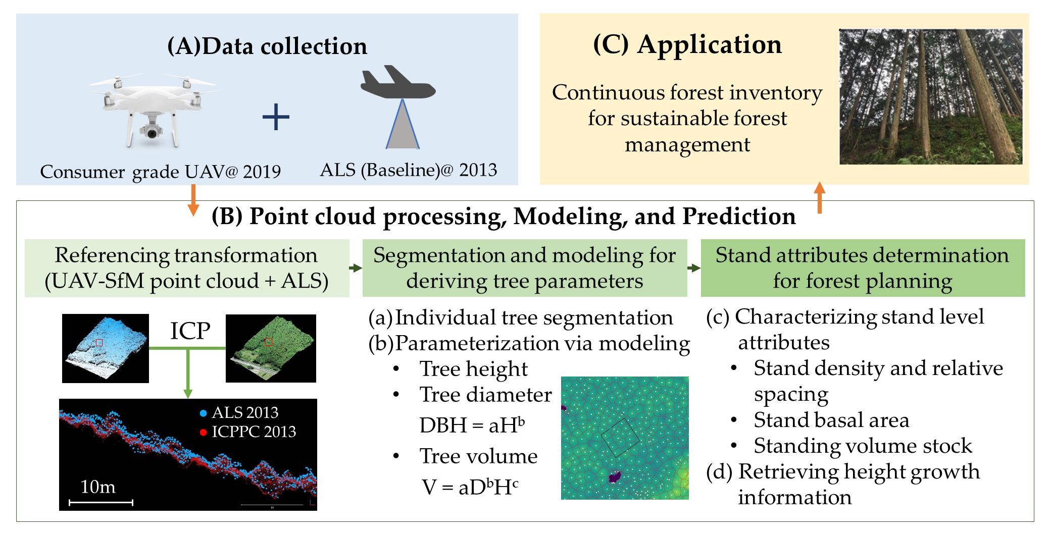
1. Introduction
2. Materials and Methods
2.1. Study Site
2.2. Airborne Lidar Data and UAV Data Collection and Processing
2.2.1. ALS Data
2.2.2. UAV Data
UAV-SfM Raw Point Cloud Generation
UAV-SfM and ALS Point Cloud Referencing Transformation
Bias-Adjustment by Invariant-Ground-Surface Altitude
UAV-SfM-Based Canopy Height Model Generation
2.3. Determination of Tree Volumetric Parameters for Both ALS and UAV Datasets
2.4. Deriving Annual Growth Rate of Tree Height
2.5. Assessment of Tree Height and Volume Models Performance
3. Results
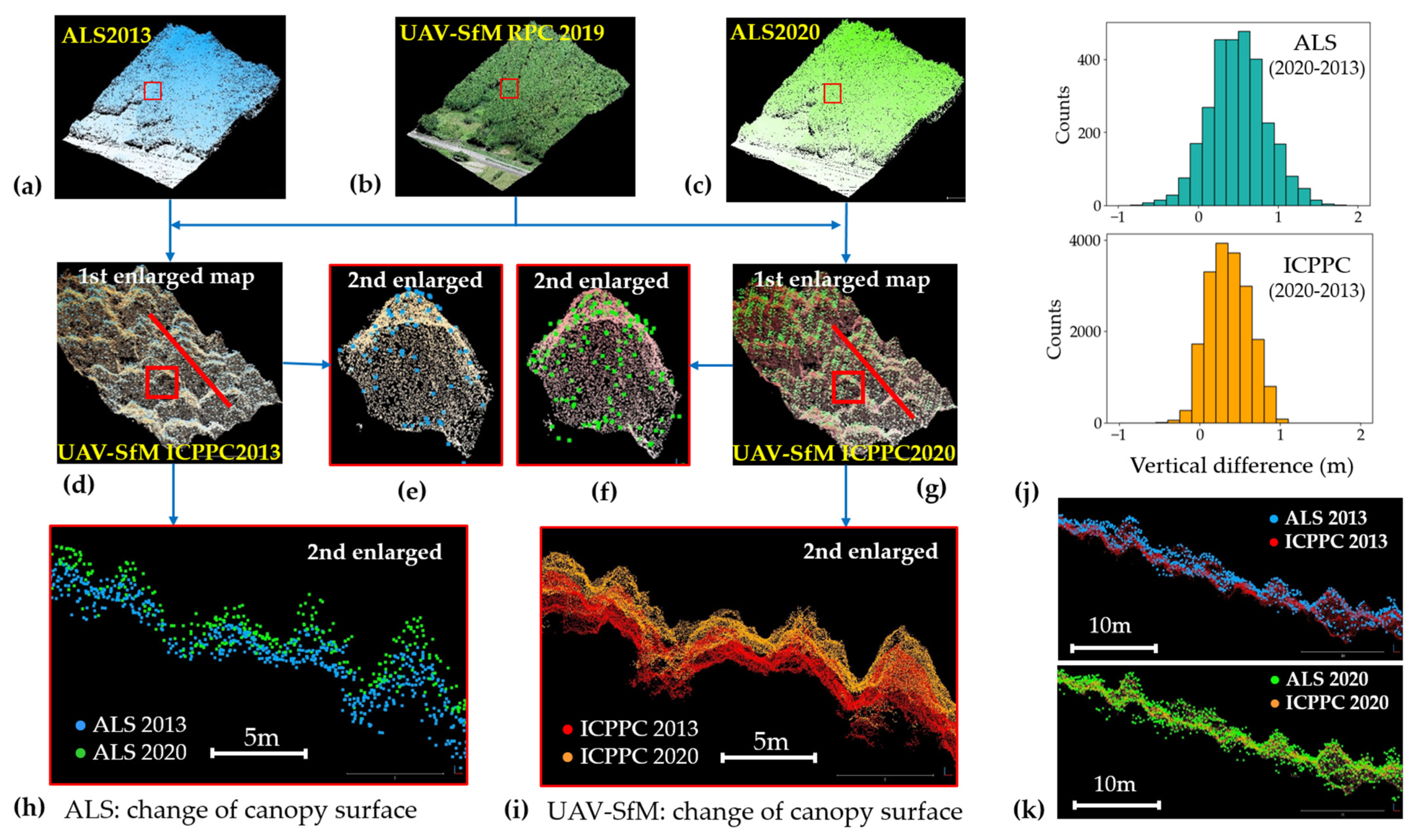
3.1. The Performance of the ICP and Bias-Adjustment Methods in Registering UAV-SfM Point Cloud Data to the ALS Point Cloud Model
3.2. Tree Segmentation Accuracy of CHM Data via the UAV-SfM and ALS-GM Approaches
3.3. Estimated Accuracy of Tree Volumetric Parameters of UAV-SfM and ALS-GM Approaches
3.3.1. Tree Height
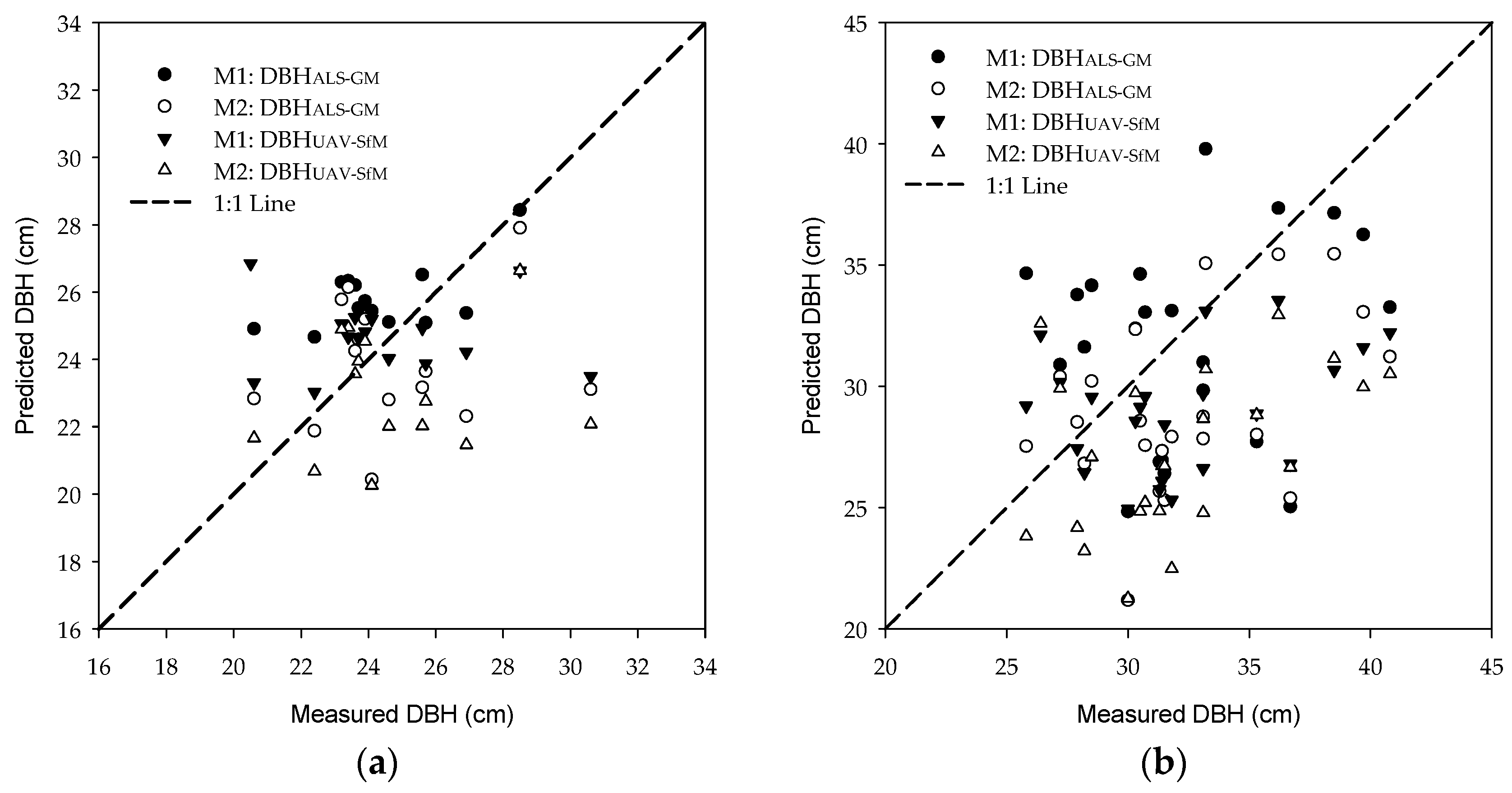
3.3.2. Tree Diameter
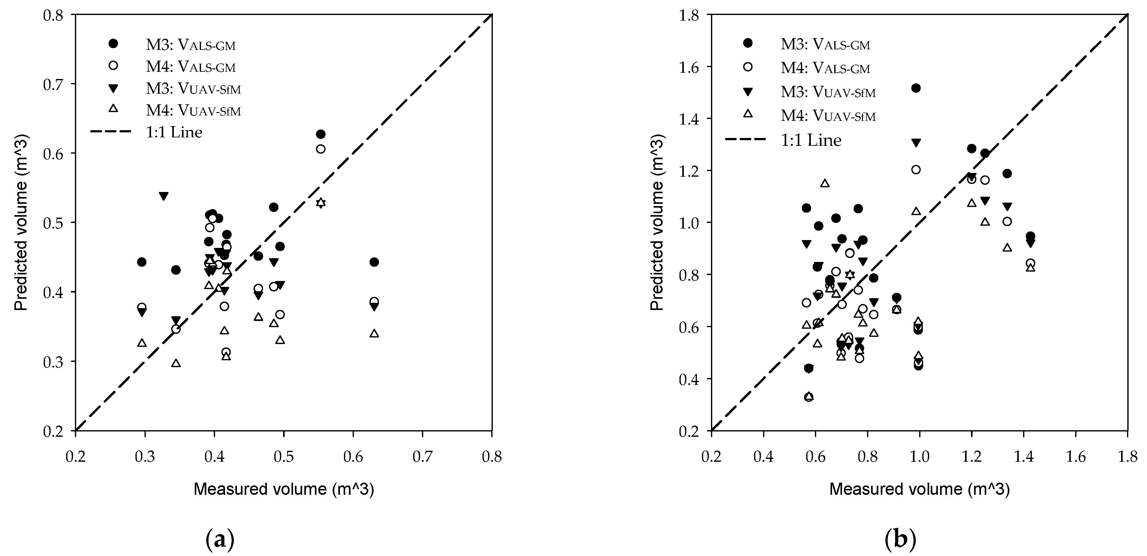
3.3.3. Tree Volume
4. Discussion
4.1. Performance of UAV-SfM Point Cloud Data in Characterizing Stand-Level Attributes
4.2. The Potential of Deriving Height Growth Information for Forest Monitoring via Integration of ALS and UAV-SfM Data
4.3. An Additional View on the Use of Enterprise-Grade UAV-Based Sensors for Forest Inventory
5. Conclusions
Author Contributions
Funding
Institutional Review Board Statement
Data Availability Statement
Acknowledgments
Conflicts of Interest
References
- Lin, C.; Thomson, G.; Hung, S.H.; Lin, Y.D. A GIS-based protocol for the simulation and evaluation of realistic 3-D thinning scenarios in recreational forest management. J. Environ. Manag. 2012, 113, 440–446. [Google Scholar] [CrossRef] [PubMed]
- Matsumura, N.; Yurugi, Y.; Numamoto, S. Philosophy and techniques for forest resource management: Follow up and new challenges for coming generations. J. For. Plan. 2013, 18, 91–98. [Google Scholar]
- Bowditch, E.; Santopuoli, G.; Binder, F.; del Rio, M.; Porta, N.L.; Kluvankova, T.; Lesinski, J.; Motta, R.; Pach, M.; Panzacchi, P.; et al. What is climate-smart forestry? A definition from a multinational collaborative process focused on mountain regions of Europe. Ecosyst. Serv. 2020, 43, 101113. [Google Scholar] [CrossRef]
- Sheremet, O.; Rulkamo, E.; Juutinen, A.; Svento, R.; Hanley, N. Incentivising participation and spatial coordination in payment for ecosystem service schemes: Forest disease control programs in Finland. Ecol. Econ. 2018, 152, 260–272. [Google Scholar] [CrossRef]
- Lin, C.; Tsogt, K.; Zandraabal, T. A decompositional stand structure analysis for exploring stand dynamics of multiple attributes of a mixed-species forest. For. Ecol. Manag. 2016, 378, 111–121. [Google Scholar] [CrossRef]
- Gil-Tena, A.; Saura, S.; Brotons, L. Effects of forest composition and structure on bird species richness in a Mediterranean context: Implications for forest ecosystem management. For. Ecol. Manag. 2007, 242, 470–476. [Google Scholar] [CrossRef]
- Holmgren, J.; Persson, Å. Identifying species of individual trees using airborne laser scanner. Remote Sens. Environ. 2004, 90, 415–423. [Google Scholar] [CrossRef]
- Lin, C.; Popescu, S.C.; Thomson, G.; Tsogt, K.; Chang, C.I. Classification of tree species in overstorey canopy of subtropical forest using QuickBird images. PLoS ONE 2015, 10, e0125554. [Google Scholar] [CrossRef]
- Lin, C.; Thomson, G.; Lo, C.S.; Yang, M.S. A multi-level morphological active contour algorithm for delineating tree crowns in mountainous forest. Photogramm. Eng. Remote Sens. 2011, 77, 241–249. [Google Scholar] [CrossRef]
- Bunting, P.; Lucas, R. The delineation of tree crowns in Australian mixed species forests using hyperspectral Compact Airborne Spectrographic Imager (CASI) data. Remote Sens. Environ. 2006, 101, 230–248. [Google Scholar] [CrossRef]
- Duncanson, L.I.; Cook, B.D.; Hurtt, G.C.; Dubayah, R.O. An efficient, multi-layered crown delineation algorithm for mapping individual tree structure across multiple ecosystems. Remote Sens. Environ. 2014, 154, 378–386. [Google Scholar] [CrossRef]
- Lo, C.S.; Lin, C. Growth-competition-based stem diameter and volume modeling for tree-level forest inventory using airborne LiDAR data. IEEE Trans. Geosci. Remote Sens. 2013, 51, 2216–2226. [Google Scholar] [CrossRef]
- Takahashi, T.; Yamamoto, K.; Senda, Y.; Tsuzuku, M. Estimating individual tree heights of sugi (Cryptomeria japonica D. Don) plantations in mountainous areas using small-footprint airborne LiDAR. J. For. Res. 2005, 10, 135–142. [Google Scholar] [CrossRef]
- Takahashi, T.; Yamamoto, K.; Senda, Y.; Tsuzuku, M. Predicting individual stem volumes of sugi (Cryptomeria japonica D. Don) plantations in mountainous areas using small-footprint airborne LiDAR. J. For. Res. 2005, 10, 305–312. [Google Scholar] [CrossRef]
- Lin, C.; Thomson, G.; Popescu, S.C. An IPCC-compliant technique for forest carbon stock assessment using airborne LiDAR-derived tree metrics and competition index. Remote Sens. 2016, 8, 528. [Google Scholar] [CrossRef]
- Dalponte, M.; Coomes, D.A. Tree-Centric Mapping of Forest Carbon Density from Airborne Laser Scanning and Hyperspectral Data. Methods Ecol. Evol. 2016, 7, 1236–1245. [Google Scholar] [CrossRef]
- Vepakomma, U.; St-Onge, B.; Kneeshaw, D. Spatially explicit characterization of boreal forest gap dynamics using multi-temporal lidar data. Remote Sens. Environ. 2008, 112, 2326–2340. [Google Scholar] [CrossRef]
- Hopkinson, C.; Chasmer, L.; Hall, R.J. The uncertainty in conifer plantation growth prediction from multi-temporal lidar datasets. Remote Sens. Environ. 2008, 112, 1168–1180. [Google Scholar] [CrossRef]
- Wang, L.; Gong, P.; Biging, G.S. Individual tree-crown delineation and treetop detection in high-spatial-resolution aerial imagery. Photogramm. Eng. Remote Sens. 2004, 70, 351–357. [Google Scholar] [CrossRef]
- Hyyppä, J.; Kelle, O.; Lehikoinen, M.; Inkinen, M. A segmentation-based method to retrieve stem volume estimates from 3-D tree height models produced by laser scanners. IEEE Trans. Geosci. Remote Sens. 2001, 39, 969–975. [Google Scholar] [CrossRef]
- Lin, C.Y.; Lin, C.; Chang, I.C. A multilevel slicing based coding method for tree detection. In Proceedings of the 2018 IEEE International Geoscience and Remote Sensing Symposium, Valencia, Spain, 22–27 July 2018; pp. 7524–7527. [Google Scholar] [CrossRef]
- Morsdorf, F.; Meier, E.; Kötz, B.; Itten, K.I.; Dobbertin, M.; Allgöwer, B. LIDAR-based geometric reconstruction of boreal type forest stands at single tree level for forest and wildland fire management. Remote Sens. Environ. 2004, 92, 353–362. [Google Scholar] [CrossRef]
- Lee, A.C.; Lucas, R.M. A LiDAR-derived canopy density model for tree stem and crown mapping in Australian forests. Remote Sens. Environ. 2007, 111, 493–518. [Google Scholar] [CrossRef]
- Wallace, L.; Lucieer, A.; Malenovský, Z.; Turner, D.; Vopěnka, P. Assessment of forest structure using two UAV techniques: A comparison of airborne laser scanning and structure from motion (SfM) point clouds. Forests 2016, 7, 62. [Google Scholar] [CrossRef]
- Lisein, J.; Pierrot-Deseilligny, M.; Bonnet, S.; Lejeune, P. A Photogrammetric workflow for the creation of a forest canopy height model from small unmanned aerial system imagery. Forests 2013, 4, 922–944. [Google Scholar] [CrossRef]
- Lin, C.; Lo, K.L.; Huang, P.L. A classification method of unmanned-aerial-systems-derived point cloud for generating a canopy height model of farm forest. In Proceedings of the 2016 IEEE International Geoscience and Remote Sensing Symposium, Beijing, China, 10–15 July 2016; pp. 740–743. [Google Scholar]
- Xu, Z.; Li, W.; Li, Y.; Shen, X.; Ruan, H. Estimation of secondary forest parameters by integrating image and point cloud-based metrics acquired from unmanned aerial vehicle. J. Appl. Remote Sens. 2019, 14, 022204. [Google Scholar] [CrossRef][Green Version]
- Donager, J.; Sankey, T.T.; Meador, A.J.S.; Sankey, J.B.; Springer, A. Integrating airborne and mobile lidar data with UAV photogrammetry for rapid assessment of changing forest snow depth and cover. Sci. Remote Sens. 2021, 4, 100029. [Google Scholar] [CrossRef]
- Ministry of Agriculture Forestry and Fisheries. Area of Artificial Afforestation. The 93rd Statistical Yearbook of Ministry of Agriculture, Forestry and Fisheries. Available online: https://www.maff.go.jp/e/data/stat/93th/index.html (accessed on 29 January 2021).
- Bair, L.S.; Alig, R.J. Regional Cost Information for Private Timberland Conversion and Management; General Technical Report PNW-GTR-684; Forest Service, USDA: Portland, OR, USA, 2006; 32p.
- Nasiri, V.; Darvishsefat, A.A.; Arefi, H.; Griess, V.C.; Sadeghi, S.M.M.; Borz, S.A. Modeling forest canopy cover: A synergistic use of Sentinel-2, aerial photogrammetry data, and machine learning. Remote Sens. 2022, 14, 1453. [Google Scholar] [CrossRef]
- Yao, H.; Qin, R.; Chen, X. Unmanned aerial vehicle for remote sensing applications—A review. Remote Sens. 2019, 11, 1443. [Google Scholar] [CrossRef]
- Yoshii, T.; Matsumura, N.; Lin, C. Integrating UAV and lidar data for retrieving tree volume of hinoki forest. In Proceedings of the IGARSS 2020—2020 IEEE International Geoscience and Remote Sensing Symposium, Waikoloa, HI, USA, 26 September–2 October 2020; pp. 4124–4127. [Google Scholar] [CrossRef]
- Kokusai Kogyo Corporation (KKC). Etumisankei Aerial Laser Surveying Report; The Etsumi Sankei Sabo Office, Chubu Regional Development Bureau, MLIT: Ibi-gun, Japan, 2014; 104p.
- Aero Asahi Corporation (AAC). Forest Information Infrastructure Development Report No. 2; The Reiwa 2nd Year Forest Information Utilization Promotion Project No. 001-1-2002; Forestry and Forest Management Division, Department of Agriculture Forestry and Fisheries Mie Prefecture: Tsu City, Japan, 2020; 68p.
- James, M.R.; Robson, S. Straightforward reconstruction of 3D surfaces and topography with a camera: Accuracy and geoscience application. J. Geophys. Res. Earth Surf. 2012, 117, F03017.2. [Google Scholar] [CrossRef]
- Besl, P.J.; McKay, N.D. A method for registration of 3-D shapes. IEEE Trans. Pattern Anal. Mach. Intell. 1992, 14, 239–256. [Google Scholar] [CrossRef]
- Westoby, M.J.; Brasington, J.; Glasser, N.F.; Hambrey, M.J.; Reynolds, J.M. “Structure-from-Motion” photogrammetry: A low-cost, effective tool for geoscience applications. Geomorphology 2012, 179, 300–314. [Google Scholar] [CrossRef]
- Lowe, D.G. Distinctive image features from scale-invariant keypoints. Int. J. Comput. Vis. 2004, 60, 91–110. [Google Scholar] [CrossRef]
- Snavely, N.; Seitz, S.M.; Szeliski, R. Modeling the World from Internet Photo Collections. Int. J. Comput. Vis. 2008, 80, 189–210. [Google Scholar] [CrossRef]
- Zörner, J.; Dymond, J.R.; Shepherd, J.D.; Wiser, S.K.; Jolly, B. LiDAR-based regional inventory of tall trees-Wellington, New Zealand. Forests 2018, 9, 702. [Google Scholar] [CrossRef]
- Shimada, H. Construction of yield tables for sugi (Cryptomeria japonica) and hinoki (Chamaecyparis obtusa) plantations applied to long-rotation management in Mie Prefecture. Bull. Mie Prefect. For. Res. Inst. 2010, 2, 1–28. [Google Scholar]
- Shimada, H. Relationships among the diameter at breast height, tree height, and crown width in old plantations in Mie prefecture: Development of a tool for control of stand density for production of timber with large diameters. Bull. Mie Prefect. For. Res. Inst. 2011, 3, 19–26. [Google Scholar]
- Japan Forestry Agency. Table for Calculating Stem Volume from Diameter at Breast Height and Tree Height in Western Japan; Japan Forestry Agency: Tokyo, Japan, 1970.
- Nakajima, T.; Matsumoto, M.; Sasakawa, H.; Ishibashi, S.; Tatsuhara, S. Estimation of growth parameters using the local yield table construction system for planted forests throughout Japan. J. For. Plan. 2010, 15, 99–108. [Google Scholar] [CrossRef]
- Brede, B.; Calders, K.; Lau, A.; Raumonen, P.; Bartholomeus, H.M.; Herold, M.; Kooistra, L. Non-destructive tree volume estimation through quantitative structure modeling: Comparing UAV laser scanning with terrestrial LIDAR. Remote Sens. Environ. 2019, 233, 111355. [Google Scholar] [CrossRef]
- Lin, C. Improved derivation of forest stand canopy height structure using harmonized metrics of full-waveform data. Remote Sens. Environ. 2019, 235, 111436. [Google Scholar] [CrossRef]
- Bouvier, M.; Durrieu, S.; Fournier, R.A.; Renaud, J.P. Generalizing predictive models of forest inventory attributes using an area-based approach with airborne LiDAR data. Remote Sens. Environ. 2015, 156, 322–334. [Google Scholar] [CrossRef]
- Lin, C.; Trianingsih, D. Identifying forest ecosystem regions for agricultural use and conservation. Sci. Agric. 2016, 70, 62–70. [Google Scholar] [CrossRef]
- Nakajima, T.; Shiraishi, N.; Kanomata, H.; Matsumoto, M. A method to maximise forest profitability through optimal rotation period selection under various economic, site and silvicultural conditions. N. Z. J. For. Sci. 2017, 47, 4. [Google Scholar] [CrossRef]


| Site | In Situ Inventory Date | UAV Acquisition Date | Stand Age in 2019 | ALS Acquisition Date | Stand Age in 2013 |
|---|---|---|---|---|---|
| Kameyama | 26 July 2019 | 26 July 2019 | 46 | 24 November 2013 | 40 |
| Owase | 14 September 2018 | 14 September 2018 | 65 | 27 September 2013 | 60 |
| Site | Kameyama | Owase | ||||
|---|---|---|---|---|---|---|
| Parameter ¶ | DBH (cm) | H (m) | V (m3) | DBH (cm) | H (m) | V (m3) |
| Minimum | 20.50 | 17.30 | 0.2954 | 25.80 | 16.90 | 0.5651 |
| Maximum | 30.60 | 19.10 | 0.6303 | 40.80 | 24.10 | 1.4265 |
| Mean | 24.49 | 18.06 | 0.4287 | 32.09 | 21.04 | 0.8446 |
| Standard deviation | 2.61 | 0.53 | 0.0836 | 4.07 | 1.72 | 0.2464 |
| ALS | UAV−SfM | Bias | |||||||
|---|---|---|---|---|---|---|---|---|---|
| Point ID | x | y | z | x | y | z | xyz | xy | z |
| 1 | −117,575.54 | 336.32 | 215.89 | −117,575.75 | 336.64 | 215.82 | 0.3916 | 0.0710 | 0.2724 |
| 2 | −117,572.46 | 332.01 | 213.96 | −117,572.59 | 332.22 | 213.80 | 0.2987 | 0.1650 | 0.1760 |
| 3 | −117,600.53 | 315.30 | 217.48 | −117,600.68 | 315.74 | 217.49 | 0.4629 | 0.0140 | 0.3272 |
| 4 | −117,597.58 | 311.60 | 215.68 | −117,597.89 | 311.55 | 215.55 | 0.3386 | 0.1290 | 0.2214 |
| 5 | −117,570.15 | 329.72 | 214.23 | −117,570.26 | 329.91 | 214.20 | 0.2182 | 0.0260 | 0.1532 |
| 6 | −117,567.22 | 325.50 | 212.53 | −117,567.12 | 325.49 | 212.22 | 0.3267 | 0.3100 | 0.0730 |
| 7 | −117,595.74 | 309.10 | 215.77 | −117,595.82 | 309.12 | 215.61 | 0.1790 | 0.1590 | 0.0582 |
| 8 | −117,564.66 | 322.82 | 212.96 | −117,564.79 | 323.16 | 212.88 | 0.3699 | 0.0760 | 0.2560 |
| 9 | −117,561.67 | 318.90 | 211.24 | −117,561.55 | 318.78 | 210.91 | 0.3699 | 0.3290 | 0.1196 |
| 10 | −117,590.13 | 302.33 | 214.19 | −117,590.30 | 302.45 | 214.02 | 0.2668 | 0.1700 | 0.1454 |
| 11 | −117,586.45 | 298.53 | 212.35 | −117,586.59 | 298.15 | 212.09 | 0.4820 | 0.2610 | 0.2866 |
| 12 | −117,559.04 | 316.23 | 211.70 | −117,559.11 | 316.35 | 211.50 | 0.2412 | 0.2010 | 0.0943 |
| 13 | −117,555.71 | 311.90 | 209.19 | −117,556.08 | 312.04 | 209.49 | 0.5002 | 0.3000 | 0.2830 |
| 14 | −117,584.61 | 295.99 | 212.42 | −117,584.87 | 295.73 | 212.70 | 0.4651 | 0.2820 | 0.2615 |
| 15 | −117,580.90 | 291.07 | 210.96 | −117,581.07 | 291.48 | 210.73 | 0.4990 | 0.2270 | 0.3142 |
| 16 | −117,553.78 | 309.24 | 210.20 | −117,554.07 | 309.37 | 210.00 | 0.3765 | 0.2010 | 0.2251 |
| 17 | −117,550.79 | 305.16 | 207.53 | −117,550.63 | 305.30 | 208.01 | 0.5280 | 0.4830 | 0.1509 |
| 18 | −117,578.99 | 288.58 | 211.12 | −117,579.16 | 289.03 | 211.17 | 0.4828 | 0.0480 | 0.3397 |
| 19 | −117,576.14 | 284.80 | 209.35 | −117,576.01 | 284.66 | 209.19 | 0.2514 | 0.1600 | 0.1371 |
| 20 | −117,547.91 | 302.80 | 208.96 | −117,548.17 | 302.85 | 208.88 | 0.2825 | 0.0850 | 0.1905 |
| 21 | −117,544.94 | 298.68 | 206.99 | −117,545.17 | 298.63 | 206.74 | 0.3391 | 0.2460 | 0.1650 |
| 22 | −117,573.67 | 282.06 | 210.05 | −117,573.92 | 282.21 | 209.90 | 0.3236 | 0.1480 | 0.2035 |
| 23 | −117,543.53 | 295.77 | 207.21 | −117,543.40 | 296.21 | 207.14 | 0.4604 | 0.0730 | 0.3214 |
| 24 | −117,539.38 | 291.46 | 205.28 | −117,539.43 | 291.90 | 205.16 | 0.4622 | 0.1240 | 0.3149 |
| 25 | −117,564.57 | 271.27 | 206.19 | −117,564.61 | 271.25 | 206.34 | 0.1591 | 0.1540 | 0.0281 |
| 26 | −117,549.53 | 364.42 | 214.93 | −117,549.22 | 364.74 | 214.90 | 0.4464 | 0.0280 | 0.3150 |
| 27 | −117,546.41 | 360.27 | 213.18 | −117,546.22 | 360.39 | 212.90 | 0.3588 | 0.2790 | 0.1595 |
| 28 | −117,545.98 | 343.03 | 211.55 | −117,546.31 | 343.01 | 211.36 | 0.3847 | 0.1900 | 0.2365 |
| 29 | −117,610.64 | 243.15 | 208.09 | −117,610.46 | 243.47 | 208.09 | 0.3643 | 0.0010 | 0.2576 |
| 30 | −117,607.91 | 238.14 | 206.09 | −117,607.88 | 238.56 | 205.85 | 0.4822 | 0.2400 | 0.2957 |
| RMSE (m) | 0.3704 | 0.1727 | 0.2128 |
| Area | Method | Ntrees ¶ | Dtrees ¶ | OE% | EC% | Precision | Recall | F-Score |
|---|---|---|---|---|---|---|---|---|
| Kameyama | UAV | 99 | 100 | 1.0 | 2.0 | 0.99 | 0.98 | 0.99 |
| ALS | 84 | 20.2 | 5.0 | 0.79 | 0.94 | 0.86 | ||
| Owase | UAV | 110 | 137 | 5.5 | 30.0 | 0.92 | 0.68 | 0.79 |
| ALS | 138 | 9.0 | 34.5 | 0.86 | 0.62 | 0.72 |
| Site | Dataset | H Estimates Mean ± Std (m) | Estimation Error ¶ Range (m) | Estimation Error Mean ± Std (m) | RMSE (m) | PRMSE (%) |
|---|---|---|---|---|---|---|
| Kameyama | UAV-SfM | 18.07 ± 0.55 | −0.69–1.29 | 0.30 ± 0.31 | 0.43 | 2.40 |
| ALS-GM | 18.71 ± 0.56 | 0.13–2.21 | 0.65 ± 0.48 | 0.81 | 4.50 | |
| ALS2013 | 16.73 ± 0.50 | −1.89–0.09 | 1.34 ± 0.42 | 1.41 | 7.78 | |
| Owase | UAV-SfM | 20.25 ± 1.23 | −1.58–1.31 | 0.91 ± 0.40 | 0.99 | 4.73 |
| ALS-GM | 21.82 ± 2.10 | −1.64–3.91 | 1.45 ± 0.80 | 1.65 | 7.84 | |
| ALS2013 | 20.66 ± 1.99 | −2.61–2.73 | 1.14 ± 0.89 | 1.45 | 6.87 |
| Site | Dataset | DBH Equation | Range of Estimates (cm) | Mean ± Std (cm) | RMSE (cm) | PRMSE (%) |
|---|---|---|---|---|---|---|
| Kameyama | ALS-GM | M1: Equation (5) | 24.66–28.44 | 25.91 ± 1.08 | 2.57 | 10.47 |
| M2: Equation (6) | 20.43–30.75 | 24.32 ± 2.50 | 3.18 | 12.96 | ||
| UAV-SfM | M1: Equation (5) | 23.03–26.85 | 24.67 ± 1.05 | 2.32 | 9.48 | |
| M2: Equation (6) | 20.25–29.86 | 23.42 ± 2.43 | 3.27 | 13.36 | ||
| Owase | ALS-GM | M1: Equation (5) | 24.84–39.79 | 32.19 ± 4.30 | 5.86 | 18.25 |
| M2: Equation (6) | 21.18–37.49 | 29.44 ± 3.84 | 5.58 | 17.38 | ||
| UAV-SfM | M1: Equation (5) | 24.94–33.56 | 28.95 ± 2.46 | 3.84 | 11.95 | |
| M2: Equation (6) | 21.25–32.95 | 27.25 ± 3.25 | 4.73 | 14.75 |
| Site | Dataset | Volume Equation | Range of Estimates (m3) | Mean ± Std (m3) | RMSE (m3) | PRMSE (%) |
|---|---|---|---|---|---|---|
| Kameyama | ALS-GM | M3: Equations (5) and (7) | 0.4312–0.6271 | 0.4929 ± 0.0561 | 0.0940 | 21.92 |
| M4: Equations (6) and (7) | 0.3129–0.7172 | 0.4430 ± 0.1017 | 0.1117 | 26.05 | ||
| UAV-SfM | M3: Equations (5) and (7) | 0.3603–0.5394 | 0.4332 ± 0.0494 | 0.0777 | 18.11 | |
| M4: Equations (6) and (7) | 0.2956–0.6555 | 0.3975 ± 0.0921 | 0.1092 | 25.47 | ||
| Owase | ALS-GM | M3: Equations (5) and (7) | 0.4393–1.5162 | 0.9016 ± 0.3062 | 0.3406 | 40.33 |
| M4: Equations (6) and (7) | 0.3280–1.3533 | 0.7619 ± 0.2567 | 0.2849 | 33.73 | ||
| UAV-SfM | M3: Equations (5) and (7) | 0.4407–1.3105 | 0.8187 ± 0.2416 | 0.2280 | 26.99 | |
| M4: Equations (6) and (7) | 0.3290–1.1468 | 0.6953 ± 0.2089 | 0.2146 | 25.40 |
| Stand Parameter/Index | Kameyama Site | Owase Site | ||||||||
|---|---|---|---|---|---|---|---|---|---|---|
| Ground | UAV | E% ¶ | ALS | E% | Ground | UAV | E% | ALS | E% | |
| Stand density (N, tree/ha) | 1042 | 1042 | 0.00 | 903 | −13.34 | 943 | 943 | 0.00 | 943 | 0.00 |
| Average stem diameter (cm) | 24.49 | 24.67 | 0.73 | 25.91 | 5.80 | 32.09 | 29.00 | −9.63 | 32.19 | 0.31 |
| Average stem height (m) | 18.06 | 18.07 | 0.06 | 18.71 | 3.60 | 21.04 | 20.20 | −3.99 | 21.82 | 3.71 |
| Average stem volume (m3) | 0.43 | 0.43 | 1.05 | 0.49 | 14.98 | 0.84 | 0.82 | −3.07 | 0.90 | 6.75 |
| Volume per plot (m3) | 6.43 | 6.50 | 1.03 | 7.39 | 14.97 | 19.43 | 18.83 | −3.07 | 20.74 | 6.74 |
| Stand volume stock (m3/ha) | 446.59 | 451.21 | 1.03 | 513.43 | 14.97 | 796.17 | 771.72 | −3.07 | 849.82 | 6.74 |
| Stand basal area (m2/ha) | 49.61 | 49.87 | 0.52 | 55.02 | 0.91 | 77.47 | 62.49 | −19.34 | 78.09 | 0.80 |
| Sr (%) | 17.20 | 16.70 | −2.91 | 16.60 | −3.49 | 15.40 | 16.00 | 3.90 | 15.20 | −1.30 |
| Descriptive Statistics | Age Years) | ALS_HAGR (m/yr) | ALS_HAGR (%/yr) | UAV_HAGR (m/yr) | UAV_HAGR (%/yr) |
|---|---|---|---|---|---|
| Minimum | 37 | 0.06 | 0.36 | 0.09 | 0.81 |
| Maximum | 82 | 0.47 | 6.07 | 0.52 | 4.96 |
| Average | 57.38 | 0.30 | 2.59 | 0.31 | 2.66 |
| STD | 17.71 | 0.08 | 1.09 | 0.06 | 0.84 |
Publisher’s Note: MDPI stays neutral with regard to jurisdictional claims in published maps and institutional affiliations. |
© 2022 by the authors. Licensee MDPI, Basel, Switzerland. This article is an open access article distributed under the terms and conditions of the Creative Commons Attribution (CC BY) license (https://creativecommons.org/licenses/by/4.0/).
Share and Cite
Yoshii, T.; Matsumura, N.; Lin, C. Integrating UAV-SfM and Airborne Lidar Point Cloud Data to Plantation Forest Feature Extraction. Remote Sens. 2022, 14, 1713. https://doi.org/10.3390/rs14071713
Yoshii T, Matsumura N, Lin C. Integrating UAV-SfM and Airborne Lidar Point Cloud Data to Plantation Forest Feature Extraction. Remote Sensing. 2022; 14(7):1713. https://doi.org/10.3390/rs14071713
Chicago/Turabian StyleYoshii, Tatsuki, Naoto Matsumura, and Chinsu Lin. 2022. "Integrating UAV-SfM and Airborne Lidar Point Cloud Data to Plantation Forest Feature Extraction" Remote Sensing 14, no. 7: 1713. https://doi.org/10.3390/rs14071713
APA StyleYoshii, T., Matsumura, N., & Lin, C. (2022). Integrating UAV-SfM and Airborne Lidar Point Cloud Data to Plantation Forest Feature Extraction. Remote Sensing, 14(7), 1713. https://doi.org/10.3390/rs14071713