Abstract
Examining the characteristics of vegetation change and associated spatial patterns under different protection levels can provide a scientific basis for national park protection and management. Based on the dense time-series Landsat enhanced vegetation index (EVI) data between 1986 and 2020, we utilized the Wild Binary Segmentation (WBS) approach to detect spatial and temporal characteristics of abrupt, gradual, and total changes in Wuyishan National Park. The differences in vegetation change in three protection-level areas (strictly protected [Prots], generally protected [Prot], and non-protected [NP]) were examined, and the contributions to their spatial patterns were evaluated through Geodetector. The results showed the following: (1) The highest percentage of area without abrupt change was in Prots (39.89%), and the lowest percentage was in NP (17.44%). The percentage of abrupt change frequency (larger than three times) increased from 4.40% to 9.10% and 12.49% with the decreases in protection. The significance test showed that the difference in changed frequencies was not significant among these regions, but the interannual variation of abrupt change in Prots was significantly different from other areas. (2) The vegetation coverage of the Wuyishan National Park generally improved. The total EVI change (TEVI) showed that the positive percentage of Prots and Prot was 90.43% and 91.71%, respectively, slightly higher than that of NP (88.44%). However, the mean greenness change of NP was higher than that of Prots and Prot. (3) The park’s EVI spatial pattern in 1986 was the strongest factor determining the EVI spatial pattern in 2020; the explanatory power reduced as the protection level decreased. The explanation power (q value) of abrupt vegetation change was lower and increased as the protection level decreased. The interaction detection showed that EVI1986 and TEVI had the strongest explanatory powers, but the explanatory ability gradually weakened from 0.713 to 0.672 to 0.581 in Prots, Prot, and NP, respectively. This study provided a systematic analysis of vegetation changes and their impacts on spatial patterns.
1. Introduction
Recent studies have shown that land use (e.g., cropland and large-scale tree plantations in low-productive areas in China, and silvicultural practices in developed countries) is the dominant factor in global greening [1,2]. Protection measures (e.g., nature reserves, ecological functional zones) also provide an important basis for local vegetation greening [3]. Human exploitation and protection of land remain a complex and dynamic endeavor and have complex impacts on vegetation change and spatial patterns. China has carried out many conservation programs to promote vegetation restoration and mitigate climate change. However, the pressure on ecological environments has increased rapidly with the development of the economy and increasing human demand for natural resources in recent decades [4,5]. In these protected regions, the vegetation change was assumed to be increased greenness driven by natural factors, including natural growth and restoration and CO2 fertilization [6]. However, vegetation might degrade without human management, in advanced forest aging, and with climate change [7]. In the non-protected (NP) regions, vegetation change might be greening or browning, depending on its land use and cover. Evaluating the differences in vegetation changes in these complex zones (e.g., a national park and its peripheral areas) with human activities and protections can offer insights into their change mechanisms.
Temporal and spatial characteristics of vegetation changes have provided important information to assess the effectiveness of forest management and the potential of carbon sequestration [8]. Traditional vegetation dynamic detections were mainly based on remote sensing images from two or more dates using differencing and rating methods [9,10]. With the free availability of Landsat data in 2008 and the continuous improvement of time-series change detection technologies [11], the use of time-series data can clearly characterize the subtle changes and change processes of vegetation. Most of the current studies on vegetation change used trend analysis, correlation analysis, or other methods to analyze the spatial and temporal characteristics of vegetation change and the main driving factors. Some studies of time series Landsat data change detection characterized the forest disturbances and attributed the change agents [12]. However, few studies distinguished the different vegetation change processes (such as abrupt change and gradual change) and their different impacts on long-time greenness changes [1,5]. The vegetation change detection methods based on long time-series Landsat data can be grouped into three types: thresholding, segmentation, and model fitting [12]. The thresholding method mainly determines whether the pixel is a forest or not by setting the threshold value, and the time of exceeding the threshold value is treated as the change time [13]. The segmentation methods divide the long time-series remote sensing data into several segments and determine the location of abrupt changes according to the mean square error and other statistics [14,15]. These methods must determine the number of segments in advance. The model fitting fits a model using stable time-series data and calculates the difference between the predicted values of the fitted model and the observed values, and identifies the location of abrupt changes based on thresholds, least squares, etc. [16,17]. However, most of the current algorithms are subject to the selection of proper window sizes of the segments or model fitting, which are often difficult for detecting changes within small windows and near the starting and ending points. This leads to much uncertainty in vegetation change detection and trend analysis [3]. Recently, a random localization segmentation change detection method was proposed to locate the breakpoint with a flexible window [18]. It is capable of detecting the breakpoints in short intervals. However, this method has not been tested in time-series remote sensing data yet.
The difference in vegetation change between different protected levels has been widely investigated because it reveals the conservation effect of a natural reserve. The studies that used remote sensing data to quantify vegetation change in national parks can be grouped into (1) assessment of vegetation coverage based on multi-temporal remote sensing data and ecological index [19,20], and (2) a simple comparison before and after the establishment of the reserve and the difference in vegetation change in and outside the reserve to evaluate the conservation effectiveness [21,22,23]. The conclusions about the protective effects on vegetation coverage also showed differences: (1) Strictly protected (Prots) areas are more effective than NP areas [24,25]; (2) NP areas are more effective than Prots areas [26,27], which are exactly the opposite of (1); (3) There was no difference between the protected and NP areas [28,29]. However, most studies mainly focused on the overall trend of vegetation changes, and few studies have been conducted on the processes of vegetation change and their impacts on spatial patterns.
Understanding the major driving factors of spatial vegetation patterns at different protection levels plays a key role in ecological protection and is important for confronting climate change. The effects of different drivers on vegetation change were mainly explored by statistical methods such as regression analysis, correlation analysis, and residual methods [30,31,32]. These methods specialize in the analysis of the causes of time-series trends but mainly qualitatively describe their impacts on spatial patterns and fail to quantify the interactions among drivers. The geographical detector (Geodetector) can quantitatively study the spatial differentiation of geographic phenomena and their driving forces [33]. Its basic idea is assuming that the study area is divided into several subareas. It tests if the sum of the variance of subareas is less than the regional total variance; and if the spatial distribution of the two variables tends to be consistent. Geodetector can also determine whether there is an interaction effect between the two factors. This method was increasingly used to analyze the effects of natural factors (e.g., elevation, climate), anthropogenic factors (e.g., land use), and their interactions on vegetation growth spatial patterns [34]. However, most studies focused on the drivers of vegetation change, and very few studies have paid attention to the impacts of vegetation change processes on current vegetation coverage patterns [3].
In order to promote the scientific protection and rational utilization of natural resources and the harmonious coexistence between humans and nature, China proposed to establish nature reserves and ecological protection zones in the 1980s and national park systems in 2013 [35]. Wuyishan was selected as one of the first 10 pilot national parks in 2016 [36] and was identified as China’s first national park in 2021. Some regions of Wuyishan National Park had been strictly protected since the 1980s (e.g., the nature reserve), while some regions were set as ecological protection areas but still underwent human disturbances (e.g., tea plantations, scenic areas). Whether they experienced similar vegetation change processes and showed similar impacts on current spatial patterns was rarely investigated. We assume the spatial vegetation patterns were maximumly preserved in the Prots regions and significantly changed in the NP regions. However, such research is rarely seen in vegetation change analysis. Our study used the dense time series of Landsat enhanced vegetation index (EVI) data between 1986 and 2020 and a random localization segmentation method to reveal the spatial and temporal patterns of vegetation change at different protection levels in Wuyishan National Park and its peripheral areas using three indicators: abrupt, gradual, and total changes over the past 35 years. Specifically, we wanted to answer the following three questions through the analysis of vegetation change processes: (1) Do the abrupt vegetation changes show significant differences among different protection-level regions? (2) Are the vegetation browning and greening trends significantly different and do the protected regions show more obvious greening? (3) Which contributes more to the current vegetation spatial pattern: vegetation changes or initial vegetation coverage? A clear understanding of the vegetation changes and the driving factors of the current vegetation spatial patterns in Wuyishan National Park can provide a fundamental source for its protection, management, and sustainable development.
2. Materials and Methods
2.1. Study Area
Wuyishan National Park is located at the junction of Jiangxi and Fujian provinces in China (Figure 1). It includes Wuyishan National Nature Reserve in Fujian, Wuyishan Scenic Area, Jiuqu River Ecological Area, Wuyi Tianchi National Forest Park, and surrounding ecological forests, and part of Longhu Forest Farm of Shaowu City. The national park preserves the most complete, typical, and largest area of mesosubtropical native forest ecosystems of all that exist at the same latitude around the world [37]. The Fujian Wuyishan National Nature Reserve was established in 1979, and Wuyishan National Park was established in June 2016 and officially included as a national park in October 2021. Wuyishan National Park is adjacent to Wuyishan Nature Reserve in Jiangxi Province, which together form a complete, central subtropical forest ecosystem. The latter was established as a provincial nature reserve in 1981 and promoted to a national nature reserve in 2002. In this study, Wuyishan Nature Reserve in Fujian and Jiangxi provinces is categorized as a Prots area, the non-nature reserves within the national park are Prot areas, and a 5-km wide buffer zone around Wuyishan National Park is an NP area (Figure 1). The areas of Prots, Prot, and NP are 742.84 km2, 488.24 km2, and 1333.24 km2, respectively. Considering the NPs are in different counties, and the distances to urban centers (Figure 1a), population densities, intensities of human activities, and major vegetation types are very different, the NPs are divided into three subregions: NP in Guangze County (NPgz), NP in Yanshan County (NPys), and NP in Wuyishan City (NPwy). NPgz is dominated by broadleaf forests with some bamboo forests, mixed with Chinese fir and cropland; NPys is dominated by bamboo forests with some broadleaf forests, mixed with dispersed cropland; and NPwy is dominated by tea plantations and broadleaf forests with some bamboo forests and Chinese fir.
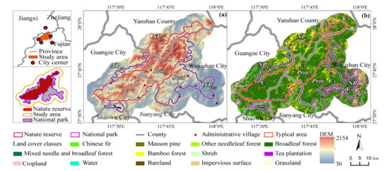
Figure 1.
Location of the study area. (a) is a digital elevation model; (b) shows land-cover types. Prots: Wuyishan Nature Reserve; Prot: non-nature reserve within the national park; NP: non-protected area; NPgz: non-protected area in Guangze County; NPys: non-protected area in Yanshan County; NPwy: non-protected area in Wuyishan City. C1, C2, C3, C4, and C5 are five study plots.
This region has a subtropical monsoon climate and elevation of 30~2154 m above sea level with obvious vertical vegetation zonality. The major vegetation types include evergreen broadleaf forest, needleleaf forest, needle-broadleaved mixed forest, bamboo forest, meadow, and tea plantation [38]. According to the regions with different protection levels and vegetation types, five 300 × 300 m typical plots were selected to show the vegetation change characteristics (Figure 1b). Plots C1 and C2 in Prots are dominated by broadleaf forest and bamboo forest, respectively. Plot C3 in Prot is dominated by Chinese fir with interspersed tea plantations. Plot C4 in NPys is mainly broadleaf forest, mixed with a few needleleaf forests and interspersed bamboo forests. Plot C5 in NPwy is predominantly impervious surface mixed with a few scattered barelands.
2.2. Data Preparation
We used Landsat L1T products (275 TM, 164 ETM+, and 89 OLI scenes) between April 1986 and October 2020 with cloud coverage of less than 80%, which were acquired from ESPA (https://espa.cr.usgs.gov/, accessed on 20 October 2020). These images were atmospherically calibrated [39]. Considering clouds, cloud shadows, and other noises, we further masked the low-quality pixels according to the quality bands [40,41]. These missing values in each time series EVI were labelled as NA values and were not involved in the change detection.
The imagery fused from the Gaofen-6 panchromatic band (2 m) and Sentinel-2 (10 m) by the Gram–Schmidt method in 2020 was used to develop land-cover data using a random forest classifier [42]. The land-cover classification system consists of 13 classes: Chinese fir forest, Masson pine forest, other needleleaf forest, broadleaf forest, mixed needle and broadleaf forest, bamboo forest, shrub, tea plantation, cropland, water, grassland, bareland, and impervious surface. A total of 785 samples were collected by field survey, and 70% of them were randomly selected as training samples, while 30% were taken as testing samples. The overall classification accuracy of 85% and a Kappa coefficient of 0.83 were obtained. The classification results were resampled to 30 m cell size using the nearest neighbor resampling method, resulting in the image in Figure 1b.
The terrain was chosen to analyze the impacts of vegetation changes on spatial patterns. ASTER GDEM was obtained from the geospatial data cloud platform with a spatial resolution of 30 m (https://www.gscloud.cn/, accessed on 20 Octobor 2020). The slope and aspect were extracted from the digital elevation model (DEM). All spatial data were clipped to the same extent as the study area.
2.3. Vegetation Change Detection Method
2.3.1. The Basic Principles of the Wild Binary Segmentation Method
The Wild Binary Segmentation (WBS) method, developed from Binary Segmentation (BS) and proposed by Fryzlewicz [18], has the advantage that it can detect changes that occurred in short time intervals and at the start and end periods of a time series. It does not need to preset the window size or span parameters and does not lead to a significant increase in computational complexity. WBS is sensitive to change points and can avoid the drawback of high omission in existing algorithms. The principle to find the change points is based on cumulative sum (CUSUM) (Equation (1)).
where s ≤ b < e, with n = e – s + 1; s and e are, respectively, the starting and ending points of the time series observations; b is the time (observation) between the starting and the ending points; Xt is the time-series value of a pixel at time t; and is the CUSUM statistic of b in the time series from s to e.
WBS starts by randomly segmenting time-series data into M (a large enough number to include all possible segmentations) segments, determines the breakpoint corresponding to the largest CUSUM value among all segments, and checks whether the breakpoint meets the criterion of the threshold or the strengthened Schwarz information. Once the first candidate breakpoint (b0) is determined, it divides all the time series that contain b0 into two segments ([s, b0] and [b0, e]). Then WBS finds the next candidate breakpoint by repeating the previous step. The maximum number of candidate breakpoints is predetermined, and the selected candidate breakpoints are recorded in descending order according to the CUSUM value. The order of the candidate breakpoints is an important indicator of the random segmentation process. A higher ranking has a higher probability that the breakpoint is real and represents a large abrupt change. WBS does not need to fit the model as other methods such as Breaks For Additive Seasonal and Trend (BFAST) [16], Landsat-based detection of Trends in Disturbance and Recovery (LandTrendr) [14], Continuous Change Detection and Classification (CCDC), and Continuous monitoring of Land Disturbance (COLD) [17] do. Thus, WBS has no strict requirements for the data length. Parameters setting in the WBS method mainly includes the following:
(1) Number of segmentations (M): Theoretically, M should be as large as possible to ensure that all possible segmentations can be included. A previous study showed that for time-series data whose number of observations does not exceed several thousand, setting M to 5000 can achieve excellent change detection [18]. WBS becomes standard BS when M is set to 0.
(2) Maximum number of breakpoints (k): k is the maximum change points that can be detected in the time-series data and can be set based on actual conditions and a priori experience.
(3) Criterion to confirm the breakpoints: Two criteria (thresholds [Equation (2)] and strengthened Schwartz Information Criterion [sSIC, Equation (3)]) can be used to confirm the detected breakpoints. If the CUSUM of the detected breakpoint exceeds the threshold, it will be confirmed as a candidate breakpoint. The sSIC does not need to set specific parameters, as it weighs the complexity of the estimated model and the goodness of the fitted data.
where is the threshold; T is the number of the time-series data; C is the default constant value; α corresponds to the SIC penalty; k: number of candidate breakpoints; is the corresponding maximum likelihood estimator of the residual variance.
2.3.2. Vegetation Change Detection and Accuracy Assessment
The WBS was used to detect the change points for the time-series EVI data of each pixel. Each time series was randomly segmented into M subsets (set to 5000), and CUSUMs were calculated to obtain the candidate change points. Fryzlewicz [18] argued that the parameter setting of the sSIC is simpler and more robust than the threshold method; thus, sSIC was chosen as the criterion for the breakpoint confirmation in our study. According to the field survey, the number of potential breakpoints in the study area was relatively low, so the maximum number of breakpoints (k) of each pixel was set to 8.
A total of 400 samples were randomly selected for assessing the change detection accuracies. They were manually interpreted using Google Earth [43]. Landsat images were used as reference data to determine whether and when the change occurred. Of the 400 samples, 250 samples experienced change, and 150 samples did not. The top ranking in the WBS results indicates a larger possibility of change in the time-series EVI when multiple breakpoints are detected for a pixel. The first two change times are then used, and the detected change time of the pixel is deemed to be correct as long as one of the detected change years is the same as the actual change year. The producer’s accuracy, user’s accuracy, and overall accuracy are used to assess the change detection results [44].
2.4. Analysis of Vegetation Change Characteristics
Vegetation change includes abrupt, gradual, and seasonal changes [45], and we focused on the first two types. A second-order harmonic model was used to fit the EVI of each pixel based on the detected breakpoints and the corresponding start and end times of each segment [45]. The fitted parameter of the trend was used to calculate the overall start and end values of the segment (Equation (4a,b)). The abrupt change at each breakpoint and gradual change of each segment were summed, respectively (AEVI in Equation (5) and GEVI in Equation (6)). We also summed the AEVI and GEVI as TEVI (Equation (7)). The AEVI represents the short-term change, or the change formed by the turning point of each vegetation change trend in the whole study period, such as rapid change induced by afforestation, fire, or deforestation and vegetation change from greening to browning. The GEVI refers to the change trend that occurred in the whole study period, such as vegetation growth or climate-induced vegetation change, reflecting the impacts of slowly acting environmental processes. TEVI indicates the net greening or net degradation of vegetation during the study period [3,46,47].
where and are the intercept and change trend (slope) for the ith segment; and are start and end times of the ith segment; and are calculated EVI at the start and end times of the ith segment based on the fitted parameters from the second-order harmonic model.
One-way ANOVA and a significance test were used to investigate whether the differences between regions were significant in changed times and annual changed area. The differences were grouped as extremely significant, significant, and not significant, according to the p values ≤ 0.01, ≤0.05, and >0.05, respectively. The changed area was standardized to 0–1 to make it comparable among different regions (Equation (8)), and the Tamhane method was used for the significance test [48].
where CA is the change area, CAmax is the maximum change area in each region, CAmin is the minimum changed area in each region.
2.5. Impact of Vegetation Changes on Spatial Patterns
Exploring the contribution of vegetation change processes to current spatial patterns is beneficial to understanding the driving mechanism. The factor detector and the interaction detector based on Geodetector were used to explore the explanatory powers of different factors on the current spatial patterns [33]. The mean EVI of the growing season in 1986–1988 (EVI1986) was calculated to represent the initial vegetation spatial pattern of the study area. The mean EVI of the growing season in 2019–2020 (EVI2020) was calculated to represent the current vegetation spatial pattern. EVI1986, DEM, Slope, Aspect, AEVI, GEVI, and TEVI were taken as independent variables, and EVI2020 was taken as the dependent variable to analyze the contribution of each factor to the current spatial pattern.
The factor detector was used to quantify the ability of each factor to explain the spatial heterogeneity of the current EVI spatial pattern. It is measured by q (Equation (9)); a larger q indicates the stronger explanation ability of the factor.
where h = 1, ..., L is the stratification of the independent variables; Nh and N are the number of cells in the hth stratum and the whole region, respectively; and are the variances of the hth stratum and the whole region, respectively; and SSW and SST are the sum of variance within the stratum and the sum within the whole region, respectively.
The interaction detector can identify the interactions between two factors and evaluate their explanations to the spatial heterogeneity of the current EVI spatial pattern. The interaction effects can be classified into enhanced, weak, or independent by comparing the recalculated q value with the previous q value (Table 1).

Table 1.
Criteria of interaction effects.
The Geodetector requires the independent factors to be categorical variables. The vegetation change factors (AEVI, GEVI, and TEVI) were divided into seven grades by quartiles and 0. EVI1986 and DEM were also divided into seven grades using the natural break method. The Slope and Aspect were categorized based on the grading standard in forestry surveys [49]. The specific groups are shown in Table 2.
Table 2.
Ranges of specific partitions of independent factors.
3. Results
3.1. Accuracy Assessment of Change Detection Results
The WBS showed very good performance in segmenting the whole time-series EVI into subsequences. The results of the change detection accuracy assessment showed an overall accuracy of 83% and changed samples had better accuracy than stable samples (Table 3). Considering the changed times, the overall accuracy was 60% for times matched to actual years and was 76% if a 1-year error was allowed. To further illustrate the process of vegetation change, Figure 2 shows the time-series EVI between 1986 and 2020 and the detected change points in typical plots. C1 shows broadleaf forests in Prots with an obvious negative abrupt change in 2007. The vegetation coverage gradually recovered and shifted to a degradation state in 2018. C2 illustrates bamboo forests in Prots with a stable-declined-stable-declined process. C3 shows Chinese fir in Prot with an obvious negative abrupt change in 1991. The stand gradually recovered and stabilized after 2000. C4 shows broadleaf forests in NPys and the time-series EVI divided into two relatively stable periods by a slightly positive abrupt change in 2007. C5 represents construction in NPwy with two obvious negative abrupt changes in 1998 and 2017. In the second change, the land-cover class changed to construction land.
Table 3.
Accuracy assessment of change detection results.
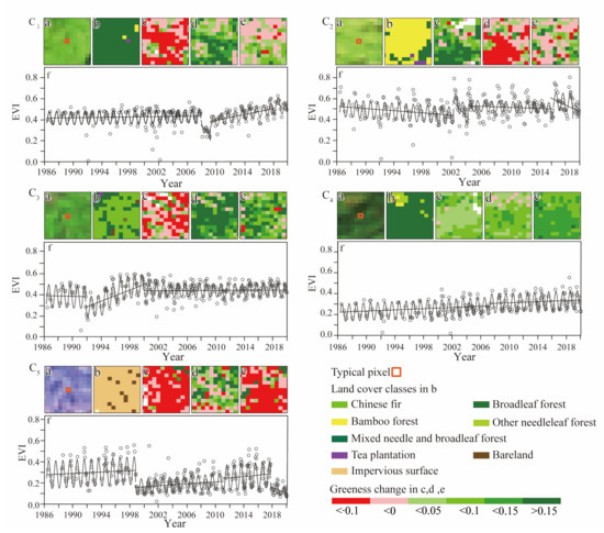
Figure 2.
Vegetation change characteristics and detected breakpoints in typical land-cover types. C1 and C2 are broadleaf forest and bamboo forest, respectively, in Wuyishan Nature Reserve; C3 is Chinese fir forest in Wuyishan National Park; C4 and C5 are broadleaf forest and construction land, respectively, in non-protected (NP) area. (a) Landsat OLI in 2020; (b) land-cover types in 2020; (c) cumulative abrupt change (AEVI); (d) cumulative gradual change (GEVI); (e) cumulative total change (TEVI); (f) time-series fitting curve of typical pixels (black dots are observations and lines are fitted by harmonic model).
3.2. Spatial and Temporal Characteristics of Abrupt Vegetation Change
As expected, protection measures have successfully decreased abrupt changes and change intensity. Prots had the highest percentage (39.89%) of detecting no breakpoints in the time-series EVI, and NP had the lowest percentage (17.44%). The percentages of the changed areas with more than three change points in Prots, Prot, and NP were 4.40%, 9.10%, and 12.49%, respectively (Figure 3). The differences in changed times were not significant among the three protection-level regions according to the significance test. Among the NP regions, the highest percentage of area without breakpoints was in NPys, and the lowest was in NPwy. NPgz and NPwy were also the main regions with more than three changed times (Figure 4).
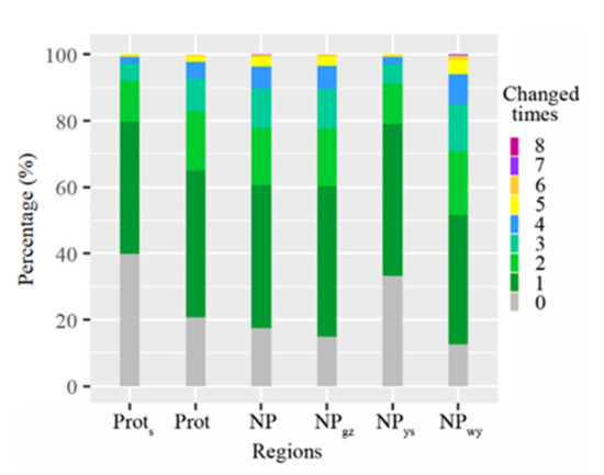
Figure 3.
Percentage of the changed times in different regions from 1986 to 2020. Prots: Wuyishan Nature Reserve; Prot: non-nature reserve within Wuyishan National Park; NP: non-protected area; NPgz: non-protected area in Guangze County; NPys: non-protected area in Yanshan County; NPwy: non-protected area in Wuyishan City.
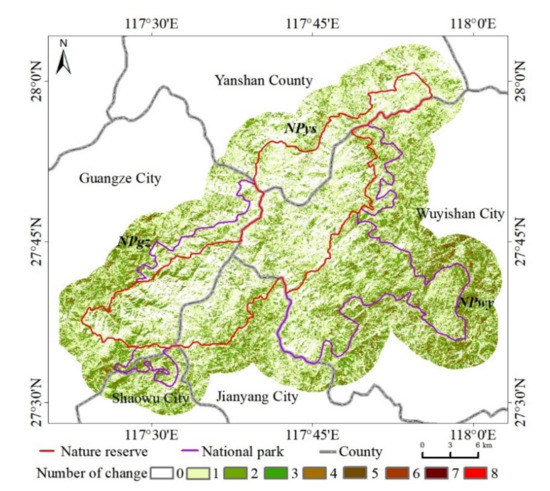
Figure 4.
The number of change times between 1986 and 2020 in the study area.
The annual changed areas showed a relatively consistent change trend among different regions between 1986 and 2020, except for some years with obvious differences (Figure 5). The annual abrupt change of Prots was extremely significantly different from that of all other regions, and Prot was significantly different from other regions except NPgz and NPwy (Table 4). The changed area increased significantly after 2003, with the largest changed areas occurring in Prots in 2004, Prot in 2016, and NP in 2016. The largest percentage of changed area in NPwy occurred the same year as in NP (2016), while large percentages of change occurred in both NPgz and NPys in 2009 (Figure 5). The differences between NPgz, NPys, and NP were extremely significant; the difference between NPwy and NP was not significant, indicating that NPwy dominated the change characteristics of NP (Table 4).
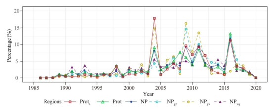
Figure 5.
The percentage of changed area between 1986 and 2020. Prots: Wuyishan Nature Reserve; Prot: non-nature reserve within Wuyishan National Park; NP: non-protected area; NPgz: non-protected area in Guangze County; NPys: non-protected area in Yanshan County; NPwy: non-protected area in Wuyishan City.
Table 4.
Significance test of the abrupt change area among different regions during 1986–2020.
3.3. Spatial and Temporal Patterns of Vegetation Brownness Change under Different Protection Levels
The percentage of negative vegetation change (AEVI, GEVI, and TEVI) in Prots was slightly lower than in Prot and NP, and so was the mean vegetation change (Table 5). This indicates that the vegetation coverage of Prots was relatively stable compared to other regions. The percentage of negative GEVI in each region was larger than that of AEVI except in NPwy. Both the mean and standard deviations of GEVI in NP (NPgz, NPys, and NPwy) were higher than that of Prots and Prot. The percentage of brown areas was smaller when considering AEVI and GEVI together (TEVI) than when AEVI and GEVI were calculated separately. The largest percentage of negative change among NP subregions occurred in NPwy. The mean vegetation changes in NPgz and NPys were significantly higher than in other regions.
Table 5.
The mean and negative percentages of abrupt, gradual, and total EVI changes.
The percentage of negative abrupt vegetation change each year had large variations among different regions, although they were all less than 20% between 1986 and 2020 (Figure 6). The highest percentages of negative abrupt change occurred in Prots and Prot with 15.7% and 14.8%, respectively, in 1998, and the highest percentages occurred in NP in 2007. The highest percentages occurred in NPwy, NPgz, and NPys in 1991 (10.3%), 2007 (16%), and 2007 (15.7%), respectively (Figure 6). The interannual variation of negative abrupt change area percentages in Prots, Prot, and NP were significantly different (Table 6). The difference in abrupt change area between NPgz and NPwy was not significant. However, the difference in negative vegetation change area between NPgz and NPwy was highly significant, because the negative abrupt change of NPwy was much higher than that of NPgz.
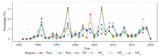
Figure 6.
The percentage of negative abrupt change area each year from 1986 to 2020. Prots: Wuyishan Nature Reserve; Prot: non-nature reserve within Wuyishan National Park; NP: non-protected areas; NPgz: non-protected areas in Guangze County; NPys: non-protected areas in Yanshan County; NPwy: non-protected areas in Wuyishan City.
Table 6.
Significance test of negative abrupt change area proportions among different regions during 1986–2020.
The negative AEVI and GEVI showed very different spatial patterns (Figure 7). The negative AEVI of Prots was mainly distributed in the broadleaf forests in the southwest region and near the villages in Prot. In NP, the negative AEVI was mainly distributed in the construction land in the NPwy subregion (Figure 7a). The negative GEVI of Prots was mainly distributed in the bamboo forests along the road and in scattered patterns in Prot and NP (Figure 7b). The GEVI of NP was higher than that of Prots and Prot, especially in the NPgz subregion. The significant vegetation degradation in NP was mainly distributed in the negative abrupt change areas in the NPwy subregion (Figure 7c).
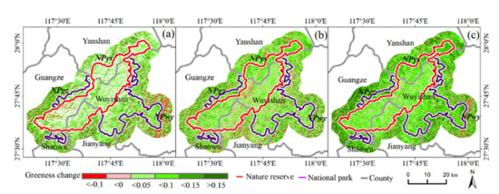
Figure 7.
EVI changes in the study area during 1986–2020. (a) abrupt EVI change (AEVI); (b) gradual EVI change (GEVI); (c) total EVI change (TEVI).
3.4. Contribution of Vegetation Changes to Current Spatial Patterns
EVI1986 had the strongest explanatory power of EVI2020 in three regions, but the explanatory power gradually reduced as the protection levels decreased (Table 7). Aspect also played a very important role in determining the current vegetation spatial patterns because of the complex topography in Wuyishan National Park. The explanatory power of AEVI and TEVI increased as the protection levels decreased. Among the three subregions of NP, the top two factors were still EVI1986 and aspect. The interaction results showed that the top explanatory powers were the interaction between EVI1986 and vegetation change processes (Appendix A Table A1), among which the interaction between EVI1986 and TEVI had the strongest explanatory power. TEVI reflected the total vegetation change characteristics during the study period, i.e., net greening or net degradation, and its interaction with EVI1986 together reflected the spatial characteristics of vegetation in 2020.
Table 7.
Factor detection in Wuyishan National Park during 1986–2020.
4. Discussion
4.1. Vegetation Change Characteristics of Wuyishan National Park
A large number of studies have been conducted to assess the ecological environment quality of Wuyishan Nature Reserve using different indicators such as remote sensing ecological index (RSEI) and fraction vegetation coverage (FVC) [5,50]. Their conclusions are consistent with our study, i.e., the vegetation coverage of Wuyishan Nature Reserve has been gradually improving in recent years. This study showed that the proportion of vegetation browning in protected areas (Prots and Prot) was significantly lower than in non-protected areas, which is consistent with Francçoso et al.’s results [51]. They used deforestation to assess the conservation effectiveness of protected areas in the Cerrado of Brazil and concluded that strictly protected areas have significantly lower deforestation than other areas. However, regions in non-protected areas also showed very low proportions of vegetation brownness, which was a benefit of land-use change and human management [2,52].
Although vegetation in Wuyishan National Park has generally shown positive change trends, some areas had degradation within the process of change. This is consistent with Li and Xiao’s analysis [53], which concluded that the ecological environment of the park was the worst in 2008. The broadleaf and bamboo forests at higher altitudes and on the northern slopes were seriously affected by the severe snowstorm in 2008 [54]. The bamboo forests along the road in Prots showed obvious degradation, and the invasion of bamboo seriously affected the vegetation in neighboring areas and showed a degradation trend [55]. The aging of bamboo forest might also make the vegetation turn brown because of the lack of harvesting and management. The most obvious degradation in Prot was attributed to the bamboo and Chinese fir forests near the villages, where the bamboo forests were degraded for the same reasons as in the Prots, and the Chinese fir forests were more likely to be affected by human disturbance and natural disasters. The most obvious degradation in NP was concentrated in NPwy, where rapid development of tourism and construction land has occurred in Wuyishan City. However, the average greenness of NP is higher than that of Prots, as the average greenness of NPgz and NPys was significantly higher than those of other areas. NPgz and NPys are lower in elevation than NPwy, thus are less affected by natural disasters such as landslides and mudslides from extreme climate conditions. They benefited from human management, and bamboo grows rapidly after the abrupt change of being selectively cut at a certain age [3]. Therefore, due to the influences of environmental characteristics and differences in management, the average vegetation greenness change in areas under strict protection is not always higher than that in non-protected areas, which is consistent with Li and Zhou’s results [56]. They concluded that the vegetation index of Wuyishan National Park increased due to many human activities and climate warming, while the increasing trend of vegetation index in scenic areas was significantly higher than that in protected areas. However, the increase in vegetation index was not equivalent to vegetation health, and the vulnerability was higher, and adaptability was lower in the scenic areas than those in protected areas [56].
Readers should keep in mind that most of the detected abrupt change showed positive change magnitude, which means later analyses of the segments yielded higher EVI than the earlier ones. Obviously, these abrupt changes, especially in Prots and Prot, were not driven by destructive disturbance events. One of the possible reasons is forest succession leads to very large changes in tree species composition. According to the investigation of a long-term observation of a forest sample plot in Prot, the dominant tree species changed from Castanopsis carlesii to Engelhardtia fenzlii Merr. from 2002 to 2015 [57]. The number of species and biodiversity decreased significantly; that is, about 26 tree species disappeared in the sample plot, and only six tree species newly emerged. Thus, a rapid forest succession might have an important impact on forest coverage and its change trend. Research also showed that there are significant differences in vegetation phenological characteristics in different regions under the dual influence of climate change and human activities [56]. Such impacts should be systematically evaluated in Wuyishan National Park. WBS is a statistical-based change detection method. Compared with Landtrendr, BFAST method, and so on, the major difference is its random localization segmentation mechanism and robustness to different lengths of time series. It can avoid the problem of a high omission rate for some areas where vegetation regrows rapidly after deforestation. However, the merit also means it is more sensitive to outliers, and there may be some pseudo change points were detected. Therefore, a more comprehensive assessment is necessary to validate and optimize the WBS method when applying it to time-series remote sensing data.
4.2. Influence of Different Drivers on the Current Spatial Characteristics of Vegetation in Wuyishan National Park
Extremely significant differences in the annual abrupt change in areas among Prots, Prot, and NP indicated that the change processes and influencing factors might vary in the three regions. Consistent with our assumption, the protection measures have contributed to preserving the initial vegetation coverage (in 1986) by reducing human activities, as that explanatory power was significantly larger in Prots. The vegetation change did not contribute much to the current spatial pattern of vegetation coverage, but the explanation power of vegetation changes also obviously increased with the decrease in protection levels. One of the important reasons is that vegetation change is more fragmented and has smaller values of change magnitudes compared with vegetation coverage values. Meanwhile, with the decrease in the degree of protection, the influence of human factors gradually increases, making spatial patterns of vegetation change more complex. This was also observed by Hartter et al. [58], who found that intact forests remain stable over time and fragmented areas are more prone to change. One important point is that AEVI had higher explanation power in protected regions, while TEVI showed higher explanation power in non-protected regions. This indicates that the vegetation change process was different in determining current spatial patterns. The explanatory power of aspect was ranked second among all factors, which indicates there was obvious spatial heterogeneity of vegetation cover because of the complex topography in Wuyishan National Park. The distribution of solar radiation in different aspects varies, and local natural factors such as precipitation and soil can also lead to differences in vegetation types and growth [59,60]. The interaction between EVI1986 and TEVI had the strongest explanatory power, which is consistent with Zhou et al.’s conclusion [61] that total change represented the vegetation change process better. In addition, AEVI showed higher explanatory power than GEVI in most regions when they interacted with EVI1986. This was different from the factor detection results and emphasized the necessity to distinguish the two change processes. However, the specific drivers (or events) of their dynamics need further analysis.
5. Conclusions
Dense time series of Landsat data between 1986 and 2020 were used to investigate the spatial and temporal patterns of vegetation change in Wuyishan National Park and peripheral areas at different protection levels. This study quantified the contributions of initial vegetation coverage and vegetation change processes to the current spatial patterns. The protection measures largely preserved the initial vegetation coverage in protected regions, but the vegetation greenness was lower than in non-protected regions. The initial vegetation spatial pattern (EVI1986) was the strongest factor determining the current EVI spatial pattern (EVI2020), no matter if an area was protected or not. However, the explanatory power gradually weakened as the protection levels decreased, and the explanatory power of vegetation change increased. The abrupt change frequency was not significantly different among regions, but the annual abrupt change areas had highly significant differences among Prots, Prot, and NP. Although most of the study areas experienced a greenness trend, some areas showed obvious vegetation brownness. The brownness distribution was different: the most significant vegetation degradation was mainly distributed in bamboo forests along the roads in Prots, more scattered and mainly near the villages in Prot, and in the construction land of NP. This study provided an important framework to evaluate vegetation change and its impact on spatial patterns at different protection levels, which is beneficial for future vegetation monitoring and national park management.
Author Contributions
Conceptualization, D.L. (Dengqiu Li) and D.L. (Dengsheng Lu); methodology, M.F., D.L. (Dengqiu Li), and D.L. (Dengsheng Lu); software, M.F.; validation, M.F., K.L., and D.L. (Dengqiu Li); formal analysis, M.F. and K.L.; investigation, M.F. and K.L.; resources, K.L., D.L. (Dengqiu Li), and D.L. (Dengsheng Lu); data curation, M.F. and D.L. (Dengqiu Li); writing—original draft preparation, M.F. and D.L. (Dengqiu Li); writing—review and editing, D.L. (Dengqiu Li) and D.L. (Dengsheng Lu); visualization, M.F. and D.L. (Dengsheng Lu); supervision, K.L., D.L. (Dengqiu Li), and D.L. (Dengsheng Lu); project administration, K.L., D.L. (Dengqiu Li), and D.L. (Dengsheng Lu); funding acquisition, K.L., D.L. (Dengqiu Li) and D.L. (Dengsheng Lu). All authors have read and agreed to the published version of the manuscript.
Funding
This research was funded by National Natural Science Foundation of China, grant number 41701490, National Key Research and Development Program of China, grant number 2016YFC0503302, and Fujian Provincial Science and Technology Department, grant number 2021R1002008).
Institutional Review Board Statement
Not applicable.
Informed Consent Statement
Not applicable.
Acknowledgments
The authors thank reviewers for their help to improve our manuscript.
Conflicts of Interest
The authors declare no conflict of interest.
Appendix A
Table A1.
Interaction detection in Wuyishan National Park during 1986–2020.
Table A1.
Interaction detection in Wuyishan National Park during 1986–2020.
| Prots | Prot | NP | NPgz | NPys | NPwy | ||||||
|---|---|---|---|---|---|---|---|---|---|---|---|
| Factor | q | Factor | q | Factor | q | Factor | q | Factor | q | Factor | q |
| EVI1986∩TEVI | 0.713 | EVI1986∩TEVI | 0.672 | EVI1986∩TEVI | 0.581 | EVI1986∩TEVI | 0.616 | EVI1986∩TEVI | 0.644 | EVI1986∩TEVI | 0.645 |
| EVI1986∩AEVI | 0.639 | EVI1986∩AEVI | 0.613 | EVI1986∩AEVI | 0.501 | EVI1986∩AEVI | 0.561 | EVI1986∩GEVI | 0.578 | EVI1986∩AEVI | 0.562 |
| EVI1986∩Aspect | 0.636 | EVI1986∩Aspect | 0.580 | EVI1986∩Aspect | 0.438 | EVI1986∩Aspect | 0.514 | EVI1986∩AEVI | 0.571 | EVI1986∩GEVI | 0.495 |
| EVI1986∩GEVI | 0.616 | EVI1986∩GEVI | 0.565 | EVI1986∩GEVI | 0.435 | EVI1986∩GEVI | 0.507 | EVI1986∩DEM | 0.565 | EVI1986∩Aspect | 0.487 |
| EVI1986∩DEM | 0.596 | EVI1986∩Slope | 0.545 | EVI1986∩Slope | 0.428 | EVI1986∩Slope | 0.506 | EVI1986∩Aspect | 0.561 | EVI1986 ∩Slope | 0.483 |
| EVI1986∩Slope | 0.585 | EVI1986∩DEM | 0.537 | EVI1986∩DEM | 0.419 | EVI1986∩DEM | 0.503 | EVI1986∩Slope | 0.517 | EVI1986∩DEM | 0.477 |
| Aspect∩TEVI | 0.421 | Slope∩Aspect | 0.348 | Aspect∩TEVI | 0.290 | Aspect∩TEVI | 0.311 | DEM∩Aspect | 0.365 | Aspect∩TEVI | 0.300 |
| DEM∩Aspect | 0.411 | DEM∩Aspect | 0.343 | Slope∩Aspect | 0.287 | Slope∩Aspect | 0.303 | Slope∩Aspect | 0.347 | Slope∩Aspect | 0.289 |
| Aspect∩AEVI | 0.400 | Aspect∩TEVI | 0.341 | DEM∩Aspect | 0.261 | DEM∩Aspect | 0.274 | Aspect∩TEVI | 0.333 | DEM∩Aspect | 0.274 |
| Slope∩Aspect | 0.399 | Aspect∩AEVI | 0.328 | Aspect∩AEVI | 0.240 | Aspect∩AEVI | 0.249 | Aspect∩AEVI | 0.308 | Aspect∩AEVI | 0.260 |
Note: The interaction factors were selected to rank the top 10; EVI1986: the initial enhanced vegetation index spatial pattern; AEVI: cumulative abrupt change; GEVI: cumulative gradual change; TEVI: cumulative total change; Prots: Wuyishan Nature Reserve; Prot: non-nature reserve within Wuyishan National Park; NP: non-protected area; NPgz: non-protected area in Guangze County; NPys: non-protected area in Yanshan County; NPwy: non-protected area in Wuyishan City; q: explanation ability.
References
- Chen, C.; Park, T.; Wang, X.; Piao, S.; Xu, B.; Chaturvedi, R.K.; Fuchs, R.; Brovkin, V.; Ciais, P.; Fensholt, R.; et al. China and India lead in greening of the world through land-use management. Nat. Sustain. 2019, 2, 122–129. [Google Scholar] [CrossRef] [PubMed]
- Song, X.P.; Hansen, M.C.; Stehman, S.V.; Potapov, P.V.; Tyukavina, A.; Vermote, E.F.; Townshend, J.R. Global land change from 1982 to 2016. Nature 2018, 560, 639–643. [Google Scholar] [CrossRef] [PubMed]
- Li, D.; Lu, D.; Zhao, Y.; Zhou, M.; Chen, G. Spatial patterns of vegetation coverage change in giant panda habitat based on MODIS time-series observations and local indicators of spatial association. Ecol. Indic. 2021, 124, 107418. [Google Scholar] [CrossRef]
- Long, H.; Liu, Y.; Hou, X.; Li, T.; Li, Y. Effects of land use transitions due to rapid urbanization on ecosystem services: Implications for urban planning in the new developing area of China. Habitat Int. 2014, 44, 536–544. [Google Scholar] [CrossRef]
- Zhang, M.; Lin, H.; Long, X.; Cai, Y. Analyzing the spatiotemporal pattern and driving factors of wetland vegetation changes using 2000–2019 time-series Landsat data. Sci. Total. Environ. 2021, 780, 146615. [Google Scholar] [CrossRef]
- Xu, L.; Yu, G.; Tu, Z.; Zhang, Y.; Tsendbazar, N.E. Monitoring vegetation change and their potential drivers in Yangtze River Basin of China from 1982 to 2015. Environ. Monit. Assess. 2020, 192, 642. [Google Scholar] [CrossRef]
- Wang, J.; Wang, K.; Zhang, M.; Zhang, C. Impacts of climate change and human activities on vegetation cover in hilly southern China. Ecol. Eng. 2015, 81, 451–461. [Google Scholar] [CrossRef]
- Chen, B.; Xiao, X.; Li, X.; Pan, L.; Ma, J.; Dong, J.; Qin, Y.; Zhao, B.; Wu, Z.; Sun, R.; et al. A mangrove forest map of China in 2015: Analysis of time series Landsat 7/8 and Sentinel-1A imagery in Google Earth Engine cloud computing platform. ISPRS J. Photogramm. Remote Sens. 2017, 131, 104–120. [Google Scholar] [CrossRef]
- Coppin, P.; Jonckheere, I.; Nackaerts, K.; Muys, B.; Lambin, E. Digital change detection methods in ecosystem monitoring: A review. Int. J. Remote Sens. 2004, 25, 1565–1596. [Google Scholar] [CrossRef]
- Lu, D.; Mausel, P.; Brondízio, E.S.; Moran, E. Change detection techniques. Int. J. Remote Sens. 2004, 25, 2365–2401. [Google Scholar] [CrossRef]
- Wulder, M.A.; Masek, J.G.; Cohen, W.B.; Loveland, T.R.; Woodcock, C.E. Opening the archive: How free data has enabled the science and monitoring promise of Landsat. Remote Sens. Environ. 2012, 122, 2–10. [Google Scholar] [CrossRef]
- Zhu, Z. Change detection using landsat time series: A review of frequencies, preprocessing, algorithms, and applications. ISPRS J. Photogramm. Remote Sens. 2017, 130, 370–384. [Google Scholar] [CrossRef]
- Huang, C.; Goward, S.N.; Masek, J.G.; Thomas, N.; Zhu, Z.; Vogelmann, J.E. An automated approach for reconstructing recent forest disturbance history using dense Landsat time series stacks. Remote Sens. Environ. 2010, 114, 183–198. [Google Scholar] [CrossRef]
- Kennedy, R.E.; Yang, Z.; Cohen, W.B. Detecting trends in forest disturbance and recovery using yearly Landsat time series: 1. LandTrendr—Temporal segmentation algorithms. Remote Sens. Environ. 2010, 114, 2897–2910. [Google Scholar] [CrossRef]
- Hermosilla, T.; Wulder, M.A.; White, J.C.; Coops, N.C.; Hobart, G.W. An integrated Landsat time series protocol for change detection and generation of annual gap-free surface reflectance composites. Remote Sens. Environ. 2015, 158, 220–234. [Google Scholar] [CrossRef]
- Verbesselt, J.; Hyndman, R.; Newnham, G.; Culvenor, D. Detecting trend and seasonal changes in satellite image time series. Remote Sens. Environ. 2010, 114, 106–115. [Google Scholar] [CrossRef]
- Zhu, Z.; Zhang, J.; Yang, Z.; Aljaddani, A.H.; Cohen, W.B.; Qiu, S.; Zhou, C. Continuous monitoring of land disturbance based on Landsat time series. Remote Sens. Environ. 2020, 238, 111116. [Google Scholar] [CrossRef]
- Fryzlewicz, P. Wild binary segmentation for multiple change-point detection. Ann. Stat. 2014, 42, 2243–2281. [Google Scholar] [CrossRef]
- Yang, Y.; Xu, J.; Hong, Y.; Lv, G. The dynamic of vegetation coverage and its response to climate factors in Inner Mongolia, China. Stoch. Environ. Res. Risk Assess. 2012, 26, 357–373. [Google Scholar] [CrossRef]
- Herrero, H.; Southworth, J.; Muir, C.; Khatami, R.; Bunting, E.; Child, B. An evaluation of vegetation health in and around Southern African National Parks during the 21st century (2000–2016). Appl. Sci. 2020, 10, 2366. [Google Scholar] [CrossRef]
- Gaveau, D.; Wandono, H.; Setiabudi, F. Three decades of deforestation in southwest Sumatra: Have protected areas halted forest loss and logging, and promoted re-growth? Biol. Conserv. 2007, 134, 495–504. [Google Scholar] [CrossRef]
- Senf, C.; Pflugmacher, D.; Hostert, P.; Seidl, R. Using Landsat time series for characterizing forest disturbance dynamics in the coupled human and natural systems of Central Europe. ISPRS J. Photogramm. Remote Sens. 2017, 130, 453–463. [Google Scholar] [CrossRef]
- Linkie, M.; Smith, R.J.; Leader-Williams, N. Mapping and predicting deforestation patterns in the lowlands of Sumatra. Biodivers. Conserv. 2004, 13, 1809–1818. [Google Scholar] [CrossRef]
- Carranza, T.; Balmford, A.; Kapos, V.; Manica, A. Protected area effectiveness in reducing conversion in a rapidly vanishing ecosystem: The Brazilian Cerrado. Conserv. Lett. 2014, 7, 216–223. [Google Scholar] [CrossRef]
- Scharlemann, J.P.W.; Kapos, V.; Campbell, A.; Lysenko, I.; Burgess, N.D.; Hansen, M.C.; Gibbs, H.K.; Dickson, B.; Miles, L. Securing tropical forest carbon: The contribution of protected areas to REDD. Oryx 2010, 44, 352–357. [Google Scholar] [CrossRef][Green Version]
- Elleason, M.; Guan, Z.; Deng, Y.; Jiang, A.; Goodale, E.; Mammides, C. Strictly protected areas are not necessarily more effective than areas in which multiple human uses are permitted. Ambio 2021, 50, 1058–1073. [Google Scholar] [CrossRef]
- Miranda, J.J.; Corral, L.; Blackman, A.; Asner, G.; Lima, E. Effects of protected areas on forest cover change and local communities: Evidence from the Peruvian Amazon. World Dev. 2016, 78, 288–307. [Google Scholar] [CrossRef]
- Wendland, K.J.; Baumann, M.; Lewis, D.J.; Sieber, A.; Radeloff, V.C. Protected area effectiveness in European Russia: A postmatching panel data analysis. Land Econ. 2015, 91, 149–168. [Google Scholar] [CrossRef]
- Coetzee, B.W.T.; Gaston, K.J.; Chown, S.L. Local scale comparisons of biodiversity as a test for global protected area ecological performance: A meta-analysis. PLoS ONE 2014, 9, e105824. [Google Scholar] [CrossRef]
- You, G.; Liu, B.; Zou, C.; Li, H.; McKenzie, S.; He, Y.; Gao, J.; Jia, X.; Arain, M.A.; Wang, S.; et al. Sensitivity of vegetation dynamics to climate variability in a forest-steppe transition ecozone, north-eastern Inner Mongolia, China. Ecol. Indic. 2021, 120, 106833. [Google Scholar] [CrossRef]
- Lamchin, M.; Lee, W.K.; Jeon, S.W.; Wang, S.W.; Lim, C.H.; Song, C.; Sung, M. Long-term trend of and correlation between vegetation greenness and climate variables in Asia based on satellite data. MethodsX 2018, 5, 803–807. [Google Scholar] [CrossRef]
- Duo, A.; Zhao, W.J.; Qu, X.; Jing, R.; Xiong, K. Spatio-temporal variation of vegetation coverage and its response to climate change in North China plain in the last 33 years. Int. J. Appl. Earth Obs. Geoinf. 2016, 53, 103–117. [Google Scholar] [CrossRef]
- Wang, J.; Xu, C. Geodetector: Principle and prospective. Acta Geogr. Sin. 2017, 72, 116–134, (In Chinese with English abstract). [Google Scholar] [CrossRef]
- Meng, X.; Gao, X.; Li, S.; Lei, J. Spatial and temporal characteristics of vegetation NDVI changes and the driving forces in Mongolia during 1982–2015. Remote Sens. 2020, 12, 603. [Google Scholar] [CrossRef]
- Chen, Y.; Huang, D.; Yan, S. Discussions on public welfare, state dominance and scientificity of national park. Sci. Geogr. Sin. 2014, 34, 257–264, (In Chinese with English abstract). [Google Scholar] [CrossRef]
- Lin, S.; Hu, X.; Wu, C.; Hong, W. Temporal-spatial features of vegetation cover in Mount Wuyi National Park. J. Forest Environ. 2020, 40, 347–355, (In Chinese with English abstract). [Google Scholar] [CrossRef]
- Chen, C. Ecological compensation mechanism in Wuyishan National Nature Reserve of Fujian Province, China. Sci. Geogr. Sin. 2011, 31, 594–599, (In Chinese with English abstract). [Google Scholar] [CrossRef]
- Chen, C. The landscape ecological pattern analysis and evaluation of Wuyishan National Nature Reserve. Ecol. Sci. 2015, 34, 142–146, (In Chinese with English abstract). [Google Scholar] [CrossRef]
- Masek, J.G.; Collatz, G.J. Estimating forest carbon fluxes in a disturbed southeastern landscape: Integration of remote sensing, forest inventory, and biogeochemical modeling. J. Geophys. Res. Biogeosci. 2006, 111, 1–15. [Google Scholar] [CrossRef]
- Arvidson, T.; Gasch, J.; Goward, S.N. Landsat 7’s long-term acquisition plan—An innovative approach to building a global imagery archive. Remote Sens. Environ. 2001, 78, 13–26. [Google Scholar] [CrossRef]
- Zhu, Z.; Woodcock, C.E.; Olofsson, P. Continuous monitoring of forest disturbance using all available Landsat imagery. Remote Sens. Environ. 2012, 122, 75–91. [Google Scholar] [CrossRef]
- Karathanassi, V.; Kolokousis, P.; Ioannidou, S. A comparison study on fusion methods using evaluation indicators. Int. J. Remote Sens. 2007, 28, 2309–2341. [Google Scholar] [CrossRef]
- Cohen, W.B.; Yang, Z.; Kennedy, R. Detecting trends in forest disturbance and recovery using yearly Landsat time series: 2. TimeSync—Tools for calibration and validation. Remote Sens. Environ. 2010, 114, 2911–2924. [Google Scholar] [CrossRef]
- Olson, D.L.; Delen, D. Advanced Data Mining Techniques; Springer: Berlin/Heidelberg, Germany, 2008. [Google Scholar] [CrossRef]
- Zhu, Z.; Woodcock, C.E. Continuous change detection and classification of land cover using all available Landsat data. Remote Sens. Environ. 2014, 144, 152–171. [Google Scholar] [CrossRef]
- Zhu, Z.; Fu, Y.; Woodcock, C.E.; Olofsson, P.; Vogelmann, J.E.; Holden, C.; Wang, M.; Dai, S.; Yu, Y. Including land cover change in analysis of greenness trends using all available Landsat 5, 7, and 8 images: A case study from Guangzhou, China (2000–2014). Remote Sens. Environ. 2016, 185, 243–257. [Google Scholar] [CrossRef]
- Li, D.; Lu, D.; Wu, M.; Shao, X.; Wei, J. Examining land cover and greenness dynamics in Hangzhou Bay in 1985–2016 using Landsat time-series data. Remote Sens. 2018, 10, 32. [Google Scholar] [CrossRef]
- Xiao, T. The Significance Test and Effect Analysis of Functional. Master’s Thesis, Zhengzhou University, Zhengzhou, China, 2018. (In Chinese with English abstract). [Google Scholar]
- Zhu, L.; Meng, J.; Zhu, L. Applying Geodetector to disentangle the contributions of natural and anthropogenic factors to NDVI variations in the middle reaches of the Heihe River Basin. Ecol. Indic. 2020, 117, 106545. [Google Scholar] [CrossRef]
- Wei, L.; Lan, S.; Xiong, H.; Shen, Q.; Lu, D.; Chen, X. Habitat quality evaluation of Wuyi Mountain National Nature Reserve in 1988−2018 based on remote sensing data. J. Southwest For. Univ. 2021, 41, 1–11, (In Chinese with English abstract). [Google Scholar] [CrossRef]
- Françoso, R.D.; Brandão, R.; Nogueira, C.C.; Salmona, Y.B.; Machado, R.B.; Colli, G.R. Habitat loss and the effectiveness of protected areas in the Cerrado Biodiversity Hotspot. Nat. Conserv. 2015, 13, 35–40. [Google Scholar] [CrossRef]
- Porter-Bolland, L.; Ellis, E.; Guariguata, M.R.; Ruiz-Mallén, I.; Negrete-Yankelevich, S.; Reyes-García, V. Community managed forests and forest protected areas: An assessment of their conservation effectiveness across the tropics. For. Ecol. Manag. 2012, 268, 6–17. [Google Scholar] [CrossRef]
- Li, L.; Xiao, G. Analysis on the change of ecological environmental quality in Wuyishan National Park based on RESI. Fujian Agric. Sci. Technol. 2021, 52, 63–70, (In Chinese with English abstract). [Google Scholar] [CrossRef]
- Liu, S.; Ding, J.; Xu, H.; Wang, J.; Xu, Z.; Ruan, H. Effects of snow storm on soil available nitrogen in evergreen broad leaf forest in Wuyi Mountain. J. Nanjing For. Univ. 2010, 34, 126–130, (In Chinese with English abstract). [Google Scholar] [CrossRef]
- Okutomi, K.; Shinoda, S.; Fukuda, H. Causal analysis of the invasion of broad-leaved forest by bamboo in Japan. J. Veg. Sci. 1996, 7, 723–728. [Google Scholar] [CrossRef]
- Li, L.; Zhou, G. Response of forest vegetation to scenic activities in Wuyishan National Park. Acta Ecol.Sin. 2020, 40, 7267–7276, (In Chinese with English abstract). [Google Scholar] [CrossRef]
- Xu, X.; Guan, C.; Lan, S. Species composition and diversity of trees in a subtropical evergreen broad-leaved forest in Wuyi Mountain: 2002–2015. Mol. Plant Breed. 2021, 1–9, (In Chinese with English abstract). [Google Scholar]
- Hartter, J.; Goldman, A. Local responses to a forest park in western Uganda: Alternate narratives on fortress conservation. Oryx 2011, 45, 60–68. [Google Scholar] [CrossRef]
- Shen, Q.; Gao, G.; Han, F.; Xiao, F.; Ma, Y.; Wang, S.; Fu, B. Quantifying the effects of human activities and climate variability on vegetation cover change in a hyper-arid endorheic basin. Land Degrad. Dev. 2018, 29, 3294–3304. [Google Scholar] [CrossRef]
- Huo, H.; Sun, C. Spatiotemporal variation and influencing factors of vegetation dynamics based on Geodetector: A case study of the northwestern Yunnan Plateau, China. Ecol. Indic. 2021, 130, 108005. [Google Scholar] [CrossRef]
- Zhou, M.; Li, D.; Zou, J. Vegetation change of giant panda habitats in Qionglai Mountains through dense Landsat Data. Chin. J. Plant Ecol. 2021, 45, 355–369, (In Chinese with English abstract). [Google Scholar] [CrossRef]


Publisher’s Note: MDPI stays neutral with regard to jurisdictional claims in published maps and institutional affiliations. |
© 2022 by the authors. Licensee MDPI, Basel, Switzerland. This article is an open access article distributed under the terms and conditions of the Creative Commons Attribution (CC BY) license (https://creativecommons.org/licenses/by/4.0/).