Deep Learning for Archaeological Object Detection on LiDAR: New Evaluation Measures and Insights

Abstract

Machine Learning-based workflows are being progressively used for the automatic detection of archaeological objects (intended as below-surface sites) in remote sensing data. Despite promising results in the detection phase, there is still a lack of a standard set of measures to evaluate the performance of object detection methods, since buried archaeological sites often have distinctive shapes that set them aside from other types of objects included in mainstream remote sensing datasets (e.g., Dataset of Object deTection in Aerial images, DOTA). Additionally, archaeological research relies heavily on geospatial information when validating the output of an object detection procedure, a type of information that is not normally considered in regular machine learning validation pipelines. This paper tackles these shortcomings by introducing two novel automatic evaluation measures, namely ‘centroid-based’ and ‘pixel-based’, designed to encode the salient aspects of the archaeologists’ thinking process. To test their usability, an experiment with different object detection deep neural networks was conducted on a LiDAR dataset. The experimental results show that these two automatic measures closely resemble the semi-automatic one currently used by archaeologists and therefore can be adopted as fully automatic evaluation measures in archaeological remote sensing detection. Adoption will facilitate cross-study comparisons and close collaboration between machine learning and archaeological researchers, which in turn will encourage the development of novel human-centred archaeological object detection tools.

1. Introduction

Archaeological research has been quick to introduce Machine Learning-based workflows for the automatic detection of archaeological objects on remote sensing data over the last five years [1,2,3,4,5,6,7]. While initial applications of Machine Learning (ML) techniques have mainly used object detection-based approaches [1,5,6], more recent studies have moved toward finer-grained ones based on semantic segmentation-based techniques [2,3]. These include different variations of the VGG-19 CNN [8], U-Net [9] and Mask-RCNN [10] architectures, which demand an additional effort in the training set preparation as they require pixel-level labels.

Although such works demonstrated the effectiveness of Deep Learning for automatically identifying archaeological objects, they often evaluate the detection performance either using customised semi-automatic measures [6], which requires the archaeological domain knowledge to be used, or applying a range of different performance evaluation procedures [1,2,3,4,5] that prevent the comparison between different workflows [11,12,13]. An approach to address the lack of consensus on the choice of a standard evaluation measure is the adoption of the Intersection over Union (IoU), one of the most commonly used measures for assessing the performance of an object detection method [14,15,16,17,18]. Archaeological research, however, requires an evaluation measure based on the geographical position of the predicted bounding box in relation to the shapes or areas containing archaeological objects [12], as opposed to directly measuring the IoU between the predicted and the ground truth bounding boxes and using a threshold to determine true positives. Following these considerations, Verschoof-van der Vaart et al. [6] introduced a semi-automatic ‘GIS-based’ measure that eases the comparison of the results with other (archaeological) geospatial data and provides opportunities to easily visualise the results of the object detection task [19]. From a machine learning perspective, the main limitation of this measure is the requirement of external GIS software (like QGIS), which prevents its use both inside a loss function and into any end-to-end automatic evaluation approaches. This paper addresses this shortcoming by proposing two automatic evaluation measures designed to encode the salient aspects of the archaeologists’ thinking process. These measures could empower from one side archaeological research—providing a standard tool for comparing the performance of different archaeological object detection work-flows—and machine learning research supplying an automatic measure that enables the development of approaches tailored to archaeological research. The availability of a such standard evaluation tool will in turn encourage the development of innovative human-centred machine learning tools—based on active leaning [20]—for the automatic identification of archaeological objects.

This paper provides two main contributions to the current state of the art: first, the design of two algorithms describing novel automatic performance evaluation measures, namely ‘centroid-based’ and ‘pixel-based’ (the Python implementation is available at https://github.com/IIT-CCHT/esa-cls-evaluation-measures (accessed on 14 February 2022)); secondly, the experimental evaluation of the ability of the two proposed automatic measures to approximate the semi-automatic GIS-based approach [6]. The experiments are conducted by comparing nine variations of the same state-of-the-art object detection network trained and tested on a LiDAR dataset from the Netherlands (see Section 2), containing two classes of archaeological objects of interest: barrows (discrete objects) and Celtic fields (landscape patterns).

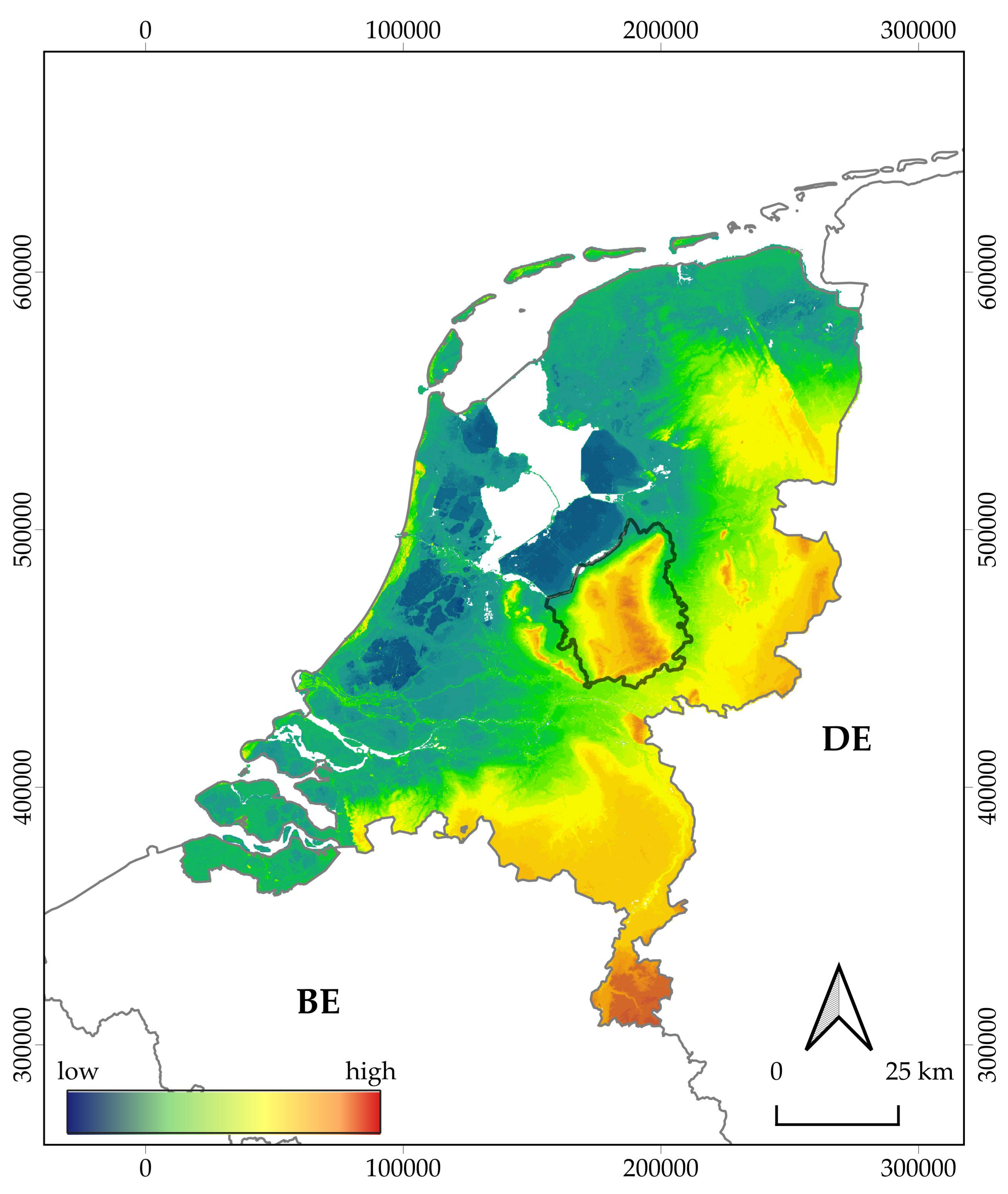
2. Research Area and Archaeological Classes

The archaeological and LiDAR data used in this research derive from a region known locally as the Veluwe, in the western part of the province of Gelderland in the Netherlands (Figure 1). This region (ca. 2200 km²) consists of multiple north–south orientated ice-pushed ridges, separated by relatively flat valleys originating from the Saale glacial period (ca. 350,000 to 130,000 BCE). In later periods, the area was partially covered with cover sand and drift-sand (i.e., aeolian sand) deposits [21,22]. Nowadays, the Veluwe is predominantly covered with forest and heath, interspersed with agricultural fields, variously sized areas of habitation and major and minor roads. The area holds one of the largest clusters of known archaeological objects in the Netherlands. The majority of the extant objects can be found in heathland or under forest cover [11]. While their location has certainly contributed to their present-day preservation, it also limits the detailed investigation of known sites and the survey of their surrounding landscape for potential new archaeological objects [23].

Two classes of archaeological objects are of interest for this research: prehistoric barrows and Celtic fields (Figure 2). These classes were chosen because these objects have been studied extensively in several recent archaeological projects [12,25,26], which generated up-to-date inventories of these object classes in the research area, their dating, and their state of preservation. Furthermore, barrows and Celtic fields are clearly visible in LiDAR data—contrary to in other remote sensing datasets or the situation in the field where these objects are generally hard to discern due to the fact that the majority of the extant objects are located under forest cover [23,27]. This makes these classes good candidates for object detection tasks. The majority of barrows on the Veluwe—small, round, or oval-shaped earthen mounds that demarcate the burial place of a select group of people—were erected and used in the Neolithic and Bronze Age (between 2800 and 1400 cal BCE; refs. [26,28]). Celtic fields are a later prehistoric (late Bronze Age until the Roman Period; ca. 1100 cal BCE–200 CE) parcelling system composed of adjoining, roughly rectangular, embanked plots, which form a characteristic checker-board pattern in LiDAR data [25]. Barrows are examples of ‘discrete’ archaeological objects due to their convex, compact and localised shapes, while Celtic fields are examples of ‘landscape patterns’ [29,30] since they have a large-scale non-localised shape.

3. Related Work: The GIS-Based Measure

In the research on the Veluwe, barrows (i.e., discrete objects) are generally validated through hand corings (see [6,11]): the location (i.e., the central coordinate) of these objects is more informative than their extent (as shown by the predicted bounding boxes), especially as the appearance of objects in LiDAR data often differs from the real-world situation [32]. Celtic fields (i.e., landscape patterns) are instead generally validated through the additional analysis of remote sensing data, as validation in the field is often problematic due to the lack of clear traces and material culture [11]. Therefore, gaining additional information via the automated detection, e.g., on the extent and coverage of these objects, is more relevant, especially as this offers information that can be used to answer additional questions on, for instance, yield and demographics [25].

In both discrete objects and landscape patterns cases, these two types of validation have been developed to address specific archaeological goals by developing the GIS-based measure [6]. First, the GIS-based measure converts the predicted bounding boxes into geospatial vectors. Specifically, in the case of discrete objects, the detections are converted into points by taking the central coordinate (or centroid) of the bounding box. These points are then overlaid to a spatial layer of the test area previously divided into cells with sizes based on the average size of the archaeological objects in question. In this perspective, a detection has to be close enough to a ground truth, i.e., within the ground truth annotation, to be considered as a True Positive (TP), while the coverage of the produced bounding box is of less importance (see Figure 3). Subsequently, the number of TPs and False Positives (FPs) is determined by selecting all ’positive’ and ’negative’ grid cells that contain a detection by means of a GIS software (such as QGIS). Multiple detections in the same grid cell are individually counted. Finally, False Negatives (FNs) are computed (total number of barrows in the dataset minus TP) and True Negatives (TNs) (total negative grid cells minus FPs).

Conversely, when the detected objects concern landscape patterns (e.g., plots within a Celtic field), a different approach is taken. The bounding boxes are converted into polygons, and then overlaid to a spatial layer containing polygon features for all the Celtic fields in the test area, while the rest of the area is filled with a single ‘negative’ polygon (see Figure 4). The difference in square meters between these two layers is determined by ‘cutting’ the detected polygons from the spatial layer of the test area by means of a GIS software. This gives the amount of FN (remaining area of Celtic field) and the amount of TN (remaining area of ‘negative’ polygon) in square meters. In this case, both the location and coverage of the produced bounding boxes are regarded as important. TP is computed as the total area of Celtic fields in the test dataset minus FN, while FP as the total ’negative’ area in the test dataset minus TN.

4. Automatic Evaluation Measures

This section described the two automatic performance evaluation measures, called ‘centroid-based’ and ‘pixel-based’, and highlights the advantages of their use with respect to the IoU. The centroid-based measure is suited for discrete objects, while the pixel-based measure is tailored to landscape patterns. The pseudocodes of the algorithms to compute the centroid-based and the pixel-wise show that these two measures are designed to be a fully automatic replacements of the GIS-based measure encoding the salient aspects of the archaeologists’ thinking process. All these measures take as input the bounding boxes predicted by an object detection method and output the number of TPs, FPs, TNs and FNs. These values are then used to compute metrics generally adopted to evaluate the performance of object detection methods, such as Precision and Recall.

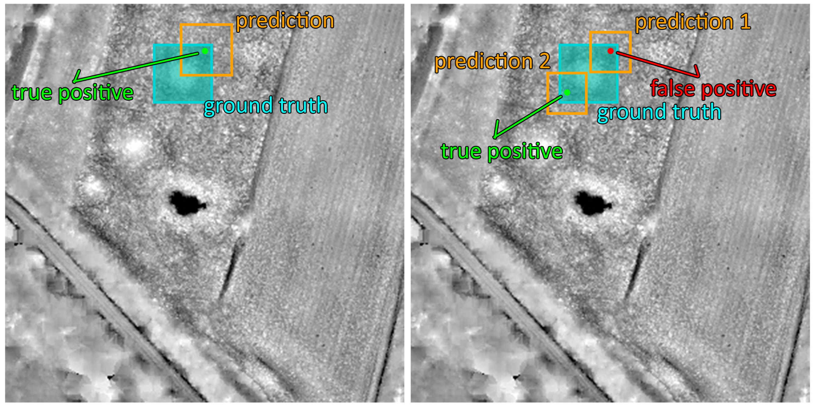
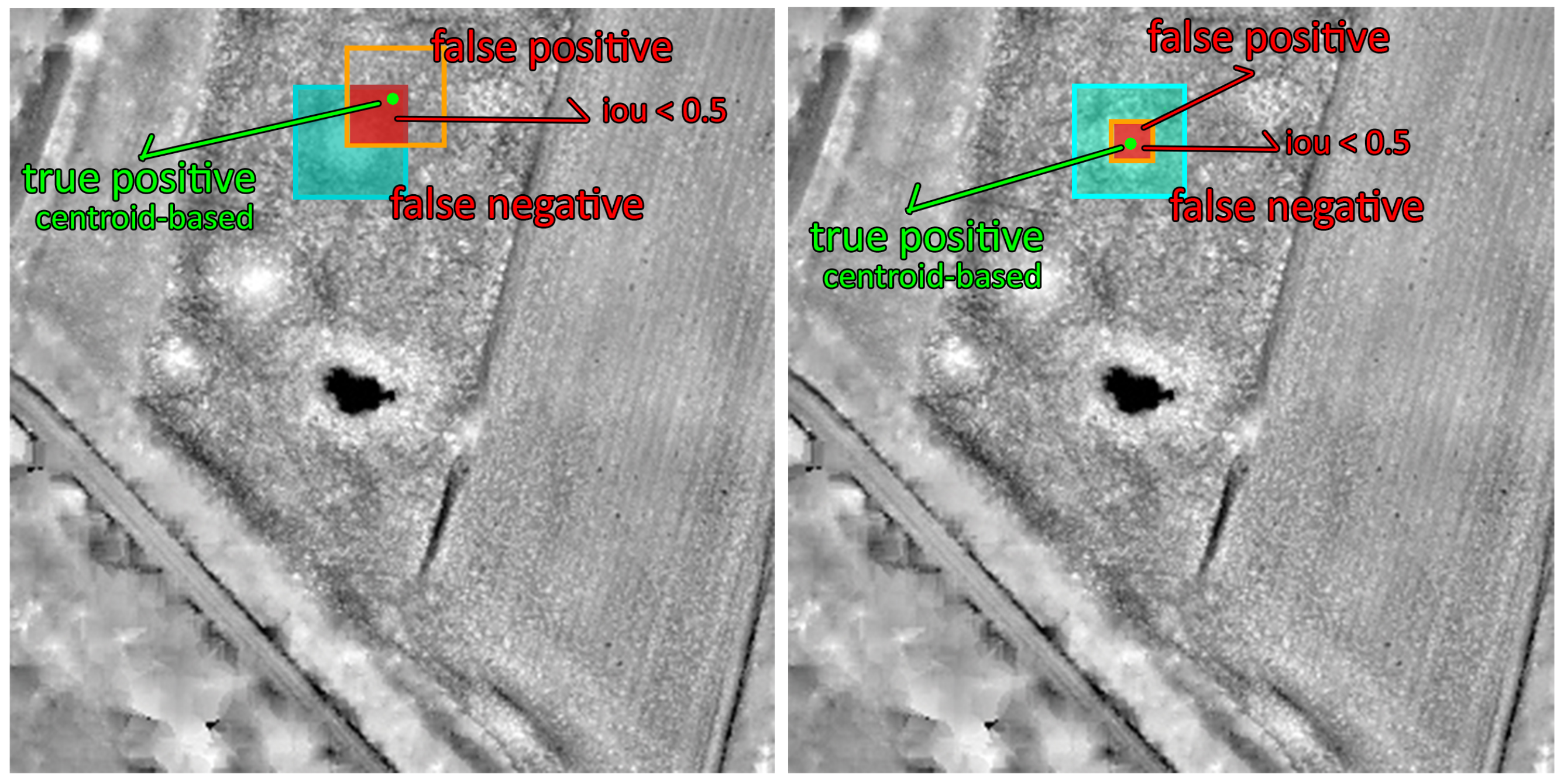
4.1. Centroid-Based Measure

The centroid-based measure, tailored to discrete objects, provides a quantitative evaluation of the spatial relationship between predicted and ground truth objects in order to reflect the archaeologists’ expectation of detecting an object close enough to where it should be, i.e., within the corresponding ground truth annotation. This spatial relationship is quantified by considering if the centroid of each predicted object’s bounding box is inside the closest ground truth bounding box. Specifically, as shown in Algorithm 1, a prediction is considered as a TP if the predicted object’s centroid falls inside the area of (at least) one ground truth’s bounding box; otherwise, the prediction is considered as an FP. The association between a ground truth object and its eventual prediction is exclusive: whenever a TP prediction is associated with a ground truth, the latter cannot be associated with any further predictions. This guarantees that, if there are two or more distinct predictions, the centroids of which fall inside the same ground truth’s bounding box, only one is considered as a TP, while the others are computed as FPs. Since this circumstance only occurs sporadically in our experiments, we decided to neglect additional efforts to select the ‘best match’, i.e., the detection closest to the centroid, as this would impact computational costs and memory usage, while providing negligible advantage to performances. Consequently, we adopted a ‘first-come, first-selected’ approach. Conversely, all the other ground truth bounding boxes, which do not have an ‘associated’ prediction,—i.e., a predicted object whose centroid falls inside the ground truth’s bounding box—are considered as an FN (see Figure 5).

Algorithm 1: Centroid-based measure

The centroid-based measure gives more importance to the location (i.e., the central coordinate) of objects than their extent (as shown by the predicted bounding boxes) as described in [6]. This crucial aspect is not grasped by the IoU that computes the extension of the overlap between the predicted and the ground truth bounding boxes. Figure 6 shows two examples that highlight the advantages of the employment of the centroid-based measure with respect to the IoU.

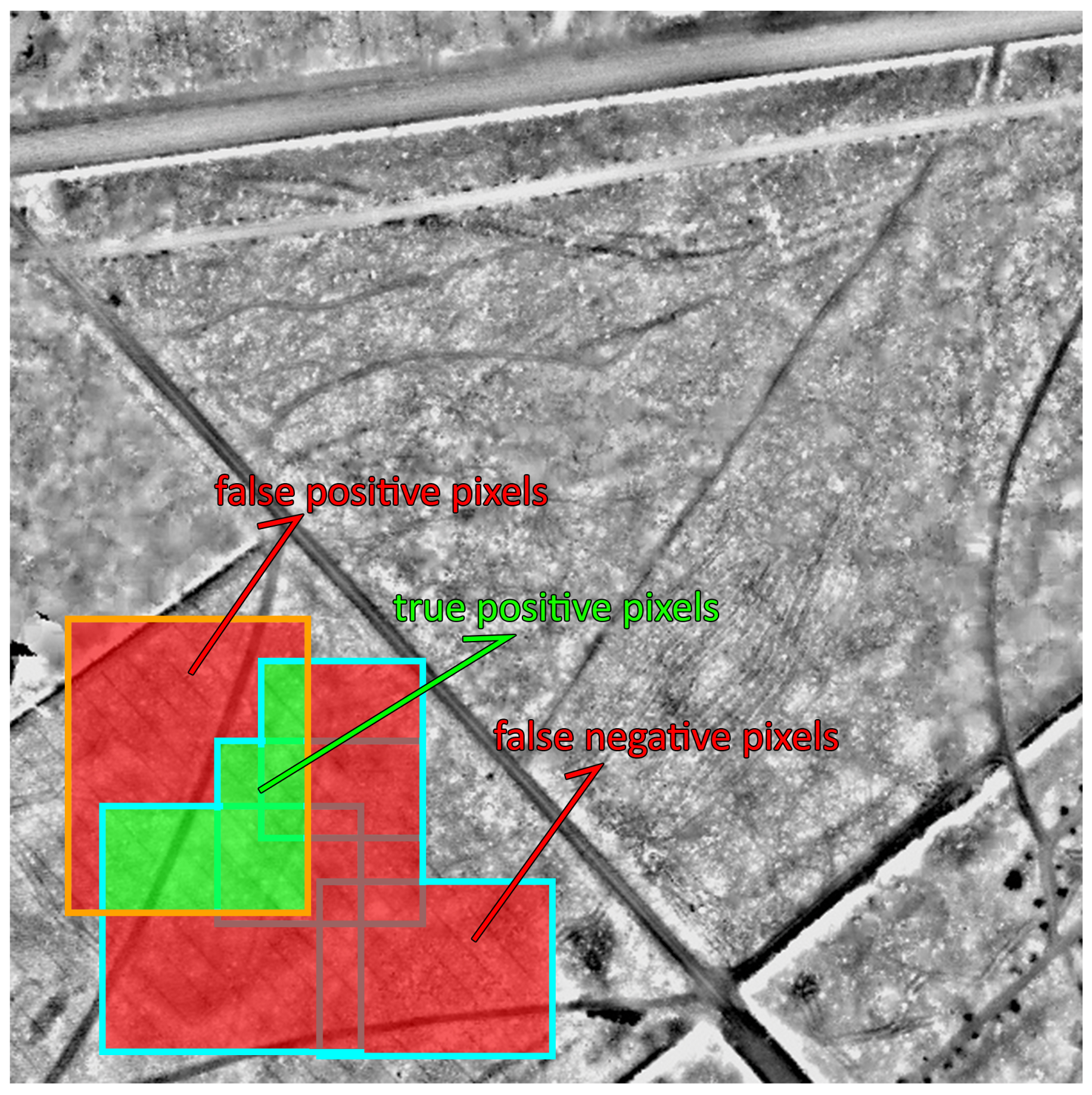
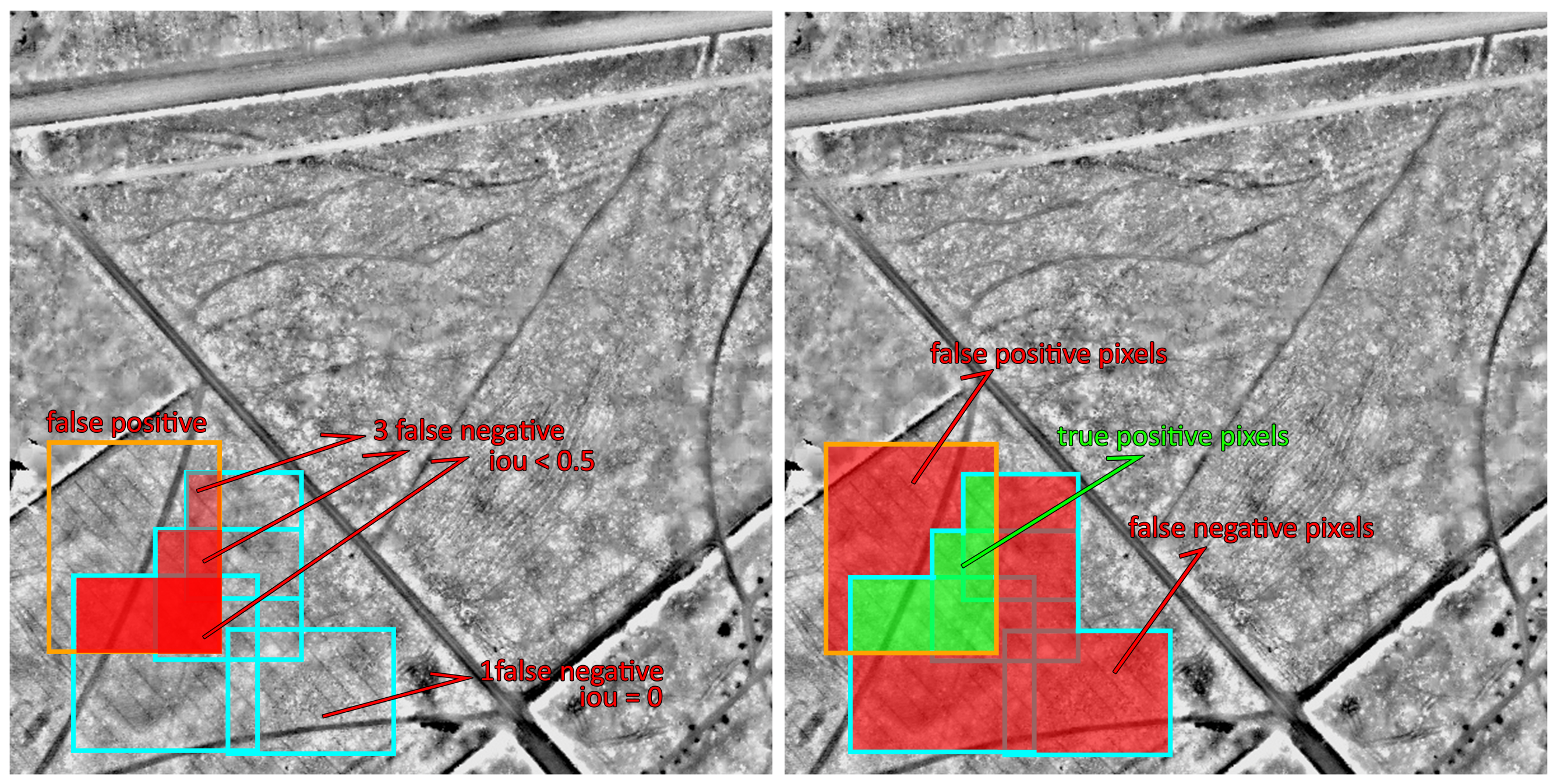
4.2. Pixel-Based Measure

The pixel-based measure, suited for landscape patterns [29,30] such as Celtic fields, considers the object detection task as the classification of each pixel of an image. Specifically, as shown in Algorithm 2, for each class, a binary mask is calculated of both the ground truth annotations and predicted objects. The mask has the same width and height of the original image and represents the presence (or absence) of all the objects of the given class, as it assumes for each corresponding position the binary value 1 if in that position an object instance is present, or conversely the binary 0 whenever it is not. Then, the ground truth mask and the prediction mask are compared on a pixel-wise level, using an $AND$ (bit-wise) operator: each pixel where both masks contain the binary value 1 (presence of an archaeological object) is considered as a TP, while pixels with binary value 1 in the ground truth mask and binary value 0 in the prediction mask are considered as an FN, and conversely pixels with binary value 0 in the ground truth mask and binary value 1 in the prediction mask are considered as FPs.

Algorithm 2: Pixel-based measure

Since the pixel-based measure works by definition in a pixel-wise fashion, a single bounding box can partly be counted as a TP and as an FP, depending on the overlap with the ground truth (see Figure 7). The IoU is not the ideal measure for such patterns because it does not take into account the amount of coverage between the predicted and the ground truth bounding boxes at a pixel level, but it considers if the whole predicted bounding box is a TP or an FP: if the ratio between the corresponding coverage (intersection) and their union is greater than a given threshold, it is a TP; otherwise, it is an FP (see Figure 8 and Section 7).

5. Experimental Setup

In this section, the experimental setup, designed for assessing the discrepancies among the two automatic measures (see Section 4) and the semi-automatic (GIS-based) measure (see Section 3), is described. The section is organised as follows: Section 5.1 provides a detailed description of the datasets used to train, validate and test the object detection networks. In Section 5.2, the experimental methodology, in which nine object detection networks are trained and tested on the same LiDAR dataset, is presented.

5.1. Datasets

Starting in 1997, the Dutch Directorate-General for Public Works and Water Management has commissioned nation-wide LiDAR coverage for the Netherlands. In this research, the second generation of this LiDAR dataset, called the Actueel Hoogtebestand Nederland 2 (AHN2), is used (See

Table 1. The parameters of the LiDAR data used in this research, after Ref. [35].

Parameters AHN2 LiDAR Data
purpose	water management
time of data acquisition	April 2010
equipment	RIEGL LMS-Q680i Full-Waveform
scan angle (whole FOV)	45°
flying height above ground	600 m
speed of aircraft (TAS)	36 m/s
laser pulse rate	100,000 Hz
scan rate	66 Hz
strip adjustment	yes
filtering	yes
interpolation method	moving planes
point-density (pt per sq m)	6–10
DTM-resolution	0.5 m

for an overview of the parameters of the LiDAR data). This dataset is freely available as an interpolated Digital Terrain Model (DTM), disseminated in GeoTIFF raster images (or tiles) measuring 10,000 by 12,500 pixels (5 km by 6.25 km), from the online repository PDOK [24].

To assemble the datasets, 16 GeoTIFF tiles were downloaded and processed with a Fill_nodata tool in QGIS 3.4 Madeira [33] to reduce the number of no-data points. Subsequently, the tiles were visualised with the Simple Local Relief Model visualisation [31] from the Relief Visualisation Toolbox 1.3 [34]. Thirteen tiles were selected as training data, one tile as validation data and two tiles as test data. All tiles were sliced into subtiles of 600 by 600 pixels with 30 pixel overlap on all sides [6].

5.1.1. Training and Validation Datasets

The 14 tiles selected for training and validation were dissected into 5796 subtiles, of which only a minority contain an archaeological object of interest. The subtiles that did contain barrows and/or Celtic fields were selected and labelled with LabelImg [36], a graphical image annotation tool to generate object bounding boxes (Figure 2). Every individual barrow was annotated, resulting in 1340 examples. In the case of Celtic fields, every individual plot was labelled, resulting in 1382 examples. The objects included in the datasets represent both clear and less conspicuous examples, in various states of preservation (e.g., a portion of the extant barrows has been physically reconstructed decades ago in an attempt to preserve them). In the case of overlapping objects, e.g., a barrow within a Celtic field, the concerned subtile was excluded from the training dataset, as this might generate complications with the pixel-based evaluation measure (see Section 4.2). The developed training dataset contains 993 subtiles, while the validation dataset—used to monitor the network during training—includes 88 subtiles (

Table 2. The datasets used in this research.

Dataset	Subtiles	Barrows	Celtic Fields	Objects
training	993	1213	1318	2531
validation	88	127	64	191
test	825	130	997	1127

).

5.1.2. Test Dataset

For the test dataset, two separate areas on the Veluwe were selected: both have been extensively researched in the (recent) past [25,26] and contain multiple examples of the archaeological classes of interest, in various states of preservation. Furthermore, these two areas contain a representative sample of the different types of land-use and terrain present on the Veluwe.

To create the dataset, all subtiles (828 in total) of the two areas were collected and manually annotated by two expert researchers: both with ample experience in analysing LiDAR data and considerable knowledge of the archaeology of the research area. These annotations were also compared and supplemented with information on extant archaeological objects on record in any of the Dutch national archaeological databases [37]. Again, subtiles containing overlapping archaeological objects were excluded (see above).

The resulting test dataset (see Table 2) consists of 825 subtiles of which 164 (19.8%) contain a total of 1127 examples, split into 130 barrows and 997 Celtic field plots (the total area covered by Celtic fields equals circa 2.42 km² spread over 66 demarcated areas). The other 661 subtiles (80.2%) do not contain any archaeological object from the two classes of interest. The resulting ratio of positive and negative subtiles (i.e., with or without archaeological objects of interest respectively) of about 1:5 (positive:negative) in the test dataset accurately represents the real-world situation of scarce archaeological objects in different types of complex and dynamic terrain [6].

5.2. Experimental Methodology

Object detection is a popular and fast evolving field within Deep Learning research. Consequently, original, potentially ground-breaking research is published regularly and comparing all developed networks and architectures is out of the scope of this research. Furthermore, developing a network from scratch is regarded as unnecessary and inefficient. Therefore, Detectron2 [38], a Pytorch-based library developed by Facebook AI Research (FAIR), is used in this research. This library aims towards an enhanced flexibility and extensibility through a proper re-factored modular design and the ability to provide fast training on single or multiple GPU servers. Moreover, it fills the gap between research (development) and industry (use) by providing different implementations of state-of-the-art object detection networks and algorithms. Detectron2 was initially used to rapidly construct and explore different architectures and combinations of pre-trained models. Preliminary experiments with different approaches (e.g., RetinaNet-based single-shot detection models) did not result in any significant gain, and eventually the choice was made to settle on a single, state-of-the-art object detection network, Faster R-CNN [39], to test the proposed measures.

5.2.1. Faster R-CNN

Faster R-CNN is an object detection network, and one of the latest evolutions of the R-CNN architecture [40]. This ’two-stage’ detector consists of two parts: a region proposal network (RPN; a small fully connected network) that generates the object proposals, while feature extraction and classification are done by the Fast R-CNN detector [41]. An input image is passed through a backbone, pre-trained CNN that uses an intermediate layer as a convolutional feature extractor. The extracted feature map is sent as input to the RPN, which in turn outputs a set of rectangular object proposals, each with a likelihood that the proposal contains a relevant object. This is done by generating so-called anchor boxes (pre-fixed temporary bounding boxes) with three different scales and three aspect ratios (1:1, 1:2 and 2:1) at set intervals (called stride). The main task of the RPN is to deliver an ‘attention mechanism’ by providing a set of relevant object proposals. These ‘proposals’ are then filtered based on their ‘objectness score’, i.e., the probability that a proposal represents an object, and passed as input to the Region of Interest (RoI) pooling module. Instead of trying to classify each proposal, the RoI pooling module improves the training efficiency by extracting a fixed-length feature vector for each region proposal with the aim of reusing these convolutional feature maps as input of a region-based object detection network (Fast R-CNN). The network classifies the fixed-length features into a given number of classes by returning class scores and a background class, and uses a linear regressor to tighten the bounding box to fit the true sizes of the object [39]. Based on a set confidence score threshold, object proposals are discarded or given as output of the network. Both the RPN and Fast R-CNN are trained simultaneously during the training of Faster R-CNN [42].

5.2.2. Faster R-CNN Implementations

In our experiments, nine different Faster R-CNN networks were used (see also Figure 9 and Figure 10). In these models, the backbone CNN, the feature extraction and the training regime were varied. These variations will be explained in the following.

The main difference among Faster R-CNN networks is the backbone, pre-trained CNN (i.e., the first part of Faster R-CNN), the principal role of which is to extract the feature map for the following components. In this research, different versions of the ResNet-based architecture [43] were used. These CNNs are composed of alternations of stem blocks and bottleneck blocks. While the former is basically a down-sampling convolutional block, the latter introduces shortcut convolutions to combine input and output features. By using a combination of different block sizes (i.e., numbers of layers inside a block) and numbers of blocks, different ResNet-based architectures have been developed [43]. ResNet50 (R_50), ResNet101 (R_101) and ResNeXt-101-32x8d (X_101_32x8d) were used. The latter architecture basically performs a multi-path parallel convolution through several ResNet blocks and then merges the results [44].

Moreover, the backbone CNNs in our different Faster R-CNN networks were further varied with three different modifications (C4, FPN and DC5) to the feature extraction process:

• C4: uses the original approach of the Faster R-CNN paper, with ResNet conv4 backbone and conv5 head [39];
• FPN (Feature Pyramid Network): adds a layer that can extract multi-scale feature maps, thereby taking advantage of different receptive fields [45];
• DC5 (Dilated-C5): introduces dilations in Resnet conv5 backbone, i.e., a dedicated convolutional layer with the ability to change its sampling grid in order to enlarge its receptive field [46].

Finally, the different backbone CNNs have been pre-trained with different training regimes, either 1x or 3x. In the former, the CNN has been pre-trained for 12 epochs on the Microsoft COCO dataset [17], while the latter concerned 37 epochs. In Section 6.1, the results of the different networks are presented.

5.2.3. Hardware Setup

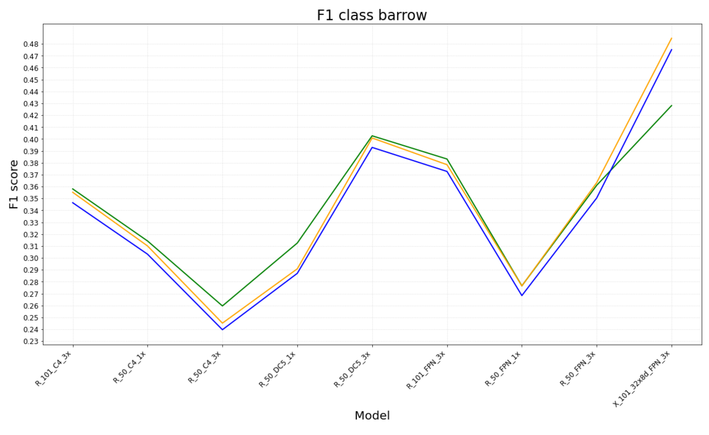
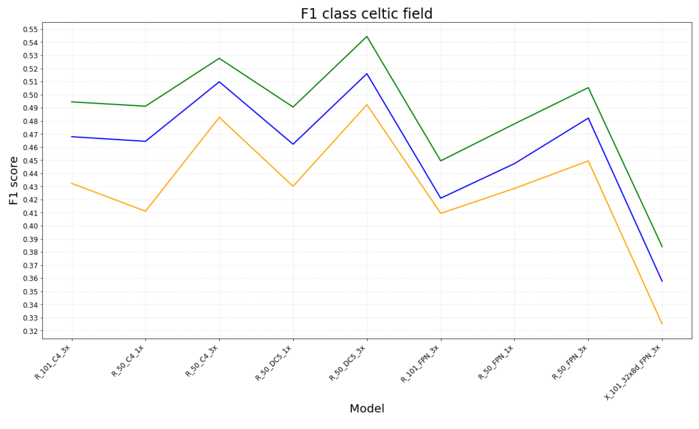
The experiments with the different Faster R-CNN networks were run on a 64 GB RAM Dual Intel Xeon 4114 machine, equipped with four NVIDIA GeForce RTX 2080Ti GPUs. Typical training time for each model took between 10 and 40 minutes, depending on the exact number of epochs. Although Detectron2 offers many options to customise various hyperparameters to refine a model’s behaviour—either in the training or testing phase—in this research, most of the default configurations and parameters were retained. Therefore, the DefaultTrainer class provided in Detectron2 [38] was used. In addition, the maximum number of iterations was set to 10,000, and the base learning rate to $0.01$. To periodically evaluate the model on the validation dataset, the evaluation period was set to 1000. As the implementation did not make use of ’early stopping’, a method was developed and implemented to save the model, through a ’hook’ subclass, at several points during training, to choose a point in the training process with the best validation/training loss curve trade-off. Finally, to increase the models’ precision, the confidence threshold was adjusted to $0.8$ [39]. While different data augmentation techniques were experimented with, empirically, it was determined that the default augmentations (i.e., resize and flip) were the most effective.

6. Results

The following paragraph describes the experimental results by comparing the performance—gained from using the different evaluation measures—of the nine object detection networks. The discrepancies among the two automatic evaluation measures (centroid-based and pixel-based) and the semi-automatic GIS-based measure [6] are then explored. In Section 7, general trends within the results will be discussed and the effectiveness of the two automatic evaluation measures to resemble the archaeologists’ thinking process—as distilled in the GIS-based measure—and the applicability for archaeological research are considered.

6.1. Experimental Results

Experiments were performed to assess the ability of the two proposed automatic measures to approximate the semi-automatic (GIS-based) measure developed by archaeologists [6]. To this aim, nine different networks, based on the Faster R-CNN architecture, were trained and tested on the same LiDAR dataset containing archaeological objects. Specifically, the following steps were performed and the obtained experimental results were used to construct different figures.

i

Each trained model was evaluated on the test dataset;

ii

The predictions of each model were given as input to the two automated measures (see Section 4) and to the semi-automatic (GIS-based) measure (see Section 3);

iii

The number of TP, FP and TN for each class (barrow and Celtic field) were obtained from each evaluation measure;

iv

Based on these values, F1-scores (for each class and a mean) were computed per model, for each evaluation measure.

Figure 9 and Figure 10 show that the centroid-based and the pixel-based have the same trend of the GIS-based measure, demonstrating that the two novel automatic measures encode the salient aspect of the archaeological thinking process distilled into the semi-automatic GIS-based measure. Specifically, the average discrepancy between the centroid-based and the GIS-based for barrows (Figure 9) is less than $1\%$ and the average discrepancy between the pixel-based and GIS based for Celtic fields (Figure 10) is less than $3\%$.

7. Discussion

The results (Figure 9 and Figure 10) show a high similarity in the performance (F1-score) calculated with the different evaluation measures, although some variation can be detected among the nine Faster R-CNN networks and can be explained by a difference in the capacities of individual models to correctly distinguish and delimit objects, especially small objects (see Figure 11). An in-depth analysis of the results, based on the visual inspection of overlays (see, for instance, Figure 11) containing the prediction results and the ground truth, has shown several causes for the observed variation among the different evaluation measures. To start with, the graph for discrete objects (Figure 9) shows that the pixel-based measure deviates the most from the general trend, which is apparent among the other evaluation measures. This is most probably caused by the fact that the pixel-based measure is sensitive to wrongly approximated bounding boxes (see Figure 11): if the predicted bounding box is slightly different in size or shape, as compared to the ground truth, FP and FN are created, even though the presence and location of a particular object is correctly predicted. Then, on the other hand, bounding boxes are of no relevance for the centroid-based approach wrongly approximated as only the position of the centroid in relation to the ground truth annotation is determining. The same goes for the GIS-based measure, where only the location of the bounding box, and not the extent, is of relevance. Several specific discrepancies, for instance for the pixel-based measure for model X_101_32x8d_FPN_3x on barrows (Figure 9), is presumably caused by this problem, in combination with a high loss (error) in the bounding box regressor (see [39]), which is responsible for correctly approximating bounding boxes.

Furthermore, a larger variation can be observed among performance in the Celtic field class (Figure 10). The lines depicting the different measures clearly deviate, while, in the other plot, the lines are much closer together (Figure 9), although the general trend is the same. A possible cause of the difference in performance between the centroid-based measure, which is consistently lower, and the other measures lie in the fact that many of the ground truth bounding boxes overlap (see Figure 12). As explained in Section 4.1, the association between a ground truth and a prediction is exclusive in this measure. Therefore, in the case of many overlapping ground truth bounding boxes, the centroid-based measure will produce more FPs, resulting in a lower performance. Furthermore, in the case of the pixel-based and GIS-based measure, a single bounding box can partly be counted as TP and as FP, depending on the overlap with the ground truth. Conversely, the pixel-based measure gives consistent higher performance than the GIS-based measure. This might be caused by a difference in scale: the pixel-based measure calculates performance based on pixels of 0.5 meters in size, while the GIS-based measure uses the amount of square meters.

Archaeological Implications

Machine Learning is progressively being used to automatically detect archaeological objects in remote sensing data. Research has shown, however, that this particular task is not as straightforward as more general object detection tasks, such as finding people or household objects in photographs [12]. Consequently, standard evaluation measures are ill-fitted for this task due to inherent differences between archaeological objects and more common objects and their disregard of geospatial information. Therefore, the evaluation measures presented in this paper, which are geared towards archaeology, give a better indication of the performance of archaeological object detection methods and make their application better suited for archaeological research, encouraging their wide-spread application within wider archaeological research frameworks and heritage management [47]. More generally, these automated detection methods can alleviate the labor and time-investment of the analysis of remote sensing data and offer opportunities to efficiently investigate archaeological hypotheses on a landscape scale. Finally, the ability to rapidly detect objects in remote sensing data might also prevent the irretrievable loss of archaeological sites and information due to the ever-increasing threat to archaeology, for instance due to agriculture and urban development [48], but also looting and systematic and deliberate destruction [49].

8. Conclusions

The experimental results showed that the two proposed automatic measures encode what is salient and important for archaeological research. This is a crucial requirement for any measure to become widely accepted in the archaeological community as a standard evaluation tool for comparing different archaeological object detection workflows. The centroid-based and the pixel-based measures provide the necessary archaeological information for further (field) research. We envision that the community will consider these two measures as a standard performance evaluation tool from now on. This research also shows the necessity of interaction between archaeological and machine learning researchers in order to obtain satisfactory results across both the disciplines (see also [27,50]). A fundamental aspect in designing and implementing the next generation of archaeological object detection methods will be the increase in the role of the archaeologist in the learning process to provide domain knowledge to the machine [12]. A possible method to enable the archaeologist to provide continuous feedback to the machine depending on the correctness of its predictions are active learning-based approaches [51]. These will also enable us to overcome the need for a large amount of labelled training data, which is one of the main challenges in archaeological automated detection [52]. Active learning takes advantage of the availability of unlabelled data by posing queries to archaeologists about the data needed to be labelled by them and is one of the instances of the human-in-the-loop paradigm, which contributes to make machine learning models more interpretable [53,54]. Based on these considerations, we argue that the adoption of a standard evaluation measure to assess the performance of archaeological object detection methods will enable a cross-study comparison and a cross-fertilisation between scholars in machine learning and archaeology, which in turn will encourage the development of novel human-centred machine learning methods for the detection of archaeological objects.

References

1. Orengo, H.A.; Conesa, F.C.; Garcia-Molsosa, A.; Lobo, A.; Green, A.S.; Madella, M.; Petrie, C.A. Automated detection of archaeological mounds using machine-learning classification of multisensor and multitemporal satellite data. Proc. Natl. Acad. Sci. USA 2020, 117, 18240–18250. [Google Scholar] [CrossRef] [PubMed]
2. Bundzel, M.; Jaščur, M.; Kováč, M.; Lieskovský, T.; Sinčák, P.; Tkáčik, T. Semantic Segmentation of Airborne LiDAR Data in Maya Archaeology. Remote Sens. 2020, 12, 3865. [Google Scholar] [CrossRef]
3. Somrak, M.; Džeroski, S.; Kokalj, Z. Learning to Classify Structures in ALS-Derived Visualizations of Ancient Maya Settlements with CNN. Remote Sens. 2020, 12, 2215. [Google Scholar] [CrossRef]
4. Soroush, M.; Mehrtash, A.; Khazraee, E.; Ur, J.A. Deep Learning in Archaeological Remote Sensing: Automated Qanat Detection in the Kurdistan Region of Iraq. Remote Sens. 2020, 12, 500. [Google Scholar] [CrossRef] [Green Version]
5. Trier, Ø.D.; Salberg, A.B.; Pilø, L.H. Semi automatic mapping of charcoal kilns from airborne laser scanning data using deep learning. In CAA 2016: Oceans of Data. Proceedings of the 44th Conference on Computer Applications and Quantitative Methods in Archaeology; Matsumoto, M., Uleberg, E., Eds.; Archaeopress: Oxford, UK, 2018; pp. 219–231. [Google Scholar]
6. Verschoof-van der Vaart, W.B.; Lambers, K.; Kowalczyk, W.; Bourgeois, Q.P. Combining Deep Learning and Location-Based Ranking for Large-Scale Archaeological Prospection of LiDAR Data from The Netherlands. ISPRS Int. J. Geo Inf. 2020, 9, 293. [Google Scholar] [CrossRef]
7. Zingman, I.; Saupe, D.; Penatti, O.A.B.; Lambers, K. Detection of fragmented rectangular enclosures in very-high-resolution remote sensing images. IEEE Trans. Geosci. Remote Sens. 2016, 54, 4580–4593. [Google Scholar] [CrossRef]
8. Simonyan, K.; Zisserman, A. Very Deep Convolutional Networks for Large-Scale Image Recognition. In Proceedings of the 3rd International Conference on Learning Representations, ICLR 2015, San Diego, CA, USA, 7–9 May 2015. [Google Scholar]
9. Ronneberger, O.; Fischer, P.; Brox, T. U-Net: Convolutional Networks for Biomedical Image Segmentation. In Medical Image Computing and Computer-Assisted Intervention—MICCAI 2015; Navab, N., Hornegger, J., Wells, W., Frangi, A., Eds.; Springer: Cham, Switzerland, 2015. [Google Scholar] [CrossRef] [Green Version]
10. He, K.; Gkioxari, G.; Dollar, P.; Girshick, R. Mask R-CNN. In Proceedings of the IEEE International Conference on Computer Vision (ICCV), Venice, Italy, 22–29 October 2017. [Google Scholar]
11. Lambers, K.; Verschoof-van der Vaart, W.B.; Bourgeois, Q.P.J. Integrating Remote Sensing, Machine Learning, and Citizen Science in Dutch Archaeological Prospection. Remote Sens. 2019, 11, 794. [Google Scholar] [CrossRef] [Green Version]
12. Verschoof-van der Vaart, W.B. Learning to Look at LiDAR. Combining CNN-Based Object Detection And GIS for Archaeological Prospection in Remotely-Sensed Data. Ph.D. Thesis, Leiden University, Leiden, The Netherlands, 2022. Available online: https://hdl.handle.net/1887/3256824 (accessed on 27 March 2022).
13. Fiorucci, M.; Khoroshiltseva, M.; Pontil, M.; Traviglia, A.; Del Bue, A.; James, S. Machine Learning for Cultural Heritage: A Survey. Pattern Recognit. Lett. 2020, 133, 102–108. [Google Scholar] [CrossRef]
14. Randrianarivo, H.; Le Saux, B.; Ferecatu, M. Urban structure detection with deformable part-based models. In Proceedings of the 2013 IEEE International Geoscience and Remote Sensing Symposium—IGARSS, Melbourne, VIC, Australia, 21–26 July 2013; pp. 200–203. [Google Scholar]
15. Everingham, M.; Eslami, S.M.A.; Van Gool, L.; Williams, C.K.I.; Winn, J.; Zisserman, A. The Pascal Visual Object Classes Challenge: A Retrospective. Int. J. Comput. Vis. 2015, 111, 98–136. [Google Scholar] [CrossRef]
16. Ding, J.; Xue, N.; Xia, G.; Bai, X.; Yang, W.; Yang, M.Y.; Belongie, S.J.; Luo, J.; Datcu, M.; Pelillo, M.; et al. Object Detection in Aerial Images: A Large-Scale Benchmark and Challenges. IEEE Trans. Pattern Anal. Mach. Intell. 2021, 1. [Google Scholar] [CrossRef]
17. Lin, T.Y.; Maire, M.; Belongie, S.; Hays, J.; Perona, P.; Ramanan, D.; Dollár, P.; Zitnick, C.L. Microsoft COCO: Common Objects in Context. In Computer Vision—ECCV 2014; Fleet, D., Pajdla, T., Schiele, B., Tuytelaars, T., Eds.; Springer International Publishing: Cham, Switzerland, 2014; pp. 740–755. [Google Scholar]
18. Rezatofighi, S.H.; Tsoi, N.; Gwak, J.; Sadeghian, A.; Reid, I.D.; Savarese, S. Generalized Intersection Over Union: A Metric and a Loss for Bounding Box Regression. In Proceedings of the 2019 IEEE/CVF Conference on Computer Vision and Pattern Recognition (CVPR), Long Beach, CA, USA, 15–20 June 2019; pp. 658–666. [Google Scholar]
19. Gillings, M.; Hacigüzeller, P.; Lock, G. Archaeology and spatial analysis. In Archaeological Spatial Analysis: A Methodological Guide; Gillings, M., Hacigüzeller, P., Lock, G., Eds.; Routledge: New York, NY, USA, 2020; Chapter 1; pp. 1–16. [Google Scholar]
20. Yoo, D.; Kweon, I.S. Learning Loss for Active Learning. In Proceedings of the 2019 IEEE/CVF Conference on Computer Vision and Pattern Recognition (CVPR), Long Beach, CA, USA, 15–20 June 2019. [Google Scholar]
21. Berendsen, H.J.A. De Vorming van het Land. Inleiding in de Geologie en de Geomorfologie, 4th ed.; Koninklijke Van Gorcum: Assen, The Netherlands, 2004. [Google Scholar]
22. Verschoof-van der Vaart, W.B.; Lambers, K. Learning to look at LiDAR: The use of R-CNN in the automated detection of archaeological objects in LiDAR data from the Netherlands. J. Comput. Appl. Archaeol. 2019, 2, 31–40. [Google Scholar] [CrossRef] [Green Version]
23. Kenzler, H.; Lambers, K. Challenges and Perspectives of Woodland Archaeology Across Europe. In CAA2014: 21st Century Archaeology, Concepts, Methods and Tools. Proceedings of the 42nd Annual Conference on Computer Applications and Quantitative Methods in Archaeology; Giligny, F., Djindjian, F., Costa, L., Moscati, P., Robert, S., Eds.; Archaeopress: Oxford, UK, 2015; pp. 73–80. [Google Scholar]
24. Nationaal Georegister. Publieke Dienstverlening Op de Kaart (PDOK). 2021. Available online: https://www.pdok.nl/ (accessed on 27 March 2022).
25. Arnoldussen, S. The Fields that Outlived the Celts: The Use-histories of Later Prehistoric Field Systems (Celtic Fields or Raatakkers) in the Netherlands. Proc. Prehist. Soc. 2018, 84, 303–327. [Google Scholar] [CrossRef] [Green Version]
26. Bourgeois, Q.P.J. Monuments on the Horizon. The Formation of the Barrow Landscape throughout the 3rd and 2nd Millennium BC; Sidestone Press: Leiden, The Netherlands, 2013. [Google Scholar]
27. Verschoof-van der Vaart, W.B.; Lambers, K. Applying automated object detection in archaeological practice: A case study from the southern Netherlands. Archaeol. Prospect. 2021, 29, 15–31. [Google Scholar] [CrossRef]
28. Bourgeois, Q.P.J.; Fontijn, D.R. The Tempo of Bronze Age Barrow Use: Modeling the Ebb and Flow in Monumental Funerary Landscapes. Radiocarbon 2015, 57, 47–64. [Google Scholar] [CrossRef] [Green Version]
29. Davis, D.S. Theoretical Repositioning of Automated Remote Sensing Archaeology: Shifting from Features to Ephemeral Landscapes. J. Comput. Appl. Archaeol. 2021, 4, 94–109. [Google Scholar] [CrossRef]
30. Traviglia, A.; Torsello, A. Landscape Pattern Detection in Archaeological Remote Sensing. Geosciences 2017, 7, 128. [Google Scholar] [CrossRef] [Green Version]
31. Hesse, R. LiDAR-derived Local Relief Models—A new tool for archaeological prospection. Archaeol. Prospect. 2010, 17, 67–72. [Google Scholar] [CrossRef]
32. Opitz, R.; Cowley, D. Interpreting Archaeological Topography. Airborne Laser Scanning, 3D Data and Ground Observation; Oxbow Books: Oxford, UK; Oakville, ON, Canada, 2013. [Google Scholar]
33. QGIS Development Team. QGIS Geographic Information System. 2017. Available online: http://qgis.org (accessed on 27 March 2022).
34. Kokalj, Ž.; Hesse, R. Airborne Laser Scanning Raster Data Visualization: A Guide to Good Practice; Založba ZRC: Ljubljana, Slovenia, 2017. [Google Scholar]
35. van der Zon, N. Kwaliteitsdocument AHN-2; Technical Report; Rijkswaterstaat: Amersfoort, The Netherlands, 2013. [Google Scholar]
36. Tzutalin. LabelImg. Git Code. 2015. Available online: https://github.com/tzutalin/labelImg (accessed on 27 March 2022).
37. Rijksdienst voor het Cultureel Erfgoed. ArchIS and AMK. 2021. Available online: https://www.cultureelerfgoed.nl/onderwerpen/bronnen-en-kaarten/overzicht (accessed on 27 March 2022).
38. Wu, Y.; Kirillov, A.; Massa, F.; Lo, W.Y.; Girshick, R. Detectron2. 2019. Available online: https://github.com/facebookresearch/detectron2 (accessed on 27 March 2022).
39. Ren, S.; He, K.; Girshick, R.; Sun, J. Faster R-CNN: Towards Real-Time Object Detection with Region Proposal Networks. IEEE Trans. Pattern Anal. Mach. Intell. 2017, 39, 1137–1149. [Google Scholar] [CrossRef] [Green Version]
40. Girshick, R.; Donahue, J.; Darrell, T.; Malik, J. Rich feature hierarchies for accurate object detection and semantic segmentation. In Proceedings of the 2014 IEEE Conference on Computer Vision and Pattern Recognition, Columbus, OH, USA, 23–28 June 2014; pp. 580–587. [Google Scholar] [CrossRef] [Green Version]
41. Girshick, R. Fast R-CNN. In Proceedings of the 2015 IEEE International Conference on Computer Vision, Santiago, Chile, 7–13 December 2015; pp. 1440–1448. [Google Scholar] [CrossRef]
42. Tang, T.; Zhou, S.; Deng, Z.; Zou, H.; Lei, L. Vehicle Detection in Aerial Images Based on Region Convolutional Neural Networks and Hard Negative Example Mining. Sensors 2017, 17, 336. [Google Scholar] [CrossRef] [Green Version]
43. He, K.; Zhang, X.; Ren, S.; Sun, J. Deep Residual Learning for Image Recognition. In Proceedings of the 2016 IEEE Conference on Computer Vision and Pattern Recognition, Las Vegas, NV, USA, 27–30 June 2016; pp. 770–778. [Google Scholar]
44. Xie, S.; Girshick, R.; Dollár, P.; Tu, Z.; He, K. Aggregated Residual Transformations for Deep Neural Networks. arXiv 2016, arXiv:1611.05431. [Google Scholar]
45. Lin, T.Y.; Dollár, P.; Girshick, R.; He, K.; Hariharan, B.; Belongie, S. Feature Pyramid Networks for Object Detection. In Proceedings of the 2017 IEEE Conference on Computer Vision and Pattern Recognition (CVPR), Honolulu, HI, USA, 21–26 July 2017. [Google Scholar] [CrossRef] [Green Version]
46. Dai, J.; Qi, H.; Xiong, Y.; Li, Y.; Zhang, G.; Hu, H.; Wei, Y. Deformable Convolutional Networks. In Proceedings of the 2017 IEEE International Conference on Computer Vision, Venice, Italy, 22–29 October 2017. [Google Scholar]
47. Kermit, M.; Reksten, J.H.; Trier, Ø.D. Towards a national infrastructure for semi-automatic mapping of cultural heritage in Norway. In Oceans of Data. Proceedings of the 44th Conference on Computer Applications and Quantitative Methods in Archaeology; Matsumoto, M., Uleberg, E., Eds.; Archaeopress: Oxford, UK, 2018; pp. 159–172. [Google Scholar]
48. Bonhage, A.; Raab, A.; Eltaher, M.; Raab, T.; Breuß, M.; Schneider, A. A modified Mask region-based convolutional neural network approach for the automated detection of archaeological sites on high-resolution light detection and ranging-derived digital elevation models in the North German Lowland. Archaeol. Prospect. 2021, 28, 177–186. [Google Scholar] [CrossRef]
49. El-Hajj, H. Interferometric SAR and Machine Learning: Using Open Source Data to Detect Archaeological Looting and Destruction. J. Comput. Appl. Archaeol. 2021, 4, 47–62. [Google Scholar] [CrossRef]
50. Olivier, M.; Verschoof-van der Vaart, W.B. Implementing Advanced Deep Learning Approaches for Archaeological Object Detection in Remotely-Sensed Data: The Results of Cross-Domain Collaboration. J. Comput. Appl. Archaeol. 2021, 4, 274–289. [Google Scholar]
51. Tuia, D.; Ratle, F.; Pacifici, F.; Kanevski, M.F.; Emery, W.J. Active Learning Methods for Remote Sensing Image Classification. IEEE Trans. Geosci. Remote Sens. 2009, 47, 2218–2232. [Google Scholar] [CrossRef]
52. Trier, Ø.D.; Cowley, D.; Waldeland, A.U. Using deep neural networks on airborne laser scanning data: Results from a case study of semi-automatic mapping of archaeological topography on Arran, Scotland. Archaeol. Prospect. 2019, 26, 165–175. [Google Scholar] [CrossRef]
53. Bickler, S.H. Machine Learning Arrives in Archaeology. Adv. Archaeol. Pract. 2021, 9, 186–191. [Google Scholar] [CrossRef]
54. Cowley, D.; Banaszek, Ł; Geddes, G.; Gannon, A.; Middleton, M.; Millican, K. Making LiGHT Work of Large Area Survey? Developing Approaches to Rapid Archaeological Mapping and the Creation of Systematic National-scaled Heritage Data. J. Comput. Appl. Archaeol. 2020, 3, 109–121. [Google Scholar] [CrossRef] [Green Version]
Figure 1. The research area on a height model of the Netherlands (source of the background image and elevation model: Ref. [24], coordinates in Amersfoort/RD New, EPSG: 28992; after Ref. [6]).
Remotesensing 14 01694 g001
Figure 2. Excerpts of LiDAR data, visualised with a Simple Local Relief Model [31], showing: barrows (left) and Celtic fields (right). The bottom row shows the corresponding annotations (source of the elevation model: Ref. [24]).
Remotesensing 14 01694 g002
Figure 3. The semi-automatic GIS-based measure [6] for the archaeological evaluation of discrete objects: (Left) the detections (black) on the spatial layer with positive grid cells in blue () and negative grid cells in red (); (Right) results of the processing with detected barrows (TP) in blue (), missed barrows (FN) in yellow (), wrong detections (FP) in red () and remaining empty grid cells (TN) in green ().
Remotesensing 14 01694 g003
Figure 4. The semi-automatic GIS-based measure [6] for the archaeological evaluation of landscape patterns: (Left) the detection polygons (black) on the spatial layer with Celtic fields polygons in blue () and the ’negative’ polygon in red (); (Right) results of the processing with detected areas of Celtic field (TP) in blue (), missed areas of Celtic field (FN) in yellow (), wrong detections (FP) in red () and remaining area of ’negative’ area (TN) in green ().
Remotesensing 14 01694 g004
Figure 5. The centroid-based measure provides a quantitative evaluation of the spatial relationship between predicted and ground truth objects. (Left) A prediction is considered as a TP () if the predicted () object’s centroid falls inside the area of (at least) one ground truth’s bounding box (). (Right) If there are two or more distinct predictions whose centroids fall inside the same ground truth’s bounding box, only one is considered as a TP (), while the others are considered as FPs ().
Remotesensing 14 01694 g005
Figure 6. The IoU is not the ideal measure for the evaluation of discrete archaeological object methods since it does not consider the geographical position of the predicted bounding box in relation to the shapes or areas counting archaeological objects. (Left) The centroid-based measure considers, in line with the archaeologists’ thinking process, the prediction as a TP () since the centroid of the predicted () bounding box falls inside the ground truth’s bounding box (). On the other hand, the IoU considers the prediction as an FP () because the intersection between the two bounding boxes is less than 0.5 times their union (see e.g., PASCAL VOC [15]). (Right) another example where the centroid-based is able to correctly consider a prediction as a TP, while the IoU considers it as an FP (see Section 7).
Remotesensing 14 01694 g006
Figure 7. The pixel-based measure provides a quantitative evaluation of the coverage of the ground truth bounding boxes with the predicted ones. The figure shows that a polygon representing an archaeological landscape pattern (a Celtic field) is annotated using a series of overlapped bounding boxes (ground truth ). Each pixel of a predicted () bounding box is considered as a TP () if it belongs to one of the ground truth bounding boxes; otherwise, it is considered as FP (). The pixels of each ground truth bounding boxes that are not covered by any predicted bounding box are considered as FN () (see Section 7).
Remotesensing 14 01694 g007
Figure 8. The IoU is not the ideal measure for landscape patterns since it does not take into account the amount of coverage between the predicted and the ground truth bounding boxes at a pixel level, but it considers if the whole predicted bounding box is a TP or an FP. (Left) All the intersections between the predicted () bounding boxes and each ground truth’s () bounding box are less than 0.5 times the corresponding union. The prediction is therefore considered as FP () and all the ground truth’s bounding boxes are considered as FNs (). (Right) On the other hand, the pixel-based measure, in line with the archaeologists’ thinking process, considers the detection of landscape patterns as the classification of each pixel of an image: each pixel is therefore evaluated as TP, FP or TN without considering any threshold (see Figure 7 and Section 7).
Remotesensing 14 01694 g008
Figure 9. An experimental evaluation of the discrepancy between the centroid-based, in orange (), the pixel-based measure in green (), and the semi-automatic GIS-based measure, in blue (), employed to assess the detection performance of nine different object detection networks in identifying barrows. The centroid-based measure has the same trend of the GIS-based one. The average discrepancy between the two curves (orange and blue) is less than 1 % .
Remotesensing 14 01694 g009
Figure 10. An experimental evaluation of the discrepancy between the pixel-based measure, in green (), the centroid-based, in orange (), and the semi-automatic GIS-based measure, in blue (), employed to assess the detection performance of nine different object detection networks in identifying Celtic fields. The pixel-based measure has the same trend of the GIS-based one. The average discrepancy between the two curves (green and blue) is less than 3 % .
Remotesensing 14 01694 g010
Figure 11. A comparison between a barrow ground truth (left) and the prediction (right) obtained with the X_101_32x8d_FPN_3x model, showing a wrongly approximated bounding box.
Remotesensing 14 01694 g011
Figure 12. Celtic field ground truth (left) vs. prediction (right) obtained with the R_50_C4_3x model, showing a clear difference between the often overlapping, ground truth bounding boxes and the predicted bounding boxes.
Remotesensing 14 01694 g012