Abstract
Historical land cover (LC) maps are an essential instrument for studying long-term spatio-temporal changes of the landscape. However, manual labelling on low-quality monochromatic historical orthophotos for semantic segmentation (pixel-level classification) is particularly challenging and time consuming. Therefore, this paper proposes a methodology for the automated extraction of very-high-resolution (VHR) multi-class LC maps from historical orthophotos under the absence of target-specific ground truth annotations. The methodology builds on recent evolutions in deep learning, leveraging domain adaptation and transfer learning. First, an unpaired image-to-image (I2I) translation between a source domain (recent RGB image of high quality, annotations available) and the target domain (historical monochromatic image of low quality, no annotations available) is learned using a conditional generative adversarial network (GAN). Second, a state-of-the-art fully convolutional network (FCN) for semantic segmentation is pre-trained on a large annotated RGB earth observation (EO) dataset that is converted to the target domain using the I2I function. Third, the FCN is fine-tuned using self-annotated data on a recent RGB orthophoto of the study area under consideration, after conversion using again the I2I function. The methodology is tested on a new custom dataset: the ‘Sagalassos historical land cover dataset’, which consists of three historical monochromatic orthophotos (1971, 1981, 1992) and one recent RGB orthophoto (2015) of VHR (0.3–0.84 m GSD) all capturing the same greater area around Sagalassos archaeological site (Turkey), and corresponding manually created annotations (2.7 km² per orthophoto) distinguishing 14 different LC classes. Furthermore, a comprehensive overview of open-source annotated EO datasets for multiclass semantic segmentation is provided, based on which an appropriate pretraining dataset can be selected. Results indicate that the proposed methodology is effective, increasing the mean intersection over union by 27.2% when using domain adaptation, and by 13.0% when using domain pretraining, and that transferring weights from a model pretrained on a dataset closer to the target domain is preferred.
1. Introduction
1.1. Historical Land Cover Mapping
Availability of and access to reliable landuse/land cover (LULC) maps is of paramount importance to research and monitor natural or anthropogenic driven processes such as urbanization, de-/af- forestation, agro-economical system transformations, disease spreading, disaster planning, hydraulic landscape engineering, and climate change [1]. However, the process of LULC mapping in many cases persists to be a bottleneck as it often remains an extremely labour and time-intensive human task. Moreover, as the state of the landscape continuously changes, LULC maps may already be outdated as soon as they are finalised. Therefore, automating LULC mapping from earth observation (EO) images already has received much attention in the past [2]; however, the domain started truly blossoming by benefiting from the recent deep learning (DL) revolution, leading to rapid advances in the analysis of primarily optical, multispectral, radar or multimodal EO data of very high resolution (VHR, <1.0 m) or high resolution (HR, <5.0 m) [3].
However, very little research exists that considers evaluating deep learning models using historical EO imagery—i.e., archive aerial photography products—as a data source [4,5,6,7]. Presumably because the processing of historical photos into LULC maps is particularly challenging as, among others, (i) availability and accessibility of historical EO photos is limited and often restricted to private databases, (ii) in many cases, photos still need to be scanned and/or orthorectified before they can be employed in a digital mapping system or GIS, (iii) meta-data may be lacking, (iv) only a single spectral channel is available (monochromatic), (v) photos are often of degraded quality because of potential camera lens marks, poor physical conservation conditions or dust on the scanner, causing image noise, blur, distortions/displacements or artifacts, and (vi) large spectral differences between and within images may be present, making similar objects have varying appearances. Nonetheless, historical LULC maps are an essential instrument in studying long-term spatio-temporal changes of the landscape [8]. Historical aerial photography supports the analysis of landscape and ecological change, thus providing crucial insights for ecosystem management and nature and landscape conservation [9,10,11], as well as for archaeological prospection and heritage protection or curation [12,13,14]. Leveraging deep learning methods to extract LULC information is proving to be the current way forward [15,16].
1.2. Semantic Segmentation
Converting airborne or spaceborne imagery into land cover maps, termed LULC classification in the remote sensing (RS) community, is considered a semantic segmentation problem in the computer vision community, both meaning that each pixel in the image is assigned to one of a number of predefined semantic classes. Generally, semantic segmentation paradigms follow two steps: an initial feature extraction step based on spectral and textural pixel-neighbourhood information, followed by a subsequent (super-) pixel-wise classification step. In traditional methods, this feature vector is manually designed using expert and case-specific knowledge. Well known examples are the NDVI (spectral filter) and the grey level co-occurrence matrix (textural filter). Machine learning classifiers such as Random Forest or Support Vector Machines can then be trained to find classification rules or boundaries based on this feature vector. In addition, a common strategy to increase robustness and decrease computation is to use a prior unsupervised segmentation step to generate super-pixels over which the feature statistics are aggregated, and which then serve as the elementary unit for classification, also termed ‘geographical object-based image analysis’ (GEOBIA) in remote sensing jargon [17,18]. In contrast, deep learning methods, and more specifically convolutional neural networks (CNN), jointly learn the feature extraction and classification step, hence eliminating the need for manual feature construction. Therefore, CNNs lend themselves perfectly for segmentation of multi-/hyper-spectral and even multimodal imagery characteristic to EO data. For example, some studies combined imagery of varying resolutions [19], while other works combined data from different sensors [20,21,22], such as using a digital elevation model (DEM) as additional input for their CNN [23,24]. Because CNNs can learn features at multiple spatial resolutions and levels of abstraction, they are capable of recognising higher level semantics. This is, for example, needed when a first tree should be classified as orchard, while a second tree should be classified as forest. However, an open issue for CNNs remains to find model architectures that perform well on both semantic class detection and fine-grained class-delineation. In this light, several works have explored combining CNN and GEOBIA strategies, for example by smoothing a CNN-derived LULC map with GEOBIA-generated superpixels [25], by incorporating superpixel segmentation as optimality criteria into loss function [26], or by training a separate CNN for probabilistic boundary prediction and conjointly inputting this into a second semantic segmentation CNN [27].
1.3. Fully Convolutional Networks
For semantic segmentation, especially fully convolutional networks (FCN)—a subclass of CNNs without fully connected layers as first proposed by Shelhamer et al. [28]—are showing state-of-the-art performance. FCNs differ from scene/patch-based CNNs in that they make pixelwise predictions instead of classifying full patches of a larger image as a single class, as such making them more efficient and suitable for VHR and HR imagery. Designing FCN architectures for semantic segmentation is a highly active research field, leading to an extensive model-zoo to choose from. Currently, only few widely embraced FCN architectures exist that are specifically tailored for semantic segmentation tasks in the EO-domain. Common practice so far remains to employ models which were proposed and tested on natural image datasets. Nonetheless, these models usually transfer adequately to the EO-domain, unless the aim is top-accuracy in a specific EO application. One current methodology that is showing state-of-the-art results is taking the convolutional component of a high-performing CNN classification model to serve as encoder and combining this with a decoder module. The role of the encoder, also called backbone, is to extract multiple robust feature maps from the image data on different spatial scales. In short, this is achieved by consecutively applying convolutional and downsample or context-increasing operations, each time increasing the spatial extent and level of abstraction, while decreasing the image resolution for computational feasibility. On the other hand, the decoder is composed of convolutional and upsample operations to restore input resolution and reconstruct a segmented image from the learned multi-scale features. A final convolutional classification layer added at the end of the encoder–decoder model finally classifies each pixel. For both the backbone and decoder, many variants and orders of their constituting operational blocks exist. Furthermore, they are mostly complemented with additional layers such as batch/instance-normalization, dropout, and different types of nonlinear activations. Well known backbones are, for example, ResNet [29], VGG [30], DenseNet [31] and MobileNet [32], of which the first two are the most common in EO applications [3]. The most used decoder architectures in EO are related to the UNet design [3]: a near symmetrical encoder–decoder structure which uses skip-connections to concatenate certain layers of the encoder to corresponding decoder layers [33]. Again, many variations exist in literature such as UNet++ [34] or U²-Net [35]. For a detailed review and explanation of CNN models used for semantic segmentation in EO, we refer to Hoeser and Kuenzer (2020) [36].
1.4. Earth Observation Datasets
Training deep learning models requires extensive amounts of training data. The release of massive open-source annotated natural-image datasets such as ImageNet [37] and COCO [38] have therefore impelled development of new technologies and applications, but also partly steered the epistemic path of underlying research. Although nowadays EO imagery is available by the petabyte, open-source annotated EO datasets remain scarce compared to natural image datasets, hence hampering the symbiosis of deep learning and EO, and impeding thorough domain-wide comparison of models and methodologies. Furthermore, the majority of literature employing CNNs for EO applications makes use of non-public custom datasets [3]. The datasets that are in fact publicly released—often through an accompanying organised competition—remain scattered over the web and abide by their own collection schemes, data formats and specific application domains, although efforts for standardisation and centralisation are being made [39]. Nonetheless, this ‘annotation-void’ is being filled up at an accelerating rate. Examples of better-known open source EO datasets are, among others, BigEarthNet for scene classification [40], DOTA for object detection [41], SpaceNet7 for (urban) change detection [42] and ISPRS Potsdam and Vaihingen for semantic segmentation [43,44]. Furthermore, it is worth mentioning that some works leverage OSM (Open Street Map) data as target ground-truth [45]. For a more complete recent overview of datasets, the reader is referred to Long et al. [39].
Many of the open-source datasets consider either a single or only few target class(es), which reflects in the topics most frequently investigated by researchers: building footprints, road extraction, and car or ship detection are among the most studied applications, while general LULC only accounts for a lesser fraction. More specifically, Hoeser et al. [3] concluded that, out of 429 reviewed papers, only 13% focussed on general LULC, and only 6% on multiclass LULC—arguably because multiclass LULC annotation training masks are more costly to construct, and, during analysis and model-training, one needs to cope with the regularly imbalanced nature of multiclass datasets. However, (temporal) multiclass LULC maps are key in understanding more complex patterns and interrelations between semantic classes, therefore better representing real-world applications. Hence, next to historical EO data, multiclass LULC semantic segmentation is a second area of research underrepresented in the geospatial computer vision domain. Table 1 provides a comprehensive overview of open source annotated EO datasets for multiclass semantic segmentation.
1.5. Transfer Learning
When dealing with potential scarcity of training data within deep learning applications, transfer learning is an important concept to highlight. The idea of transfer learning is to pretrain a deep learning model on a large dataset—often stemming from another domain—thereby teaching the model basic feature extraction, and subsequently fine-tune on a smaller dataset of the target domain. While transfer learning is an opportunity for better results, its success depends on the performance of the original model on the pretrain dataset [46], the size and generality of the pretrain dataset [47], and the domain distance between the target dataset and the pretrain dataset [48]. A difference that is too large can result in smaller or even worse effects than training from scratch. Thus far, transfer learning within the EO domain is not widely adopted, and publicly available models pretrained on EO data are rare. The review of Hoeser et al. [3] found that out of 429 papers “38% used a transfer learning approach, of which 63% used the pre-trained weights of the ImageNet dataset”, making the “weights pre-trained on ImageNet the most widely used for transfer learning approaches in Earth observation”. As such, while there is much potential, the ImageNet of EO seems not yet established.
1.6. Unsupervised Domain Adaptation
Besides transfer learning, unsupervised domain adaptation (UDA) is gaining momentum to overcome the bottleneck of data annotation [49]. In UDA, the goal is to train a model for an unlabelled target domain by transferring knowledge from a related source domain for which labelled data are easier to obtain. In the context of semantic segmentation, one popular approach is to align the data distributions of source and target domains by performing image-to-image (I2I) translation. While more classical techniques for I2I exist such as histogram matching, the current focus is shifted to data driven DL approaches, mainly based on adversarial learning [50,51,52,53]. By mapping annotated source images to target images, a segmentation model can be trained for the unlabelled target domain [54,55]. This model adaptation capability is especially useful in remote sensing applications, where domain shifts are ubiquitous due to temporal, spatial and spectral acquisition variations, and is therefore subject to a growing body of research [56,57,58,59]. However, to the best of our knowledge, only one study has considered applying UDA using a dataset of historical panchromatic orthomosaics [4]. Moreover, no studies exist that combine domain adaptation and domain-specific pretraining for multiclass LULC extraction from historical orthoimagery.

Table 1.
Open-source annotated earth observation datasets for multiclass semantic segmentation.
Table 1.
Open-source annotated earth observation datasets for multiclass semantic segmentation.
| Release | Name | Scene | Channels | Resolution | Annotations | Labelled Area | Classes |
|---|---|---|---|---|---|---|---|
| 2013 | ISPRS Potsdam 2D semantic labelling contest [44] | Urban, city of Potsdam (Germany) | RGB-IR + DSM (aerial orthophotos) | 0.05 m | Manual | 3.42 km² | 6: impervious surfaces, building, low vegetation, tree, car, clutter/background |
| 2013 | ISPRS Vaihingen 2D semantic labelling contest [43] | Urban, city of Vaihingen (Germany) | RG-NIR + DSM (aerial orthophotos) | 0.09 m | Manual | 1.36 km² | 6: impervious surfaces, building, low vegetation, tree, car, clutter/background |
| 2015 | 2015 IEEE GRSS Data Fusion Contest: Zeebruges [60] | Urban, harbour of Zeebruges (Belgium) | RGB + DSM (+ LIDAR) (aerial orthophotos) | 0.05 m + 0.1 m | Manual | 1.75 km² | 8: impervious surface, building, low vegetation, tree, car, clutter, boat, water |
| 2016 | DSTL Satellite Imagery Feature Detection Challenge [61] | Urban + rural, unknown | RGB + 16 (multispectral & SWIR) (Worldview-3) | 0.3 m + 1.24 m + 7.5 m | Unknown | 57 km² | 10: buildings, manmade structures, road, track, trees, crops, waterway, standing water, vehicle large, vehicle small |
| 2017 | 2017 IEEE GRSS Data Fusion Contest [62] | Urban + rural, local climate zones in various urban environments | 9 (Sentinel-2) + 8 (Landsat) + OSM layers (building, natural, roads, land-use areas) | 100 m | Crowdsourcing | ∼30,000 km² | 17: compact high rise, compact midrise, compact low-rise, open high-rise, open midrise, open low-rise, lightweight low-rise, large low-rise, sparsely built, heavy industry, dense trees, scattered trees, bush and scrub, low plants, bare rock or paved, bare soil or sand, water |
| 2018 | 2018 IEEE GRSS Data Fusion Contest [63] | Urban, university of Houston campus and its neighborhood | RGB + DSM + 48 hyperspectral (+ Lidar) (aerial) | 0.05 m + 0.5 m + 1 m | Manual, 0.5m resolution labels | 1.4 km² | 20: healthy grass, stressed grass, artificial turf, evergreen trees, deciduous trees, bare earth, water, residential buildings, non-residential buildings, roads, sidewalks, crosswalks, major thoroughfares, highways, railways, paved parking lots, unpaved parking lots, cars, trains, stadium seats |
| 2018 | DLRSD [64] | UC Merced images | RGB | Various (HR) | Manual (2100 256,256 images) | — | 17: airplane, bare soil, buildings, cars, chaparral, court, dock, field, grass, mobile home, pavement, sand, sea, ship, tanks, trees, water |
| 2018 | DeepGlobe—Land Cover Classification [65] | Urban + rural, unknown | RGB (Worldview-2/-3, GeoEye-1) | 0.5 m | Manual, minimum 20 × 20 m labels (Anderson Classification) | 1716.9 km² | 6: urban, agriculture, rangeland, forest, water, barren |
| 2019 | 2019 IEEE GRSS Data Fusion Contest [66] | Urban, Jacksonville (Florida, USA) and Omaha (Nebraska, USA) | panchromatic + 8 (VNIR) + DSM (+ LIDAR) (Wordlview-3, unrectified + epipolar) | 0.35 m + 1.3 m | Manual | 20 km² | 5: buildings, elevated roads and bridges, high vegetation, ground, water |
| 2019 | SkyScapes [67] | Urban, greater area of Munich (Germany) | RGB (aerial nadir-looking images) | 0.13 m | Manual | 5.69 km² | 31: 19 categories urban infrastructure (low vegetation, paved road, non-paved road, paved parking place, non-paved parking place, bike-way, sidewalk, entrance/exit, danger area, building, car, trailer, van, truck, large truck, bus, clutter, impervious surface, tree) & 12 categories street lane markings (dash-line, long-line, small dash-line, turn sign, plus sign, other signs, crosswalk, stop-line, zebra zone, no parking zone, parking zone, other lane-markings) |
| 2019 | Slovenia Land Cover classification [68] | Urban + rural, part of Slovenia | RGB, NIR, SWIR1, SWIR2 (Sentinel-2) | 10 m | Manual, official Slovenian land cover classes | ∼2.4 106 km² | 10: artificial surface, bareland, cultivated land, forest, grassland, shrubland, water, wetland |
| 2019 | DroneDeploy Segmentation Dataset [69] | Urban, unknown | RGB + DSM (drone orthophotos) | 0.1 m | Manual | <24 km² | 6: building, clutter, vegetation, water, ground, car |
| 2019 | SEN12MS [70] | Rural, globally distributed over all inhabited continents during all meteorological seasons | SAR (Sentinel-1) + multispectral (Sentinel-2) | 10 m | MODIS 500 m resolution labels, labels only 81% max correct | ∼3.6 106 km² | 17: water, evergreen needleleaf forest, evergreen broadleaf forest, deciduous needleleaf forest, deciduous broadleaf forest, mixed forest, closed shrublands, open shrublands, woody savannas, savannas, grasslands, permanent wetlands, croplands, urban and built-up, cropland/natural vegetation mosaic, snow and ice, barren or sparsely vegetated |
| 2019 | MiniFrance [71] | Urban + rural, imagery over Nice and Nantes/Saint Nazaire from 2012 to 2014 (France) | RGB (aerial orthophotos) | 0.5 m | Urban Atlas 2012 (second hierarchical level) | ∼10,225 km² | 15: urban fabric, transport units, mine/dump/construction, artificial non-agricultural vegetated areas, arable land (annual crops), permanent crops, pastures, complex and mixed cultivation patterns, orchards at the fringe of urban classes, forests, herbaceous vegetation associations, open spaces with little or no vegetation, wetlands, water, clouds and shadows |
| 2019 | HRSCD [72] | Rural, imagery over France for 2006 and 2012 | RGB (aerial orthophotos) | 0.5 m | Urban Atlas 2006 and 2012 at first level + binary change mask | ∼7275 km² | 5: artificial surfaces, agricultural areas, forests, wetlands, water |
| 2019 | Chesapeake Land Cover [19] | Urban + rural, Chesapeake Bay (USA) | RGB-NIR (NAIP 2013/2014) + RGB-NIR (NAIP 2011/2012) + 9 (Landsat 8 surface reflectance leaf-on) + 9 (Landsat 8 surface reflectance leaf-off) | 1 m (upsampled for Landsat) | HR LULC labels from the Chesapeake Conservancy (1 m) + low-resolution LULC labels from the USGS NLCD 2011 database + HR building footprint masks from Microsoft Bing | ∼32,940 km² | 6 (CC): water, tree canopy/forest, low vegetation/field, barren land, impervious (other), impervious (road). 20 (USGS NLCD): open water, perennial ice/snow, developed open space, developed low intensity, developed medium intensity, developed high intensity, barren land, deciduous forest, evergreen forest, mixed forest, dwarf scrub, shrub/scrub, grassland/herbaceous, sedge/herbaceous, lichens, moss, pasture/hay, cultivated crops, woody wetlands, emergent herbaceous wetlands |
| 2019 | iSAID [73] | Urban, unknown | RGB (Google Earth, satellite JL-1, satellite GF-2) | various (HR) | Manual, 2806 images with 655,451 instances | — | 15: plane, ship, storage tank, baseball diamond, tennis court, basketball court, ground track field, harbor, bridge, large vehicle, small vehicle, helicopter, roundabout, soccer ball field and swimming pool |
| 2020 | WHDLD [74] | Urban, city of Wuhan (China) | RGB | 2 m | Manual | 1295 km² | 6: building, road, pavement, vegetation, bare soil, water |
| 2020 | Landcover.ai [75] | Urban + rural, imagery over Poland | RGB (aerial orthophotos) | 0.25 m/0.5 m | Manual | 216.27 km² | 3: Buildings, woodland, water |
| 2020 | LandCoverNet v1.0 [76] | Rural, imagery over Africa in 2018 | multispectral (Sentinel-2) | 10 m | Manual | 12,976 km² | 7: water, natural bare ground, artificial bare ground, woody vegetation, cultivated vegetation, (semi) natural vegetation, permanent snow/ice |
| 2020 | Agriculture Vision Dataset (CVPR 2020) [77] | Rural, farmlands across the USA throughout 2019 | RGB + NIR (aerial) | 0.1 m/ 0.15 m/ 0.2 m | Manual, 21,061 images with 169,086 instances | — | 6: cloud shadow, double plant, planter skip, standing water, waterway, weed cluster |
1.7. Research Scope and Contributions
In this paper, we hypothesise that, in the context of multiclass semantic segmentation of monochromatic historical orthophotos, leveraging transfer learning within the EO domain is a path worth investigating, particularly because manually creating custom annotated multiclass LULC maps from historical photographs is extremely time intensive and difficult from a human interpretability perspective. To the best of our knowledge, only one work has proposed a large publicly-available annotated dataset for monochromatic historical photographs, i.e., the HistAerial dataset [6]. However, this dataset was constructed in a patch-based fashion (single label per whole patch), making it unsuitable for a more fine-grained mapping approach using FCNs. Therefore, this work explores an alternative possibility: we introduce a new historical-like multiclass LULC dataset, the Sagalassos historical land cover dataset, by using unsupervised domain adaptation (I2I translation) techniques to convert a more recent higher quality labelled RGB orthophoto to a monochromatic orthophoto with historical characteristics while maintaining the original labels, thereby partly eliminating the need to annotate on lower quality historical imagery. Concerning the I2I translation, a data-driven DL approach is used based on generative adversarial networks (GAN), and more specifically CycleGAN [51]. We then use this ‘fake’ historical dataset to train a state-of-the-art encoder–decoder FCN for multiclass semantic segmentation of the actual historical orthophoto. The problem of class imbalance is tackled by incorporating a multiclass weighting scheme into the loss function using both pixelwise and patchwise class weights. In addition, we investigate the added value of pretraining the FCN using either ImageNet or the more comparable large open-source EO dataset MiniFrance [71]. In summary, the main contributions of this work are the following:
- 1.
- We present a new small multi-temporal multiclass VHR annotated dataset: the ‘Sagalassos historical land cover dataset’, which covers both urban and rural scenes;
- 2.
- We propose and validate a novel methodology for obtaining LULC maps from historical monochromatic orthophotos with limited or even no training data available, based on FCNs and leveraging both domain pretraining and domain adaptation, i.e., ‘spatio-temporal transfer learning’;
- 3.
- Using this methodology, we generate a first historical LULC map for the greater area of the Sagalassos archaeological site (Turkey) in 1981.
The remainder of this work is structured as follows: First, we present our new multi-temporal multiclass LULC Sagalassos dataset and briefly describe the open-source MiniFrance dataset. Next, we describe our experiments related to transfer learning for multiclass semantic segmentation of historical orthophotos. Lastly, we report and discuss our main findings and results, and propose future work.
2. Datasets
2.1. Sagalassos Historical Land Cover Dataset
We here introduce the Sagalassos historical land cover dataset. The Sagalassos dataset consists of three historical (1971, 1981, 1992) and one more recent (2015) georeferenced orthophotos and corresponding manually labelled land cover patches. The orthophotos cover the greater area around the Sagalassos archaeological site in the district of Ağlasun, located in the Mediterranean region of Turkey, around 100 km north of Antalya (Figure 1 top-left). More specifically, the region under consideration is located between 37.59°N 30.49°E and 37.68°N 30.60°E and covers a total area of 124.1 km² ( km²) (Figure 1, right). The region is rather mountainous, with altitudes varying between ca. 1014 m and 2224 m asl. The landscape is mainly characterised by arable land in the valleys, which varies largely in appearance depending on the irrigation and crop choices, and shrubland and pastures/open area on the mountainsides. Furthermore, the town Ağlasun (centre), and the three smaller villages Kiprit (Southwest), Yeşilbaşköy (West), and Yazır (East) are located within the study area. Over the different years/orthophotos, land cover changes within the region include, among others, de-/re-forestation, urban sprawl, hydraulic interventions, and shifts in cultivation practices and crop choices.
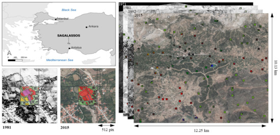
Figure 1.
(top-left) The Sagalassos archaeological site located in the southwest of Turkey; (right) the study area under consideration with indication of the sample locations; (bottom-left) example of an annotated patch at the same geographical location on the 1981 and 2015 orthophoto.
The original orthophotos were provided by the government of Turkey (in 8bit ECW format) and came without any form of metadata. Their resolution varies between px² (1992) and px² (2015), corresponding to a ground sampling distance (GSD) between 0.84 m and 0.30 m, respectively (Table 2). While the 2015 orthophoto is a three-channelled RGB image, the more historical orthophotos are only single channelled images, which we assume to be panchromatic (PAN) in the visible spectrum. However, we have no actual certainty on this. Furthermore, although the four orthophotos all capture the same spatial area, they differ greatly in their digital number (DN) distribution (Figure 2). This may be due to differences in light conditions, differences in time of the year, or differences in the use of camera equipment at the time of acquisition. The latter strongly increases the difficulty for both human and computer aided image interpretation.
Table 2.
Properties of the Sagalassos dataset.
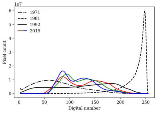
Figure 2.
Digital number distribution of the four orthophotos (after upsampling to the resolution of the 2015 image).
The procedure to construct our manually annotated land cover training data can be summarized as follows: First, we identified 14 mutually exclusive and exhaustive LULC classes. The decision in classes was based on a visual survey of the imagery, terrain knowledge, and requests for use in later research. An overview and description of all classes is given in Table 3. Thereafter, all orthophotos were upsampled to match the resolution of the 2015 image to ensure equal spatial coverage for an equal number of pixels. Images were upsampled instead of downsampled to not lose any information of the 2015 image. Next, a (vector) sample grid of px² ( m²) was overlaid on the study area (Figure 1, bottom-left). A gridsize of 512² px² was chosen because it is the patch input size used in our FCN semantic segmentation model. Subsequently, 100 sampling points were generated using a latin hypercube sampling scheme to guarantee spatial coverage over the study area while remaining statistically substantiated (patches Figure 1, right), and to account for intraclass spectral variability caused by both intrinsic class-appearance variability and spectral variability originating from the merging of multiple aerial photos with varying spectral characteristics to obtain an orthophoto. All grid-plots intersected by a sampling point where then fully manually annotated by drawing non-intersecting polygons and assigning a class-id (Table 3) using the open-source software QGIS (Figure 1, left-bottom). In addition, 15 extra self-chosen plots were selected and annotated to guarantee a minimal coverage for all classes. The above was repeated for all years with the same plots to obtain a dataset suitable for land cover change analysis. Lastly, the polygon layers (shapefile format) were converted to 8-bit geotiff rasters with the same resolution and spatial extent as the orthophotos. Examples of our dataset can be found in Supplementary Figure S1.
Table 3.
Overview and description of the 14 identified land cover classes in the Sagalassos dataset.
Labelling all 115 patches for a single orthophoto took around 3 days of manual work. With a GSD of 0.3 m, the total annotated area for each orthophoto equals to km², or only 2.2% of the total study area. The latter again stresses the need for automation. The distribution of both the patch occurrence and pixel occurrence for each of the 14 classes for the 2015 and 1981 annotated land cover data are visualized in Figure 3. The strong class–imbalance, and the discrepancy between the pixel-count and patch-count distribution is noteworthy. Furthermore, note that the high patch-count of no info(class-id zero) happens (i) because of manual misalignment of polygons, or (ii) because only pixels with their centres within the polygon are assigned the polygon-class when rasterizing. As such, the pixel count of zero-valued pixels is low, but as some pixels occur in each patch, their patch count can be high.
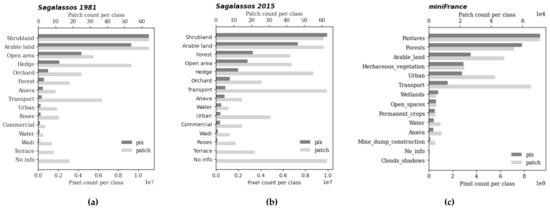
Figure 3.
Distribution of both the pixel and patch count over the different land cover classes for (a) the Sagalassos 2015, (b) the Sagalassos 1981 and (c) the MiniFrance annotation data.
2.2. MiniFrance
Aside from our novel Sagalassos dataset, this research also utilizes the publicly available MiniFrance (MF) dataset [71]. The MF-dataset consists of VHR aerial orthophotos over different cities and regions in France (provided by IGN France), and corresponding Urban Atlas 2012 land cover labels at the second hierarchical level (Table 1). Because MF was introduced to encourage semi-supervised learning strategies for land cover classification and analysis, annotations are only available for a subset of the orthophotos. However, this study only considers the subset which includes land cover annotations. Hence, when referencing MiniFrance, we here refer to the labelled subset of the dataset.
In total, the MF-labelled subset consists of 409 RGB orthophotos (8-bit JPEG 2000 compressed tif format) of dimensions px² and 0.5 m GSD, corresponding to an aerial coverage of roughly 10,225 km². The imagery covers both urban and rural scenes over the counties Nice and Nantes/Saint Nazaire between 2012 and 2014. The land cover labels are provided as rasterized Urban Atlas tiles with equal size and resolution as the orthophotos. Each pixel is integer encoded as one of the 13 occurring classes: urban fabric, transport units, mine/dump/construction, artificial non-agricultural vegetated areas, arable land (annual crops), permanent crops, pastures, forests, herbaceous vegetation associations, open spaces with little or no vegetation, wetlands, water, clouds and shadows. The annotations have a minimum mapping unit (MMU) of 0.25 ha in urban area and 1 ha in rural area [78]. Examples can be found in Supplementary Figure S2.
For this study, we further clipped all 409 orthophotos to patches of px². Clipping was carried out with a stride slightly smaller than 512, such that the boarder of a patch at the edge of an orthophoto fell in line with the boarder of the orthophoto, ensuring maximal use of the data while having minimal overlap. Furthermore, patches were discarded if more than 1% of the patch was unlabeled. This led to a total of 117,832 image–annotation pairs. Figure 3c gives the resulting pixel and patch distribution over the different classes for the MF-dataset.
3. Experiments
3.1. Spatio-Temporal Transfer Learning
As stated in the introduction, we investigate the added value of domain transfer techniques for LULC mapping of historical EO imagery. To this end, we distinguish two types of transfer learning: temporal and spatial. We here define temporal transfer learning as the use of training data of the same study area but of a different moment in time. In this case, the appearance of the imagery may vary due to differences in atmospheric conditions or sensor equipment at the time of acquisition, or due to actual changes of LULC, but the larger part of the spatial features/information remains similar. On the other hand, by spatial transfer learning, we mean the use of training data of a different geographic location. Of course, additional external training data can be both spatially and temporally distinct from one’s own dataset.
To quantify the influence of these two types of transfer learning, we test different training procedures of a multiclass FCN semantic segmentation model. The aim is to obtain a land cover map from a first (monochromatic) historical orthophoto (HIST) with annotations available for a second orthophoto of the same region but without annotations available for the first orthophoto. Therefore, the experimental setup is the following: the 115 image-annotation patches of the 2015 RGB orthophoto in the Sagalassos dataset (SAG2015) serve as training set, while the 115 patches of the 1981 historical orthophoto (SAG1981) serve as test set. Data of 2015 are chosen for training because manual land cover labelling is usually easier on a higher resolution RGB image than a lower resolution greyscale image (Table 2). The 1981 data are chosen for testing since it seemed to have the most challenging DN-distribution (Figure 2). The different steps in the training procedure can now be summarized as: (i) perform or learn an I2I translation from SAG2015 to SAG1981 (i.e., temporal transfer learning), (ii) optionally pretrain the model using either a classical computer vision dataset or a LULC-EO-dataset (i.e., spatial transfer learning), and (iii) fine-tune or train the model using the RGB → HIST mapped 2015 images and their corresponding LULC-annotations (Figure 4).
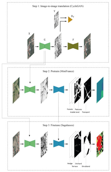
Figure 4.
Training procedure for semantic segmentation of historical orthophotos partitioned into different possible steps. Step 1: image-to-image translation using CycleGAN. X = RGB image domain (Sagalassos 2015 or MiniFrance), Y = historical image domain (Sagalassos 1981), G, F = generators, D = discriminator. Step 2: Pretrain the semantic segmentation encoder–decoder model (blue) on the large RGB—multiclass LULC dataset MiniFrance after manual conversion to greyscale or using the mapping function G. Step 3: fine-tune on Sagalassos 2015 after conversion to ‘historical’ using the mapping function G. The encoder–decoder outputs a probability map for each class, which are subsequently converted into a final land cover map (examples are random and do not match the input).
3.1.1. Temporal Transfer Learning: Image to Image Translation
Performing the mapping from the SAG2015 to the SAG1981 domain can be considered as an I2I translation problem. In addition, it can also be classified as temporal transfer learning since the geographical region under consideration is the same, but the time of acquisition is different for the two orthophotos. Two approaches can be considered here. First, the I2I translation can be performed manually. Usually, for RGB to greyscale mapping, this is the standard option. However, in the case of historical orthophotos, this mapping may not be straightforward because of potential spectral noise, blur, distortions, camera lens marks, spatially depended brightness variations, or dust on the scanner when digitizing the aerial images [4]. Moreover, for the Sagalassos historical orthophotos, we do not have actual certainty regarding their spectral band(s). Therefore, a second approach is to use a model capable of learning a mapping function between these two domains. Hereby, two constraints apply to this model: (i) spatial information must be preserved throughout translation, and (ii) no perfectly paired images are available for training due to potential LULC changes between two images. In computer vision literature, most paradigms that have recently been proposed to tackle the above task are based on conditional generative adversarial networks (GAN) [79]. One such popular GAN architecture is the widely cited CycleGAN [51]. A more detailed description and implementation specifics of CycleGAN are given in Section 3.2.1.
3.1.2. Spatial Transfer Learning: Pretraining
Pretraining CNNs on larger datasets, even datasets from a different domain than the one considered, has in many cases been shown to increase model accuracy while decreasing training time [47]. Therefore, we here experiment with using two different datasets for pretraining our model and compare this versus using no pretraining: one classical natural image dataset, namely ImageNet [37], and one large multiclass LULC-EO dataset, namely MiniFrance. The MF-dataset was chosen because, out of all datasets listed in Table 1, it shows the most similarities with our Sagalassos dataset, i.e., it is continuously annotated (instead of one label per patch), multiclass with similar LUCL classes, has a similar resolution, the same spectral bands (RGB), and comparable landscape characteristics, e.g., urban, rural and mountainous regions. One main difference is that annotations are of a much courser resolution in the MF-dataset than in the Sagalassos dataset. Moreover, after visual inspection, labelling seems to be far from perfect for MF. Nonetheless, we hypothesise that pretraining with MF will help the model to learn robust features and higher-level semantics characteristic to EO-data. However, we still chose to fine-tune the whole model with the aim to segment the semantic classes at a more fine-grained level. Additionally, we also test the case of only fine-tuning the final classification layer of the model. Furthermore, we explore the possibility of applying the I2I translation as explained in the previous section to the MF dataset, to obtain a large mimicked historical EO dataset with the characteristics of the 1981 Sagalassos orthophoto. For the latter, either the mapping function learned between SAG2015 and SAG1981 can be employed, or a separate second mapping function between MF and SAG1981 can be learned.
3.2. Neural Network Models
3.2.1. Image to Image
This section briefly explains the concepts and implementation details of the I2I translation model CycleGAN, which we utilize in this study to learn a mapping function between more recent RGB EO-imagery and historical monochromatic EO-imagery. Contrary to I2I translations models that require paired observations for training such as pix2pix [80], CycleGAN can learn a mapping function between two image domains X and Y based only on an unpaired set of observations with size N. The aim is to optimize this function such that images generated by are indistinguishable from the images of Y, while at the same time learning a second inverse mapping function which is optimized to enforce (Figure 4). Similarly, the images Y can be cycled such that is indistinguishable from X and . The above constraints can be imposed on the generators G and F by using a combination of three losses:
where is the adversarial loss, the cycle-consistency loss [54], the identity loss, and and parameters to control the relative contribution of the cycle and identity loss to the total loss, respectively. For the generator F, the losses are further defined as:
which are estimated as the mean absolute error (MAE) between observations x and their reconstruction and identity mapping, respectively, and
which is estimated as the mean squared error (MSE) of . Here, is called the discriminator for domain X, which is a separate CNN that takes as input a generated image together with a true image (e.g., ) and outputs a (number of) value(s) between zero and one, where one represents full certainty of and x belonging to the same domain, and zero the opposite. The two discriminators and are in turn optimized with their own loss:
In case of the , this becomes:
where is estimated as the MSE of one minus the discriminator output of a real example, and is estimated as the MSE of the discriminator output of a fake example. The definitions for and are analogous. In other words, the discriminators try to classify real examples as True, and fake examples as False, while the generators try to fool the discriminator by generating fake examples indistinguishable from the true examples. During training, the four losses are (, , , ) are optimized conjointly in a zero-sum game.
The CycleGAN model is implemented using Keras and Tensorflow based on AKNain (2020) [81]. In summary, the architectures of the generators and discriminators are the following. The generators are composed of two downsampling blocks, nine residual blocks, two upsample blocks, and a final convolution layer with tanh activation. The different blocks use reflection padding, instance normalization, and ReLU activation. On the other hand, the discriminators are composed of three downsampling blocks with Leaky ReLU activation.
3.2.2. Semantic Segmentation
We here elaborate on the choices made regarding the multiclass semantic segmentation model. We follow the currently popular strategy of combining a strong performing CNN classifier as an encoder together with a decoder. As such, the main model we use for our experimental setup is a UNet-like architecture with an EfficientNetB5 backbone (UNet-EffB5). The architecture is given in detail in Figure 5. EfficientNets are a family of CNN models proposed by Tan et al. [82], which show state-of-the-art accuracy while being considerably smaller and faster. The models are designed using neural architecture search and subsequent upscaling using a compound coefficient, which uniformly scales all network dimensions depth, width, and resolution. Its central building block is the mobile inverted bottleneck MBConv with squeeze-and-excitation optimization (Figure 5b). EfficientNet variants are available from a base model B0 (5.3 million parameters) up to the largest model B7 (66 million parameters). In this study, we opted for EfficientNetB5 (30 million parameters), as a trade-off between model size and accuracy. The encoder is connected with a decoder which uses transposed convolutions for upsampling and skip connections to concatenate corresponding encoder layers according to the original UNet [33]. The last decoder block is connected to a final classification convolution with softmax activation, which produces K probability maps, with K the number of classes, of equal dimensions as the input image. The final LULC-map in integer format can then be derived by assigning to each pixel the class with the highest probability (= argmax). In addition, we compare the UNet-EffB5 model above to two other state-of-the-art semantic segmentation models: DeepLabV3+ with Xception backbone (output stride 16) [83] and Feature Pyramid Network with EfficientNetB5 backbone (FPN-EffB5) [84]. In this comparison, the three models are all trained from scratch, i.e., they are not pretrained such as in the experimental setup for transfer learning where only UNet-EffB5 is considered. For UNet-EffB5 and FPN-EffB5, the model implementations of Yakubovskiy (2019) [85] were used, for DeepLabV3+, the implementation based on Lu (2020) [86] was used. All models were implemented with Keras (v2.4.0) and Tensorflow (v2.4.1).
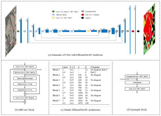
Figure 5.
(a) Overview of the UNet fully convolutional network with EfficientNet-B5 backbone. The horizontal values indicate the number of filters. The vertical values indicate the image height and width (H = W). K equals the number of LULC classes. Detailed schematics are given for the mobile inverted bottleneck with squeeze-and-excitation building block (MBConv) and the upsample building block in pane (b,d), respectively. The filter kernel sizes k × k, and number of filters and for the multiple MBConv blocks are specified in pane (c). BN = batch normalization, ReLU = rectified linear unit, DwConv = depthwise 2D separable convolution (always with stride = 2).
3.3. Model Training and Evaluation
3.3.1. CycleGAN
The CycleGAN model was trained two times: a first time to learn the mapping function SAG2015↔ SAG1981, and a second time to learn the mapping function MF↔ SAG1981. In case of the former, the images of the 2015 and 1981 Sagalassos orthophotos were clipped to non-overlapping patches of px², totalling 4320 patches for each year. Subsequently, the patches were resized to px² (for computational reasons), and rescaled to the [−1, 1] domain. The 1981 monochromatic patches were copied three times and concatenated to itself to match the three-channel shape of the 2015 RGB patches. The pairs of {SAG2015, SAG1981} patches were chosen to remain geographically aligned when fed into the model during training, to encourage I2I translation of structures that remained the same over the two years. For the case MF↔ SAG1981, the procedure was analogous, except that first a 10% random sample out of all patches was taken, resulting in 11,785 patches. These patches were then randomly paired with SAG1981 patches.
In both cases, the model was trained for 50 epochs with the Adam optimizer, a learning rate of and momentum of 0.5, a batch size of 1, random normal kernel and gamma initialization with zero mean and 0.02 standard deviation, and cycle and identity loss contribution of and , respectively. Model weights were saved every 5 epochs, and the result evaluated visually on 0.5% validation patches. Training took approximately 13 h and 35 h using Google Colab Pro (Tesla V100, 16 GB), respectively. For SAG2015↔ SAG1981, the model at epoch 50 was selected, while, for MF↔ SAG1981, the model at epoch 10 was selected.
3.3.2. Segmentation Models
(a) Training loss: The different semantic segmentation models and configurations were trained by minimizing a combination of the dice loss (=F1 loss) and categorical cross entropy (CCE) loss. These losses are calculated as a certain distance between the class probability maps predicted by the model and the one-hot encoded true annotations. The soft dice loss for a certain class c is calculated as one minus twice the intersection over the total sum:
With the predicted class probability for pixel i, , the binary ground truth, N the total number of pixels, p an optional exponential coefficient, and a constant to prevent from zero division. The latter two were set at to stimulate a steeper loss decrease at higher losses and to ensure stability during training, respectively. Contrary to the dice loss, the CCE is calculated per-pixel and is given by:
with K the total number of classes and the pixel-level class weights. These weights are introduced to account for class-imbalance in the training set. The total loss can then be calculated as a weighted average of and :
where is a hyperparameter determining the relative contribution of both losses to the total loss. After a 1D grid-search using the 1971 Sagalassos data, we set (Figure 6). The 1971 Sagalassos data was used because this was the only orthophoto for which annotation data were available at the time. For all configurations, model training was repeated five times, each time with a different 90–10 train–validation split as a trade-off between having sufficient training data and being statistically representative. Train–validation splits were only accepted if all classes were present in both sets. The soft IoU loss (see Equation 12) was also tested as an alternative for the dice loss but did not show an improvement (Figure 6). Furthermore, the total loss was always calculated over the whole batch, and only pixels for which a known ground truth existed were considered, i.e., the class No info was not considered.
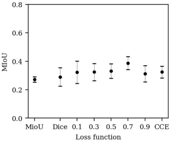
Figure 6.
Mean intersection over union (mIoU) of the 1971 Sagalassos validation set for different loss functions. The numbers on the x-axis represent a weighted average between the dice loss and CCE loss ( in Equation (9)). The average over five runs (± stdev) is shown, except for mIoU loss with only three runs.
(b) Multiclass weighting: Observe that is calculated per class and subsequently averaged, while is calculated per pixel and subsequently averaged. Therefore, in contrast to the CCE, the dice loss is weighted with a second set of class-weights, which we call here patch-level class weights . The usage of two distinct sets of class-weights is supported by the existence of a discrepancy between the probability of pixel-wise class occurrence, which is determined by the object size of the class, and the probability of patch-wise class occurrence, which is determined by the dispersion of the class. This can clearly be seen in Figure 3. We define both class-weight sets inversely proportional to the probability of occurrence, i.e., . If we denote the probability of a randomly selected pixel belonging to a certain class as , and assume the expected probability of for all classes to be uniform, i.e., , then is calculated as:
In words, the pixelwise weight given to a class is the inverse of the observed class-probability versus the expected class-probability. Hence, classes with are down-weighted while classes with are up-weighted. On the other hand, the patchwise class-weights are calculated as:
with being the probability that a certain class occurs in a randomly selected patch. In words, the patch-wise weight given to a class is the inverse of the observed class-probability divided by a normalization factor such that the sum of the weights is one. The rationale is again that classes with high occurrence are down-weighted while classes with low occurrence are up-weighted. In both cases, the class probabilities are estimated as the relative class frequencies, i.e., (Figure 3).
(c) Evaluation metrics: The different experiments were evaluated using the common class-wise mean Intersection over Union (IoU) metric, which for a certain class is calculated as:
Here, in contrast to Equation (7), the model predictions are binary, i.e., they are evaluated after the argmax operator. As such, this is equal to the definition . The final mean IoU (mIoU) is then the average over the different classes: . Additionally, the mean true positive rate (mTPR) was calculated as a second evaluation metric:
3.3.3. MiniFrance Pretraining
The UNet-EffB5 model was trained on the MF-dataset with three different input configurations: a first time with RGB input (MF), a second time with greyscale input (MF), and a third time with historical input (MF). By historical input, we mean the RGB patches that have been converted to historical-looking images using the mapping function learned by CycleGAN and their corresponding original annotations. In all cases, the model was trained on 90% of the data for 10 epochs with the Adam optimizer, a batch size of 2 (maximum that fitted into RAM), a fixed learning rate of 0.0002, and an ImageNet pretrained encoder. The other 10% of the data was used for validation. Apart from scaling images to the 0–1 domain, no pre-processing was conducted. In the case of the greyscale and historical input, the images were copied and concatenated three times to match the three-channel input of the model. Each training run took around 46 h on a NVIDIA RTX 2080.
3.3.4. Sagalassos Training/Fine-Tuning
Different experiments were trained on the Sagalassos data: with or without pretraining on ImageNet (only encoder), MF or MF (full model); using manual RGB to greyscale (historical-looking) mapping (SAG2015) or CycleGAN mapping (SAG2015) as input; and using different FCN architectures. All configurations were trained for 100 epochs with the Adam optimizer, a batch size of 4, and the following learning rate schedule:
With , , and . Furthermore, the original training dataset was augmented by increasing image-context around the annotated patches, i.e., a context of 256 px around the patches was considered, after which patches of the same size () were clipped with a stride of 265 px. As such, one annotated patch results in nine patches (of which one the original), where each of the four subpatches within the larger patch is seen four times from four different angles (Figure 7). Discarding the patches at the edge, this led to 1002 training examples. Additionally, patches were randomly flipped horizontally and/or vertically. For the case of manual RGB → HIST mapping (SAG2015), additional random brightness shifts and random noise were added to visually mimic the characteristics of the SAG1981hist images. The models were trained on of the data and validated on the other . It was ensured that all classes were present in both the train and validation set. Training was performed using Google Colab Pro (Tesla V100, 16 GB) and took around 3.6 h.
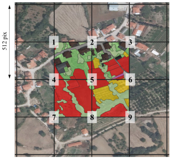
Figure 7.
Illustration of data augmentation by using additional image-context. One annotated patch now becomes nine patches (numbers are located in the centre of a patch).
3.4. Inference and Post-Processing
3.4.1. Inference
After training, the model was deployed to derive a LULC map for the whole 1981 Sagalassos orthophoto. The most straightforward way to achieve this is by sliding a window of 512 × 512 px² (= model input size) over the orthophoto with stride 512 px and predicting the LULC for each patch. However, a drawback of this procedure is that the edge-pixels of a patch have a considerable chance of being predicted differently than the edge-pixels of an adjacent patch due to reduced context information at the edges, hence resulting in an undesired raster-like effect over the predicted LULC map. To overcome the latter, we use a stride smaller than the patch size during inference such that each pixel is seen multiple times and predicted with different context. The predictions can then be aggregated by, among others, averaging the probabilities or maintaining only the prediction with the highest probability (remark that this aggregation occurs prior to the argmax operator). However, there is a trade-off with the latter solution: when decreasing the stride, the inference time will increase proportionally. For example, if we wish to predict all pixels four times (stride = 256), inference time will take four times as long. Therefore, in this study, we quantify the prediction accuracy gain when decreasing the inference-stride and compare this to the inference time increase.
3.4.2. Post-Processing
As a final post-processing step, we also tested the effect of combining the LULC map outputted by the FCN model with an unsupervised segmentation method. The rationale is to segment the original orthophoto into superpixels, and subsequently assign to each superpixel the most occurring class-id from the corresponding LULC map within the superpixel. The aim of the latter is to ameliorate boundary delineation between semantic objects and to establish a certain MMU. In this study, we opted for the popular simple linear iterative clustering (SLIC) method [87] implemented by van der Walt et al. (2014) [88], which in our case simply performs k-mean clustering in the 3D image intensity-location space, making SLIC very efficient. The algorithm has two main parameters: the compactness, which trades off colour-similarity and proximity, and the desired number of approximately equally-sized superpixels. The two parameters were set at 0.05 and 1000, respectively. The high number of centres ensured oversegmentation, such that the obtained super-pixels were not larger than the semantic objects. Furthermore, for better efficiency, the segmentation was run patch-wise instead of using the complete orthophoto as input. A patch size slightly smaller than the inference patch size was used such that also superpixels were generated which overlaid the inference-caused edge artifacts.
4. Results
4.1. Image to Image Translation
Example results of the I2I translation between SAG2015 and SAG1981 using the trained CycleGAN model are given in Figure 8. Translation and reconstruction are shown in both directions. Similarly structured examples for the learned MF↔ SAG1981 mapping are given in Supplementary Figure S3. From visual inspection, the CycleGAN model seems adequately capable of learning the RGB → HIST mapping function. Furthermore, the spatial/textural information is well preserved throughout RGB → RGB reconstruction; however, some colour information is lost as the model seems to have the tendency of leaning towards colour shades with a high occurrence in the training set. For example, observe the orange house roofs that did not make it through reconstruction (Figure 8).
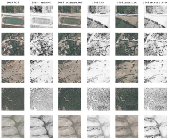
Figure 8.
Validation examples of image-to-image translation between the Sagalassos 2015 and 1981 orthophoto domains using CycleGAN. Corresponding image patches are of the same geographical location.
Although the model with weights trained for 50 epochs was selected, an acceptable translation was already learned after very few epochs. Moreover, in the case of MF↔ SAG1981, training even became unstable after a higher number of epochs (Supplementary Figure S4). This seems to indicate that having a training dataset which includes some degree of approximately pairwise examples is still beneficial for training stability of CycleGAN. Nonetheless, the observation that the automated translation step can be learned by relatively few epochs signifies that it still could prove valuable in more time-constraint projects. In addition, while in this study, we learned a separate mapping function for MF↔ SAG1981 translation, the mapping function learned on SAG2015↔ SAG1981 could have also been used for this. Although this led to rather similar translation but inferior reconstruction results (Supplementary Figure S5), it would eliminate the need to train a second mapping function, thus also reducing computation time.
4.2. Transfer Learning
Table 4 summarizes the results of the different experiments related to transfer learning. Several conclusions can be drawn. First, all configurations score considerably higher on the validation than on the test set. The main reasons for this are that (i) parts of the validation set were also present in the training set due to the data augmentation technique used (Section 3.3.4), thus probably leading to an overestimation, (ii) the validation and test set were to a large extent labelled by different annotators, thus resulting in different annotation choices, (iii) spatial features are present in the landscape of 1981 which are not present in 2015, or (iv) there is an imperfect mapping between 2015 and 1981. Second, the experiments demonstrate the added value of pretraining. Moreover, the added value increases when using a dataset for pretraining closer to the desired image domain. More specifically, Figure 9 shows that pretraining on the EO dataset MiniFrance results in higher segmentation scores and faster convergence during training than pretraining on the natural image dataset ImageNet, even though MiniFrance is far from perfectly annotated and the models trained on MiniFrance do not necessarily exhibit maximal accuracy (Table 5). In particular, the mIoU increases with 13.0% when comparing no pretraining with MF pretraining, both with SAG15 fine-tuning (Table 4). Third, using a learned mapping function RGB → HIST gives a substantial gain compared to manually mimicking the conversion. That is, the mIoU increases with 27.2% when comparing SAG15 with SAG15 fine-tuning, both with ImageNet pretraining. Hence, the latter two conclusions prove the added value of our proposed combination of spatial and temporal transfer learning methodology. Lastly, the highest validation mIoU is attained when combining initial pretraining on the CycleGAN mapped MiniFrance dataset (MF) with subsequent fine-tuning of all layers on the CycleGAN mapped Sagalassos 2015 dataset (SAG15). However, the highest test mIoU is attained when pretraining on MF, or when only fine-tuning the final classification/convolutional layer (f.c.). As such, a higher validation score in this case does not per se correspond to a higher test score, as highlighted previously.
Table 4.
Summary of the multiclass semantic segmentation results on the Sagalassos (SAG) 2015 validation set and 1981 test set. All experiments use the UNet-EffB5 architecture. ‘-grey’ means manual RGB → HIST conversion, ‘-hist’ (=historical) means learned mapping with CycleGAN.
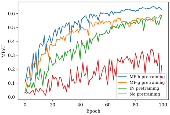
Figure 9.
Mean intersection over union (mIoU) of the 2015 validation set (CycleGAN translated) during training when using no pretraining, ImageNet (IN) pretraining, MiniFrance (MF) greyscale (-g) or historical-like (-h, CycleGAN translated) pretraining.
Table 5.
Summary of semantic segmentation results using UNet-EffB5 on the MiniFrance (MF) validation set using RGB, greyscale or historical-like (CycleGAN translated) input.
Table 6 further compares UNet-EffB5 versus the FPN-EffB5 and DeepLabV3+ architectures (all trained from scratch). UNet-EffB5 yields the highest scores on the validation set but ranks last on the test set, thus seemingly having lower capacity to generalize from the validation to the test set. Hence, for future research, it may be interesting to apply the spatio-temporal transfer learning methodology using different CNN architectures.
Table 6.
Summary of semantic segmentation results using UNet-EffB5 on the MiniFrance (MF) validation set using RGB, greyscale or historical-like (CycleGAN translated) input.
4.3. Semantic Segmentation
The results presented here all build on the best performing model from the previous section, i.e., initial MF pretraining and subsequent SAG2015 fine-tuning of the final classification layer (Table 4). Example results and the confusion matrix of the SAG2015 validation set are given in Supplementary Figures S6 and S7, respectively.
To obtain the final LULC map for the complete 1981 orthophoto, various inference strides were tested as summarized in Table 7. Several observations can be made. First, decreasing the inference stride does not seem to significantly impact the test mIoU; however, visually it drastically improves the quality of the LULC map. Figure 10 shows that the raster-like appearance of the LULC map caused by using no overlap fades when using overlap, making the map much smoother across the patch edges. Second, assigning each pixel the class with the highest average probability over the multiple overlapping predictions yields a better segmentation score than assigning each pixel the class with the overall highest probability. Third, using the additional SLIC super-pixel post processing step does not improve the segmentation score. Moreover, qualitatively it does not seem to be of much added value for boundary delineation (Figure 10). Nonetheless, SLIC reduces noisiness of the LULC map and can prove useful for establishing a certain MMU (Figure 10).
Table 7.
Summary of semantic segmentation results on the Sagalassos 1981 test set for various inference strides relative to the patch size with either average (avg) or maximum (max) aggregation, and for the combination with SLIC post processing.
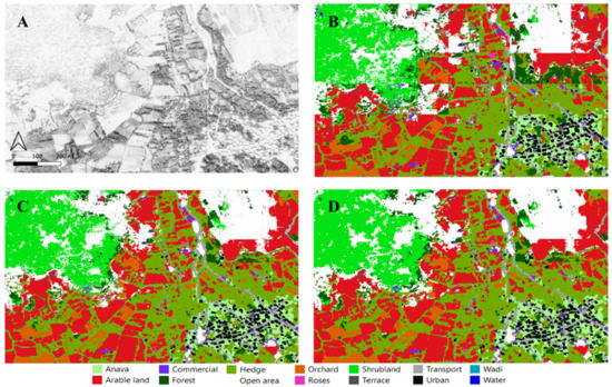
Figure 10.
(A) Part of the Sagalassos 1981 orthophoto, with (B) corresponding predicted LULC map using no overlap during inference, (C) using a relative stride of 1/4th of the patch size during inference, and (D) combining the latter with SLIC post processing.
Hence, the final LULC map is derived by using the best performing model with 1/4 inference stride and SLIC post-processing, having a mIoU = 31.1%, mTPR = 46.1%, and an overall accuracy of 69%. Mapping the entire study area when running inference with no overlap took around 7.3 min, or approximately 0.28 km2 · s−1 at 0.3 m GSD (Table 6). Consequently, mapping with relative inference stride of 1/4 took about 2 h. The final entire predicted 1981 LULC map is depicted in Figure 11.
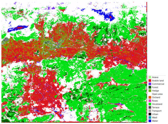
Figure 11.
Predicted LULC map for the entire 1981 Sagalassos orthophoto based on the 2015 training data (MiniFrance-hist pretrained + SAG2015-hist fine-tuned).
Figure 12 further provides the pixel-wise confusion matrix between the ground truth and predicted LULC classes. Ideally, all diagonal elements in the confusion matrix approximate 100%, indicating that all pixels are correctly predicted as their true LULC class. Deviation from this diagonal thus learns which classes are mutually confused and are under or over predicted. Note, however, that it is not necessarily desired to reach exactly 100% because the ground truth annotations will contain errors as well. Hence, a combination with qualitative inspection of the LULC map is needed. It can be seen that the semantic segmentation model strongly overfits on the class open area, moderately overfits on the classes hedge and arable land, and slightly overfits on the classes transport and shrubland, as their columnwise sum is larger than 100%. This is also reflected in Figure 13, which shows some example predictions for the 1981 test set with corresponding ground truth. Consequently, the other classes are underpredicted. More specifically, the model fully misclassifies wadi and water mainly as open area (see for example top of Figure 11), and further has difficulty with recognising—in descending order—roses, terrace, anava and commercial. Except foranava, the latter classes all had the least training examples (Figure 3), which we believe to be the principal cause for their lower class accuracies. We do not consider it to be attributable to a poor handling of the class-imbalance in the training set, as for example the class urban, which albeit also having few training examples, still shows a high class TPR, likely because of its rather low intra-class variability. As such, we believe the weighting scheme incorporated into the loss function to be effective, but it is the lack of training examples for classes with high intraclass variability or low inter-class variability that causes the low class-accuracies. Lastly, visual inspection of the LULC predictions further learns that the model struggles with areas of very low contrast, especially on both ends of the spectral spectrum, and with areas which are also difficult to discriminate through human interpretation.
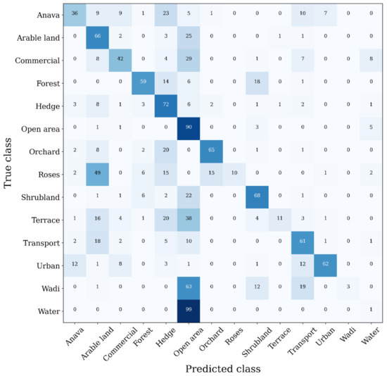
Figure 12.
Confusion matrix of the predicted vs. the true LULC classes for the Sagalassos 1981 test set. Values are given as percentages over the true class.
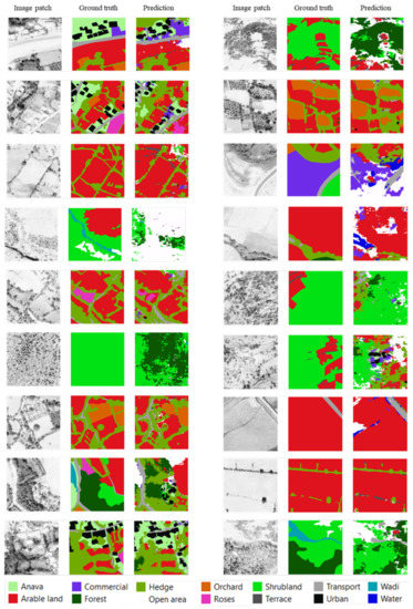
Figure 13.
Example image patches of the Sagalassos 1981 test set with corresponding LULC ground truth and prediction.
5. Discussion
We further discuss our results and present an outlook on future research perspectives and opportunities. Firstly, improvements could be made regarding the semantic segmentation model through evaluation of other existing models in literature, either specifically tailored to the EO problem at hand or transferred from another domain. For instance, some works investigate the potential of graph-CNNs which seems promising for hierarchical segmentations [89], while other studies intend to find architectures applicable in more resource constraint settings [90]. In addition, a popular strategy is to obtain final predictions through combination of an ensemble of high-performing segmentation models [91]. In addition, with increasing availability of multi-temporal EO data, a growing body of research is dedicated to change detection for which specific DL paradigms have been developed such multitask or convolutional siamese networks [72,92,93], which may be a promising direction particularly for historical land cover mapping. Furthermore, a strategy to better deal with multiclass problems could be to use separate optimized models for each target LULC class and collect class-specific open-source data for pretraining, however, when dealing with a high number of classes, this would be extremely demanding. Next, although this work used a SLIC post-processing step, deep learning based semantic segmentation models have arguably reached a state where they either incorporated the post-processing rationale into the model structure (e.g., border refinement, conditional random fields, …) or reached state-of-the-art performances without needing the additional step, hence rendering post processing obsolete.
While a lot of endeavour aims at improving DL architectures, significant performance gains can also be achieved by leveraging transfer learning and domain adaptation, as signified in this study. On the level of pretraining, the release of new large-scale open-source HR or VHR EO datasets with accurate multiclass LULC annotations will likely have the most substantial impact on driving research forward and closing the gap between research and real-world applications. In this light, it may be interesting to investigate the impact of the accuracy of ground truth LULC labels, by, for example, comparing pretraining on the MiniFrance dataset with pretraining on the Chesapeake land cover Dataset which has more reliable high-resolution labels (Table 1) [18]. On the level of domain adaptation, we expect a significant increase in studies exploring I2I translation within the EO domain. Improvements are possible in terms of DL models—chiefly GANs—or general methodology. As an example, for the former, the recent contrastive-unpaired-translation (CUT) model could substitute CycleGAN as it enables faster and more memory-efficient training [94]. Methodology-wise, there is active work on considering GANs for semantic segmentation—as semantic segmentation is in essence an I2I problem—thereby integrating the workflow of domain adaptation and semantic segmentation [57,95]. Furthermore, Tasar et al. [58] propose an interesting approach for multi-source domain adaptation by data standardization.
Besides the model architecture and transfer learning methodology, remarks can be made regarding the dataset construction. A difficult question to answer is ‘how much training data are needed?’ One approach is to follow an ‘active learning’ scheme, by alternating between training the model and manually annotating additional data there where needed. Plotting the model accuracy versus the fraction/quantity of training data can then inform when the accuracy reaches a plateau. It would be interesting to make such a plot for each target class. Additionally, to reduce the problem complexity—if desired—the number of classes could be decreased or the MMU could be increased to derive a less fine grained but smoother LULC map. Next, although the Sagalassos dataset was constructed at GSD = 0.3 m, patch size = px² and 115 patches, alternatives are to work with fewer patches but larger patch sizes. Therefore, exploring best practices in terms of LULC sampling strategy and its effect on the FCN performance could prove valuable research. Furthermore, it can be worthwhile to examine the effect of performing semantic segmentation at a lower resolution (e.g., GSD = 1.0 m), causing the loss of fine-grained information but in return increasing the geographic context and thus also decreasing computational demand. Another potential alteration to the training data are to erode the LULC annotation polygons to cope with the fact that manual annotations at class borders are mostly imperfect. Furthermore, in addition to modifications regarding LULC annotation creation, future work can explore the added value of including an open-source DEM, which, for example, could help in distinguishing classes based on altitude (e.g., higher up the mountain is commonly open area while the valleys are commonly arable land). Of course, if no historical DEM is available, the DEM should be assumed constant throughout time. Lastly, the quality of the final LULC map may be improved by creating some manual annotations for the historical orthophoto to be classified, in particular for the classes with lower segmentation scores, and fine-tuning a second time.
Albeit the seemingly endless list of research opportunities, we first intend to apply our proposed methodology to extract LULC maps for the remaining historical orthophotos in the Sagalassos dataset (1971, 1992). Moreover, our methodology can be applied when new historical images/orthophotos become available for which there are no annotation data.
6. Conclusions
This work introduces a novel methodology for automated extraction of multiclass LULC maps from historical monochromatic orthophotos under the absence of direct ground truth annotations. The methodology builds on recent evolutions in deep learning, leveraging both domain adaptation and transfer learning, which—in the context of EO—we jointly introduce as ‘spatio-temporal transfer learning’. In summary, it consists of three main steps: (i) train an image-to-image translation network for domain adaptation, (ii) pretrain a semantic segmentation model on a translated large public dataset using the I2I function, and (iii) fine-tune using a small translated custom dataset using the I2I function.
The methodology is tested on a new custom dataset: the ‘Sagalassos historical land cover dataset’, which consists of three historical orthophotos (1971, 1981, 1992) and one recent RGB orthophoto (2015) of VHR (0.3 m GSD) all capturing the same greater area around Sagalassos archaeological site (Turkey) and corresponding manually created annotation (2.7 km² per orthophoto) distinguishing 14 challenging LULC classes. Although this study considers the 2015 image with ground truth as training set and the 1981 image with ground truth as test set, the Sagalassos dataset can be used for other future research on semantic segmentation of historical EO or multi-temporal change detection paradigms. Furthermore, this study provides a comprehensive overview of open source annotated EO datasets for multiclass semantic segmentation. For our scope, the MiniFrance dataset proved the most suitable for use as pretraining dataset. However, new large-scale open-source datasets with higher quality labels may become available in the future.
The DL models used in this work are CycleGAN for I2I translation, and UNet with EfficientNetB5 backbone for multiclass semantic segmentation. Both models proved successful for their tasks. Nonetheless, in the future, they may be substituted by more domain tailored models or less resource consuming models allowing for real-time applications.
Our results further indicate that the proposed methodology is effective, increasing the mIoU by 27.2% when using the learned I2I mapping function compared to manual I2I mapping, and by 13.0% when using domain pretraining compared to using no pretraining. Additional improvement will probably be most efficiently obtained by increasing the number of training examples for classes with low occurrence. Furthermore, transferring weights from a model pretrained on a large dataset closer to the target domain is preferred. As such, we believe that, in the near future, DL for EO will solely leverage transfer learning from within the domain, as quantity, diversity and accessibility of EO-datasets will increase. GAN-based I2I translation techniques can hereby effectively help in constructing datasets for a target domain when the mapping function between a source domain (with annotations) and target domain (without annotations) is not straightforward.
Post processing by casting a majority vote over superpixels generated by the unsupervised SLIC algorithm proved useful to install a MMU and make slightly smoother maps; however, it is not convincingly worth the additional computation. In contrast, decreasing the stride during inference to make aggregated predictions for the complete orthophoto resulted in significantly higher quality and seems key for geographical continuity of the LULC maps.
Using our methodology, we generated the first historical LULC map for the greater area around the Sagalassos archaeological site for the year 1981. Analogously, we plan to compute LULC maps for the 1971, 1992 and 2015 orthophotos, which will be instrumental to support future studies focussing on long-term environmental and agro-social-economical transformations in the Sagalassos region.
Supplementary Materials
The following supporting information can be downloaded at: https://www.mdpi.com/article/10.3390/rs14235911/s1. Figure S1: Examples of the Sagalassos dataset; Figure S2: Examples of the MiniFrance dataset (tile dimensions are 10,000 × 10,000 px²); Figure S3: Validation examples of image-to-image translation between the MiniFrance (RGB) and Sagalassos 1981 historical orthophoto (panchromatic, PAN) domains using CycleGAN trained for 10 epochs; Figure S4: Validation examples of image-to-image translation between the MiniFrance (RGB) and Sagalassos 1981 historical orthophoto (panchromatic, PAN) domains using CycleGAN trained for 50 epochs; Figure S5: Examples of image-to-image translation between the MiniFrance (RGB) and Sagalassos 1981 historical orthophoto (panchromatic, PAN) domains using the mapping function learned between the Sagalassos 2015 and 1981 domains using CycleGAN; Figure S6: Example image patches of the Sagalassos 2015 validation set (CycleGAN translated) with corresponding LULC ground truth and prediction. The black regions in the ground truth are due to our data augmentation technique (Section 3.3.4); Figure S7: Confusion matrix for the Sagalassos 2015 validation set using the UNet-EffB5 architecture, MiniFrance-hist pretraining and SAG15-hist fin. conv. fine-tuning. Values sum to 100% over the true label.; Figure S8: Confusion matrix for the MiniFrance-historical (CycleGAN translated) dataset. Values sum to one over the true label. Nan-values are because these two classes do not appear in the dataset despite being mentioned in the dataset description.
Author Contributions
Conceptualization and validation: W.A.J.V.d.B., T.G. and M.L.; methodology: W.A.J.V.d.B. and T.G.; data curation: W.A.J.V.d.B. and M.L.; software, formal analysis, investigation, visualization and writing—original draft preparation: W.A.J.V.d.B.; resources, writing—review and editing, supervision, project administration and funding acquisition: T.G. and M.L. All authors have read and agreed to the published version of the manuscript.
Funding
This research was partially funded by the Sagalassos Archaeological Research Project, via Internal Funds KU Leuven C14/17/025.
Conflicts of Interest
The authors declare no conflict of interest.
Abbreviations
The following abbreviations are used in this manuscript:
| CCE | Categorical Cross Entropy |
| CNN | Convolutional Neural Network |
| DL | Deep Learning |
| DN | Digital Number |
| EO | Earth Observation |
| FCN | Fully Convolutional Network |
| FPN | Feature Pyramid Network |
| GAN | Generative Adversarial Network |
| GEOBIA | Geographical Object Based Image Analysis |
| GSD | Ground Sampling Distance |
| HIST | Historical-like monochromatic image |
| HR | High Resolution |
| I2I | Image-to-Image |
| LULC | Land-Use/Land-Cover |
| MAE | Mean Absolute Error |
| mTPR | mean True Positive Rate |
| MF | MiniFrance |
| mIoU | Mean Intersection over Union |
| MMU | Minimum Mapping Unit |
| MSE | Mean Squared Error |
| OA | Overall Accuracy |
| PAN | Panchromatic |
| ReLU | Rectified Linear Unit |
| RGB | Red, Green, Blue optical image |
| RS | Remote Sensing |
| SAG | Sagalassos |
| SLIC | Simple Linear Iterative Clustering |
| UDA | Unsupervised Domain Adaptation |
| UNet-EffB5 | UNet with EfficientNet-B5 backbone |
| VHR | Very High Resolution |
References
- Gómez, C.; White, J.C.; Wulder, M.A. Optical remotely sensed time series data for land cover classification: A review. ISPRS J. Photogramm. Remote. Sens. 2016, 116, 55–72. [Google Scholar] [CrossRef]
- Thyagharajan, K.K.; Vignesh, T. Soft Computing Techniques for Land Use and Land Cover Monitoring with Multispectral Remote Sensing Images: A Review. Arch. Comput. Methods Eng. 2017, 26, 275–301. [Google Scholar] [CrossRef]
- Hoeser, T.; Bachofer, F.; Kuenzer, C. Object Detection and Image Segmentation with Deep Learning on Earth Observation Data: A Review—Part II: Applications. Remote Sens. 2020, 12, 3053. [Google Scholar] [CrossRef]
- Mboga, N.; D’Aronco, S.; Grippa, T.; Pelletier, C.; Georganos, S.; Vanhuysse, S.; Wolff, E.; Smets, B.; Dewitte, O.; Lennert, M.; et al. Domain Adaptation for Semantic Segmentation of Historical Panchromatic Orthomosaics in Central Africa. ISPRS Int. J. Geo-Inf. 2021, 10, 523. [Google Scholar] [CrossRef]
- Mboga, N.; Grippa, T.; Georganos, S.; Vanhuysse, S.; Smets, B.; Dewitte, O.; Wolff, E.; Lennert, M. Fully convolutional networks for land cover classification from historical panchromatic aerial photographs. ISPRS J. Photogramm. Remote. Sens. 2020, 167, 385–395. [Google Scholar] [CrossRef]
- Ratajczak, R.; Crispim-Junior, C.F.; Faure, E.; Fervers, B.; Tougne, L. Automatic Land Cover Reconstruction from Historical Aerial Images: An Evaluation of Features Extraction and Classification Algorithms. IEEE Trans. Image Process. 2019, 28, 3357–3371. [Google Scholar] [CrossRef]
- Deshpande, P.; Belwalkar, A.; Dikshit, O.; Tripathi, S. Historical land cover classification from CORONA imagery using convolutional neural networks and geometric moments. Int. J. Remote. Sens. 2021, 42, 5144–5171. [Google Scholar] [CrossRef]
- Ettehadi Osgouei, P.; Sertel, E.; Kabadayı, M.E. Integrated usage of historical geospatial data and modern satellite images reveal long-term land use/cover changes in Bursa/Turkey, 1858–2020. Sci. Rep. 2022, 12, 9077. [Google Scholar] [CrossRef]
- Morgan, J.L.; Gergel, S.E.; Coops, N.C. Aerial Photography: A Rapidly Evolving Tool for Ecological Management. BioScience 2010, 60, 47–59. [Google Scholar] [CrossRef]
- Pinto, A.T.; Gonçalves, J.A.; Beja, P.; Pradinho Honrado, J. From Archived Historical Aerial Imagery to Informative Orthophotos: A Framework for Retrieving the Past in Long-Term Socioecological Research. Remote Sens. 2019, 11, 1388. [Google Scholar] [CrossRef]
- Potůčková, M.; Kupková, L.; Červená, L.; Lysák, J.; Krause, D.; Hrázský, Z.; Březina, S.; Müllerová, J. Towards resolving conservation issues through historical aerial imagery: Vegetation cover changes in the Central European tundra. Biodivers. Conserv. 2021, 30, 3433–3455. [Google Scholar] [CrossRef]
- Lysandrou, V.; Agapiou, A. The Role of Archival Aerial Photography in Shaping Our Understanding of the Funerary Landscape of Hellenistic and Roman Cyprus. Open Archaeol. 2020, 6, 417–433. [Google Scholar] [CrossRef]
- Stichelbaut, B.; Plets, G.; Reeves, K. Towards an inclusive curation of WWI heritage: Integrating historical aerial photographs, digital museum applications and landscape markers in “Flanders Fields” (Belgium). J. Cult. Herit. Manag. Sustain. Dev. 2021, 11, 344–360. [Google Scholar] [CrossRef]
- Lech, P.; Zakrzewski, P. Depopulation and devastation: Using GIS for tracing changes in the archaeological landscape of Kharaib al-Dasht, a Late Islamic fishing village (Kuwait). Archaeol. Prospect. 2021, 28, 17–24. [Google Scholar] [CrossRef]
- Zhu, X.X.; Tuia, D.; Mou, L.; Xia, G.S.; Zhang, L.; Xu, F.; Fraundorfer, F. Deep learning in remote sensing: A review. IEEE Geosci. Remote. Sens. Mag. 2017, 5, 8–36. [Google Scholar] [CrossRef]
- Ma, L.; Liu, Y.; Zhang, X.; Ye, Y.; Yin, G.; Johnson, B.A. Deep learning in remote sensing applications: A meta-analysis and review. ISPRS J. Photogramm. Remote. Sens. 2019, 152, 166–177. [Google Scholar] [CrossRef]
- Hossain, M.D.; Chen, D. Segmentation for Object-Based Image Analysis (OBIA): A review of algorithms and challenges from remote sensing perspective. ISPRS J. Photogramm. Remote. Sens. 2019, 150, 115–134. [Google Scholar] [CrossRef]
- Lang, S.; Hay, G.J.; Baraldi, A.; Tiede, D.; Blaschke, T. GEOBIA achievements and spatial opportunities in the era of big Earth observation data. ISPRS Int. J. Geo-Inf. 2019, 8, 474. [Google Scholar] [CrossRef]
- Robinson, C.; Hou, L.; Malkin, K.; Soobitsky, R.; Czawlytko, J.; DIlkina, B.; Jojic, N. Large scale high-resolution land cover mapping with multi-resolution data. In Proceedings of the IEEE Computer Society Conference on Computer Vision and Pattern Recognition, Long Beach, CA, USA, 15–20 June 2019; pp. 12718–12727. [Google Scholar] [CrossRef]
- Audebert, N.; Le Saux, B.; Lefèvre, S. Beyond RGB: Very high resolution urban remote sensing with multimodal deep networks. ISPRS J. Photogramm. Remote. Sens. 2018, 140, 20–32. [Google Scholar] [CrossRef]
- Audebert, N.; Le Saux, B.; Lefèvre, S. Semantic segmentation of earth observation data using multimodal and multi-scale deep networks. Lect. Notes Comput. Sci. 2017, 10111 LNCS, 180–196. [Google Scholar] [CrossRef]
- Gaetano, R.; Ienco, D.; Ose, K.; Cresson, R. A two-branch CNN architecture for land cover classification of PAN and MS imagery. Remote Sens. 2018, 10, 1746. [Google Scholar] [CrossRef]
- Peng, C.; Li, Y.; Jiao, L.; Chen, Y.; Shang, R. Densely Based Multi-Scale and Multi-Modal Fully Convolutional Networks for High-Resolution Remote-Sensing Image Semantic Segmentation. IEEE J. Sel. Top. Appl. Earth Obs. Remote. Sens. 2019, 12, 2612–2626. [Google Scholar] [CrossRef]
- Sun, W.; Wang, R. Fully Convolutional Networks for Semantic Segmentation of Very High Resolution Remotely Sensed Images Combined with DSM. IEEE Geosci. Remote Sens. Lett. 2018, 15, 474–478. [Google Scholar] [CrossRef]
- Mboga, N.; Georganos, S.; Grippa, T.; Lennert, M.; Vanhuysse, S.; Wolff, E. Fully Convolutional Networks and Geographic Object-Based Image Analysis for the Classification of VHR Imagery. Remote Sens. 2019, 11, 597. [Google Scholar] [CrossRef]
- Papadomanolaki, M.; Vakalopoulou, M.; Karantzalos, K. A Novel Object-Based Deep Learning Framework for Semantic Segmentation of Very High-Resolution Remote Sensing Data: Comparison with Convolutional and Fully Convolutional Networks. Remote Sens. 2019, 11, 684. [Google Scholar] [CrossRef]
- Marmanis, D.; Schindler, K.; Wegner, J.D.; Galliani, S.; Datcu, M.; Stilla, U. Classification with an edge: Improving semantic image segmentation with boundary detection. ISPRS J. Photogramm. Remote. Sens. 2018, 135, 158–172. [Google Scholar] [CrossRef]
- Shelhamer, E.; Long, J.; Darrell, T. Fully Convolutional Networks for Semantic Segmentation. IEEE Trans. Pattern Anal. Mach. Intell. 2015, 39, 640–651. [Google Scholar] [CrossRef]
- He, K.; Zhang, X.; Ren, S.; Sun, J. Deep residual learning for image recognition. In Proceedings of the IEEE Computer Society Conference on Computer Vision and Pattern Recognition, Las Vegas, NV, USA, 26 June–1 July 2016; pp. 770–778. [Google Scholar] [CrossRef]
- Simonyan, K.; Zisserman, A. Very deep convolutional networks for large-scale image recognition. In Proceedings of the 3rd International Conference on Learning Representations, ICLR 2015—Conference Track Proceedings, San Diego, CA, USA, 7–9 May 2015; pp. 1–14. [Google Scholar]
- Huang, G.; Liu, Z.; Van Der Maaten, L.; Weinberger, K.Q. Densely connected convolutional networks. In Proceedings of the 30th IEEE Conference on Computer Vision and Pattern Recognition, CVPR 2017, Honolulu, Hawaii, 21–26 July 2016; pp. 2261–2269. [Google Scholar] [CrossRef]
- Howard, A.G.; Zhu, M.; Chen, B.; Kalenichenko, D.; Wang, W.; Weyand, T.; Andreetto, M.; Adam, H. MobileNets: Efficient convolutional neural networks for mobile vision applications. arXiv 2017, arXiv:1704.04861. [Google Scholar]
- Ronneberger, O.; Fischer, P.; Brox, T. U-Net: Convolutional Networks for Biomedical Image Segmentation. IEEE Access 2015, 9, 16591–16603. [Google Scholar] [CrossRef]
- Zhou, Z.; Siddiquee, M.M.R.; Tajbakhsh, N.; Liang, J. UNet++: Redesigning Skip Connections to Exploit Multiscale Features in Image Segmentation. IEEE Trans. Med. Imaging 2020, 39, 1856–1867. [Google Scholar] [CrossRef]
- Qin, X.; Zhang, Z.; Huang, C.; Dehghan, M.; Zaiane, O.R.; Jagersand, M. U2-Net: Going deeper with nested U-structure for salient object detection. Pattern Recognit. 2020, 106, 107404. [Google Scholar] [CrossRef]
- Hoeser, T.; Kuenzer, C. Object Detection and Image Segmentation with Deep Learning on Earth Observation Data: A Review-Part I: Evolution and Recent Trends. Remote Sens. 2020, 12, 1667. [Google Scholar] [CrossRef]
- Fei-Fei, L.; Deng, J.; Li, K. ImageNet: Constructing a large-scale image database. J. Vision 2010, 9, 1037. [Google Scholar] [CrossRef]
- Lin, T.Y.; Maire, M.; Belongie, S.; Hays, J.; Perona, P.; Ramanan, D.; Dollár, P.; Zitnick, C.L. Microsoft COCO: Common objects in context. Lect. Notes Comput. Sci. 2014, 8693 LNCS, 740–755. [Google Scholar] [CrossRef]
- Long, Y.; Xia, G.S.; Li, S.; Yang, W.; Yang, M.Y.; Zhu, X.X.; Zhang, L.; Li, D. On Creating Benchmark Dataset for Aerial Image Interpretation: Reviews, Guidances, and Million-AID. IEEE J. Sel. Top. Appl. Earth Obs. Remote. Sens. 2021, 14, 4205–4230. [Google Scholar] [CrossRef]
- Sumbul, G.; Charfuelan, M.; Demir, B.; Markl, V. Bigearthnet: A Large-Scale Benchmark Archive for Remote Sensing Image Understanding. In Proceedings of the IGARSS 2019—2019 IEEE International Geoscience and Remote Sensing Symposium, Yokohama, Japan, 28 July–2 August 2019; pp. 5901–5904. [Google Scholar] [CrossRef]
- Xia, G.S.; Bai, X.; Ding, J.; Zhu, Z.; Belongie, S.; Luo, J.; Datcu, M.; Pelillo, M.; Zhang, L. DOTA: A Large-Scale Dataset for Object Detection in Aerial Images. In Proceedings of the IEEE Computer Society Conference on Computer Vision and Pattern Recognition, Salt Lake City, UT, USA, 18–22 June 2018; pp. 3974–3983. [Google Scholar] [CrossRef]
- Van Etten, A.; Hogan, D.; Martinez-Manso, J.; Shermeyer, J.; Weir, N.; Lewis, R. The Multi-Temporal Urban Development SpaceNet Dataset. In Proceedings of the IEEE/CVF Conference on Computer Vision and Pattern Recognition (CVPR), Nashville, TN, USA, 20–25 June 2021. [Google Scholar]
- ISPRS WGII/4. 2D Semantic Labeling—Vaihingen Data. 2013. Available online: https://www2.isprs.org/commissions/comm2/wg4/benchmark/2d-sem-label-vaihingen/ (accessed on 18 March 2021).
- ISPRS WGII/4. 2D Semantic Labeling—Potsdam Data. 2013. Available online: https://www2.isprs.org/commissions/comm2/wg4/benchmark/2d-sem-label-potsdam/ (accessed on 18 March 2021).
- Kaiser, P.; Wegner, J.D.; Lucchi, A.; Jaggi, M.; Hofmann, T.; Schindler, K. Learning Aerial Image Segmentation from Online Maps. IEEE Trans. Geosci. Remote Sens. 2017, 55, 6054–6068. [Google Scholar] [CrossRef]
- Kornblith, S.; Shlens, J.; Le, Q.V. Do better ImageNet models transfer better? arXiv 2018, arXiv:1805.08974. [Google Scholar]
- de Lima, R.P.; Marfurt, K. Convolutional neural network for remote-sensing scene classification: Transfer learning analysis. Remote Sens. 2020, 12, 86. [Google Scholar] [CrossRef]
- Wurm, M.; Stark, T.; Zhu, X.X.; Weigand, M.; Taubenböck, H. Semantic segmentation of slums in satellite images using transfer learning on fully convolutional neural networks. ISPRS J. Photogramm. Remote Sens. 2019, 150, 59–69. [Google Scholar] [CrossRef]
- Tuia, D.; Persello, C.; Bruzzone, L. Domain Adaptation for the Classification of Remote Sensing Data: An Overview of Recent Advances. IEEE Geosci. Remote Sens. Magaz. 2016, 4, 41–57. [Google Scholar] [CrossRef]
- Gatys, L.A.; Ecker, A.S.; Bethge, M. Image style transfer using convolutional neural networks. In Proceedings of the IEEE Conference on Computer Vision and Pattern Recognition, Las Vegas, NV, USA, 27–30 June 2016; pp. 2414–2423. [Google Scholar]
- Zhu, J.Y.; Park, T.; Isola, P.; Efros, A.A. Unpaired Image-to-Image Translation Using Cycle-Consistent Adversarial Networks. In Proceedings of the IEEE International Conference on Computer Vision, Venice, Italy, 22–29 October 2017; pp. 2242–2251. [Google Scholar] [CrossRef]
- Huang, X.; Liu, M.Y.; Belongie, S.; Kautz, J. Multimodal unsupervised image-to-image translation. In Proceedings of the European Conference on Computer Vision (ECCV), Munich, Germany, 8–14 September 2018; pp. 172–189. [Google Scholar]
- Bousmalis, K.; Silberman, N.; Dohan, D.; Erhan, D.; Krishnan, D. Unsupervised pixel-level domain adaptation with generative adversarial networks. In Proceedings of the IEEE Conference on Computer Vision and Pattern Recognition, Honolulu, HI, USA, 21–26 July 2017; pp. 3722–3731. [Google Scholar]
- Hoffman, J.; Tzeng, E.; Park, T.; Zhu, J.Y.; Isola, P.; Saenko, K.; Efros, A.A.; Darrell, T. CyCADA: Cycle-Consistent Adversarial Domain Adaptation. In Proceedings of the 35th International Conference on Machine Learning, ICML 2018, Stockholmsmässan, Stockholm, Sweden, 10–15 July 2018. [Google Scholar] [CrossRef]
- Murez, Z.; Kolouri, S.; Kriegman, D.; Ramamoorthi, R.; Kim, K. Image to image translation for domain adaptation. In Proceedings of the IEEE Conference on Computer Vision and Pattern Recognition, Salt Lake City, UT, USA, 18–23 June 2018; pp. 4500–4509. [Google Scholar]
- Cai, Y.; Yang, Y.; Zheng, Q.; Shen, Z.; Shang, Y.; Yin, J.; Shi, Z. BiFDANet: Unsupervised Bidirectional Domain Adaptation for Semantic Segmentation of Remote Sensing Images. Remote Sens. 2022, 14, 190. [Google Scholar] [CrossRef]
- Benjdira, B.; Ammar, A.; Koubaa, A.; Ouni, K. Data-efficient domain adaptation for semantic segmentation of aerial imagery using generative adversarial networks. Appl. Sci. 2020, 10, 1092. [Google Scholar] [CrossRef]
- Tasar, O.; Tarabalka, Y.; Giros, A.; Alliez, P.; Clerc, S. StandardGAN: Multi-source domain adaptation for semantic segmentation of very high resolution satellite images by data standardization. In Proceedings of the IEEE Computer Society Conference on Computer Vision and Pattern Recognition Workshops, Seattle, WA, USA, 13–19 June 2020; pp. 747–756. [Google Scholar] [CrossRef]
- Tasar, O.; Giros, A.; Tarabalka, Y.; Alliez, P.; Clerc, S. DAugNet: Unsupervised, Multisource, Multitarget, and Life-Long Domain Adaptation for Semantic Segmentation of Satellite Images. IEEE Trans. Geosci. Remote Sens. 2021, 59, 1067–1081. [Google Scholar] [CrossRef]
- Campos-Taberner, M.; Romero-Soriano, A.; Gatta, C.; Camps-Valls, G.; Lagrange, A.; Le Saux, B.; Beaupere, A.; Boulch, A.; Chan-Hon-Tong, A.; Herbin, S.; et al. Processing of Extremely High-Resolution LiDAR and RGB Data: Outcome of the 2015 IEEE GRSS Data Fusion Contest-Part A: 2D Contest. IEEE J. Sel. Top. Appl. Earth Obs. Remote. Sens. 2016, 9, 5547–5559. [Google Scholar] [CrossRef]
- Kaggle. Dstl Satellite Imagery Feature Detection. 2016. Available online: https://www.kaggle.com/c/dstl-satellite-imagery-feature-detection/data (accessed on 18 March 2021).
- Devis, T.; Moser, G.; Bertrand, L.S.; Benjamin, B. Data Fusion Contest 2017 (DFC2017). IEEE Dataport 2017, 5, 70–73. [Google Scholar] [CrossRef]
- Prasad, S.; Le Saux, B.; Yokoya, N.; Hansch, R. 2018 IEEE GRSS Data Fusion Challenge—Fusion of Multispectral LiDAR and Hyperspectral Data. IEEE Dataport 2018. [Google Scholar] [CrossRef]
- Shao, Z.; Yang, K.; Zhou, W. Performance Evaluation of Single-Label and Multi-Label Remote Sensing Image Retrieval Using a Dense Labeling Dataset. Remote Sens. 2018, 10, 964. [Google Scholar] [CrossRef]
- Demir, I.; Koperski, K.; Lindenbaum, D.; Pang, G.; Huang, J.; Basu, S.; Hughes, F.; Tuia, D.; Raska, R. DeepGlobe 2018: A challenge to parse the earth through satellite images. In Proceedings of the IEEE Computer Society Conference on Computer Vision and Pattern Recognition Workshops, San Juan, PR, USA, 17–19 June 1997; pp. 172–181. [Google Scholar] [CrossRef]
- Le Saux, B.; Yokoya, N.; Haensch, R.; Brown, M. 2019 IEEE GRSS Data Fusion Contest: Large-Scale Semantic 3D Reconstruction [Technical Committees]. IEEE Geosci. Remote Sens. Magaz. 2019, 7, 33–36. [Google Scholar] [CrossRef]
- Azimi, S.M.; Henry, C.; Sommer, L.; Schumann, A.; Vig, E. SkyScapes Fine-Grained Semantic Understanding of Aerial Scenes. In Proceedings of the 2019 IEEE/CVF International Conference on Computer Vision (ICCV), Seoul, Korea, 27 October–2 November 2019; pp. 7392–7402. [Google Scholar] [CrossRef]
- Eo-learn. Example dataset of EOPatches for Slovenia 2019. 2019. Available online: http://eo-learn.sentinel-hub.com/ (accessed on 18 March 2021).
- DroneDeploy. DroneDeploy Segmentation Dataset. 2019. Available online: https://github.com/dronedeploy/dd-ml-segmentation-benchmark (accessed on 18 March 2021).
- Schmitt, M.; Hughes, L.H.; Qiu, C.; Zhu, X.X. SEN12MS—A Curated Dataset of Georeferenced Multi-Spectral Sentinel-1/2 Imagery for Deep Learning and Data Fusion. ISPRS Ann. Photogramm. Remote. Sens. Spat. Inf. Sci. 2019, IV-2/W7, 153–160. [Google Scholar] [CrossRef]
- Castillo-Navarro, J.; Audebert, N.; Boulch, A.; Le Saux, B.; Lefevre, S. What data are needed for semantic segmentation in earth observation? In Proceedings of the 2019 Joint Urban Remote Sensing Event, JURSE 2019, Vannes, France, 22–24 May 2019. [Google Scholar] [CrossRef]
- Caye Daudt, R.; Le Saux, B.; Boulch, A.; Gousseau, Y. Multitask learning for large-scale semantic change detection. Comput. Vis. Image Underst. 2019, 187, 102783. [Google Scholar] [CrossRef]
- Zamir, S.W.; Arora, A.; Gupta, A.; Khan, S.; Sun, G.; Khan, F.S.; Zhu, F.; Shao, L.; Xia, G.S.; Bai, X. iSAID: A large-scale dataset for instance segmentation in aerial images. arXiv 2019, arXiv:1905.12886. [Google Scholar]
- Shao, Z.; Zhou, W.; Deng, X.; Zhang, M.; Cheng, Q. Multilabel Remote Sensing Image Retrieval Based on Fully Convolutional Network. IEEE J. Sel. Top. Appl. Earth Obs. Remote. Sens. 2020, 13, 318–328. [Google Scholar] [CrossRef]
- Boguszewski, A.; Batorski, D.; Ziemba-Jankowska, N.; Zambrzycka, A.; Dziedzic, T. LandCover.ai: Dataset for automatic mapping of buildings, woodlands and water from aerial imagery. arXiv 2020, arXiv:2005.02264. [Google Scholar]
- Alemohammad, H.; Booth, K. LandCoverNet: A global benchmark land cover classification training dataset. arXiv 2020, arXiv:2012.03111. [Google Scholar]
- Chiu, M.T.; Xu, X.; Wei, Y.; Huang, Z.; Schwing, A.; Brunner, R.; Khachatrian, H.; Karapetyan, H.; Dozier, I.; Rose, G.; et al. Agriculture-vision: A large aerial image database for agricultural pattern analysis. In Proceedings of the IEEE Computer Society Conference on Computer Vision and Pattern Recognition, Seattle, WA, USA, 13–19 June 2020; pp. 2825–2835. [Google Scholar] [CrossRef]
- Copernicus Land Monitoring Service. Mapping Guide v4.7 for a European Urban Atlas. 2016, p. 39. Available online: https://land.copernicus.eu/user-corner/technical-library/urban-atlas-2012-mapping-guide-new/view (accessed on 14 November 2022).
- Alotaibi, A. Deep Generative Adversarial Networks for Image-to-Image Translation: A Review. Symmetry 2020, 12, 1705. [Google Scholar] [CrossRef]
- Isola, P.; Zhu, J.Y.; Zhou, T.; Efros, A.A. Image-to-image translation with conditional adversarial networks. In Proceedings of the 30th IEEE Conference on Computer Vision and Pattern Recognition, CVPR 2017, Honolulu, HI, USA, 21–26 July 2017; pp. 5967–5976. [Google Scholar] [CrossRef]
- A_K_Nain. CycleGAN. 2020. Available online: https://github.com/keras-team/keras-io/blob/master/examples/generative/cyclegan.py (accessed on 14 February 2021).
- Tan, M.; Le, Q.V. EfficientNet: Rethinking model scaling for convolutional neural networks. In Proceedings of the 36th International Conference on Machine Learning, ICML 2019, Long Beach, CA, USA, 10–15 June 2019; pp. 10691–10700. [Google Scholar]
- Chen, L.C.; Zhu, Y.; Papandreou, G.; Schroff, F.; Adam, H. Encoder-decoder with atrous separable convolution for semantic image segmentation. Lect. Notes Comput. Sci. 2018, 11211 LNCS, 833–851. [Google Scholar] [CrossRef]
- Lin, T.Y.; Dollár, P.; Girshick, R.; He, K.; Hariharan, B.; Belongie, S. Feature Pyramid Networks for Object Detection. In Proceedings of the 2019 IEEE Intelligent Conference on Parallel & Distributed Processing with Applications, Big Data & Cloud Computing, Sustainable Computing & Communications, Social Computing & Networking (ISPA/BDCloud/SocialCom/SustainCom), Xiamen, China, 16–18 December 2016; pp. 1500–1504. [Google Scholar] [CrossRef]
- Yakubovskiy, P. Segmentation Models. 2019. Available online: https://github.com/qubvel/segmentation_models (accessed on 10 January 2021).
- Lu, Y. Amazing Semantic Segmentation. 2020. Available online: https://github.com/luyanger1799/Amazing-Semantic-Segmentation (accessed on 5 March 2021).
- Achanta, R.; Shaji, A.; Smith, K.; Lucchi, A.; Fua, P.; Süsstrunk, S. SLIC Superpixels Compared to State-of-the-Art Superpixel Methods. IEEE Trans. Pattern Anal. Mach. Intell. 2012, 34, 2274–2282. [Google Scholar] [CrossRef]
- van der Walt, S.; Schönberger, J.L.; Nunez-Iglesias, J.; Boulogne, F.; Warner, J.D.; Yager, N.; Gouillart, E.; Yu, T. Scikit-image: Image processing in Python. PeerJ 2014, 2, e453. [Google Scholar] [CrossRef]
- Ouyang, S.; Li, Y. Combining deep semantic segmentation network and graph convolutional neural network for semantic segmentation of remote sensing imagery. Remote Sens. 2021, 13, 119. [Google Scholar] [CrossRef]
- Wang, F.; Luo, X.; Wang, Q.; Li, L. Aerial-BiSeNet: A real-time semantic segmentation network for high resolution aerial imagery. Chinese J. Aeronaut. 2021, 34, 47–59. [Google Scholar] [CrossRef]
- Marmanis, D.; Wegner, J.D.; Galliani, S.; Schindler, K.; Datcu, M.; Stilla, U. Semantic segmentation of aerial images with an ensemble of CNNS. ISPRS Ann. Photogramm. Remote Sens. Spatial Inf. Sci. 2016, 3, 473–480. [Google Scholar] [CrossRef]
- Caye Daudt, R.; Le Saux, B.; Boulch, A. Fully convolutional siamese networks for change detection. In Proceedings of the International Conference on Image Processing, ICIP, Athens, Greece, 7–10 October 2018; pp. 4063–4067. [Google Scholar] [CrossRef]
- Khelifi, L.; Mignotte, M. Deep Learning for Change Detection in Remote Sensing Images: Comprehensive Review and Meta-Analysis. IEEE Access 2020, 8, 126385–126400. [Google Scholar] [CrossRef]
- Park, T.; Efros, A.A.; Zhang, R.; Zhu, J.Y. Contrastive Learning for Unpaired Image-to-Image Translation. Lect. Notes Comput. Sci. 2020, 12354 LNCS, 319–345. [Google Scholar] [CrossRef]
- Fang, B.; Kou, R.; Pan, L.; Chen, P. Category-sensitive domain adaptation for land cover mapping in aerial scenes. Remote Sens. 2019, 11, 2631. [Google Scholar] [CrossRef]
Publisher’s Note: MDPI stays neutral with regard to jurisdictional claims in published maps and institutional affiliations. |
© 2022 by the authors. Licensee MDPI, Basel, Switzerland. This article is an open access article distributed under the terms and conditions of the Creative Commons Attribution (CC BY) license (https://creativecommons.org/licenses/by/4.0/).