Article

Scattering Intensity Analysis and Classification of Two Types of Rice Based on Multi-Temporal and Multi-Mode Simulated Compact Polarimetric SAR Data

1
School of Computer and Communication Engineering, University of Science and Technology Beijing, Beijing 100083, China
2
Aerospace Information Research Institute, Chinese Academy of Sciences, Beijing 100094, China
3
Department of Electronic Engineering, Tsinghua University, Beijing 100084, China
*
Author to whom correspondence should be addressed.
Remote Sens. 2022, 14(7), 1644; https://doi.org/10.3390/rs14071644
Submission received: 27 February 2022 / Revised: 20 March 2022 / Accepted: 25 March 2022 / Published: 29 March 2022

Abstract

:
Because transmitting polarization can be an arbitrary elliptical wave, and theoretically, there are numerous possibilities of hybrid dual-pol modes, therefore, it is necessary to explore the feature recognition and classification ability of compact polarimetric (CP) parameters under different transmitting and receiving modes to different ground objects. In this paper, we first simulated, extracted, and analyzed the scattering intensity of two types of rice of six temporal CP synthetic aperture radar (SAR) data under three transmitting modes. Then, during different phenology stages, the optimal parameters for distinguishing transplanting hybrid rice (T–H) and direct-sown japonica rice (D–J) were acquired. Finally, a decision tree classification model was established based on the optimal parameters to carry out the fine classification of the two types of rice and to verify the results. The results showed that this strategy can obtain a high classification accuracy for the two types of rice with an overall classification accuracy of more than 95% and a kappa coefficient of more than 0.94. In addition, and importantly, we found that the CP parameters in the 1103 period (harvest stage) were the best CP parameters to distinguish the two types of rice, followed by the 0730 (seedling–elongation stage), 0612 (seedling stage), and 0916 (heading–flowering stage) periods.

1. Introduction

Rice is one of the three grain crops that plays a very important role in the world’s grain production structure [1]. Fine classification of rice is beneficial to the regional management of rice, such as unified prevention of pests and diseases, irrigation, and fertilization for the same rice species, which not only saves manpower and material resources but also achieves the goal of increasing rice yield. In recent years, remote sensing technology has gradually replaced the traditional field observation method with its characteristics of wide coverage and short revisit period, which has aroused the keen interest of relevant practitioners and administrative departments. However, rice is mostly planted in tropical and subtropical regions, and it is often covered by cloud and rain during its growth cycle, which cannot ensure clear and usable optical remote sensing data in real time.
Compact polarimetric (CP) synthetic aperture radar (SAR), as a new imaging radar system, has become one of the development trends for the new generation of SAR systems for earth observation [2]. It transmits one polarization wave and receives two orthogonal polarization waves, which effectively reduces the complexity and energy consumption of SAR systems and reduces the size of the sensor. Compared with full polarization SAR, CP SAR can not only keep rich polarization information to a certain extent, but also achieves a larger width and incidence angle to meet some special application requirements. Due to the lack of real CP SAR data, researchers generally simulate CP SAR data based on full polarization SAR data [3,4].
In recent years, CP SAR has been the focus of research in the field of radar remote sensing around the world, and the related research mainly focuses on three aspects. One is the study of the transmitting and receiving mode of CP SAR systems. In 2002, Souyris et al. first proposed a compact polarization mode, the π/4 mode [5,6]. In 2006, Stacy and Preiss et al. [7] proposed a double circular polarization (DCP) mode. In 2007, Raney [8,9] proposed a hybrid polarization method (CTLR mode) and the corresponding data processing method. Compared with the DCP mode, this mode is simpler and stabler and has lower sensitivity to noise and a self-correction ability. The DCP mode is actually a linear combination of the CTLR mode. Yin et al. [10] constructed a description specification of the CP SAR operator and extended it in CP SAR based on the ∆αB/αB method, which achieved good results. Secondly, CP SAR data simulation and the pseudo-quad-pol reconstruction method based on full polarization SAR data have been studied [11,12,13]. Yin et al. proposed least squares estimation for pseudo quad-pol image reconstruction from linear compact polarimetric SAR and a framework for reconstruction of pseudo quad- polarimetric imagery from general compact polarimetry. In addition, a validation analysis was performed based on RADARSAT-2 (C-band) and AlOS-2 /PALSAR (L-band) polarization data sets to compare the performance of the reconstruction model, method, and CP mode [14,15]. The third is application research based on CP SAR data. In recent years, a series of application studies have been carried out based on CP SAR simulation data including classification and identification [16,17], parameter inversion [18,19], ship detection [20,21,22], and sea ice and oil spill [23,24].
Although the application research based on CP SAR covers a wide range at present [25,26,27,28], it is not deep enough. Taking this study as an example, there are three deficiencies in rice mapping and classification based on CP SAR data. One is to classify and map rice using CP SAR data of one or several phenology stages of rice growth, without considering CP SAR parameters of the whole phenology stage of rice growth [25]. Secondly, rice identification is based on CP SAR data. Most researchers focus on rice identification, but in recent years, there are still insufficient studies on the fine classification of multiple rice species. For example, Uppala et al. [26,27] obtained high-precision results of rice crop discrimination based on CP SAR data, but it did not involve multiple types of rice classification. Thirdly, although some researchers studied the fine classification of a variety of rice, they only considered the CP parameters of one transmitting mode [28] and did not use the CP parameters of multiple transmitting modes for rice mapping. In addition, they did not study which CP parameters of the transmit–receiving modes in each phenological period could effectively achieve fine rice classification. Thus, we discuss the ability of the CP parameters of three transmitting modes in each phenological period to distinguish two types of rice. During different phenology stages, we extracted the optimal parameters for distinguishing two types of rice.
Therefore, in this paper, six temporal CP SAR data of three transmitting (i.e., transmitting linear π/4, left circular, and right circular polarization waves) modes were simulated based on full polarization SAR data covering the total phenology stage of rice growth. By analyzing the scattering intensity of CP SAR data under three transmitting modes, we acquired the optimal parameters for distinguishing transplanting hybrid rice (T–H) and direct-sown japonica rice (D–J). Finally, a decision tree classification model was established based on the optimal parameters to carry out the fine classification of the two types of rice and verify the results. The results showed that this strategy can obtain a higher classification accuracy for the two types of rice. In addition, we found CP parameters to distinguish the two types of rice at different rice growing stages.

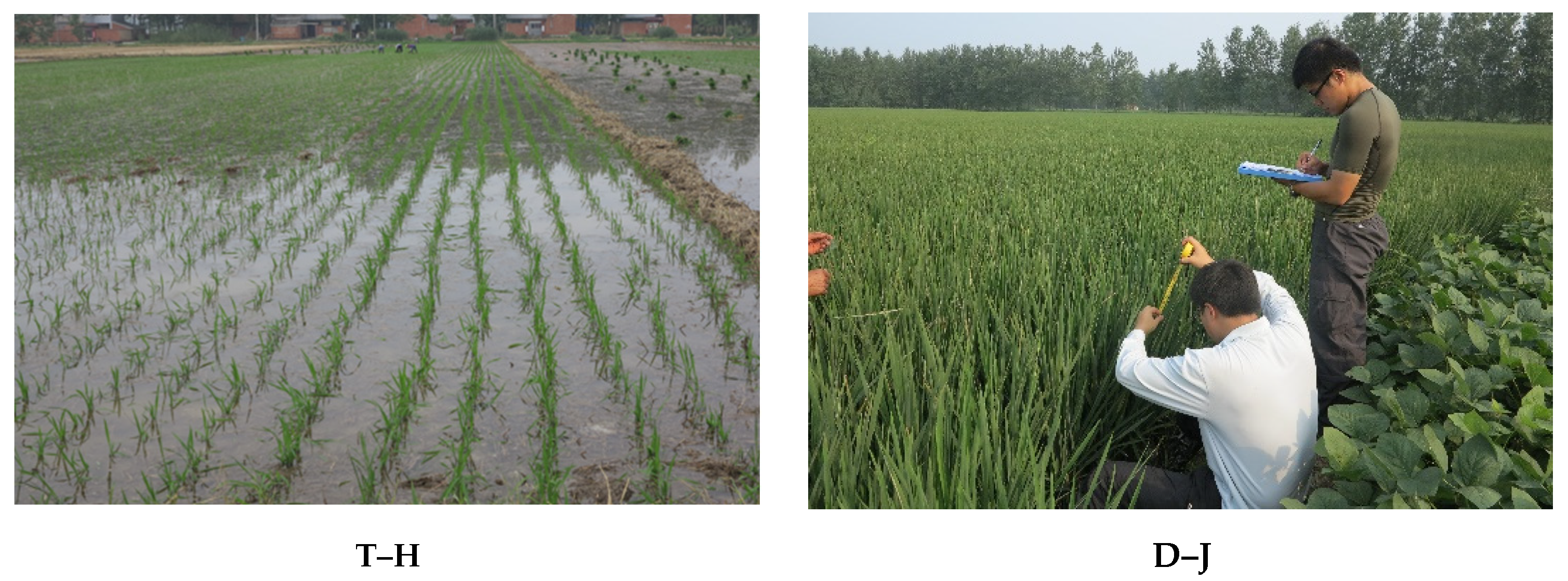
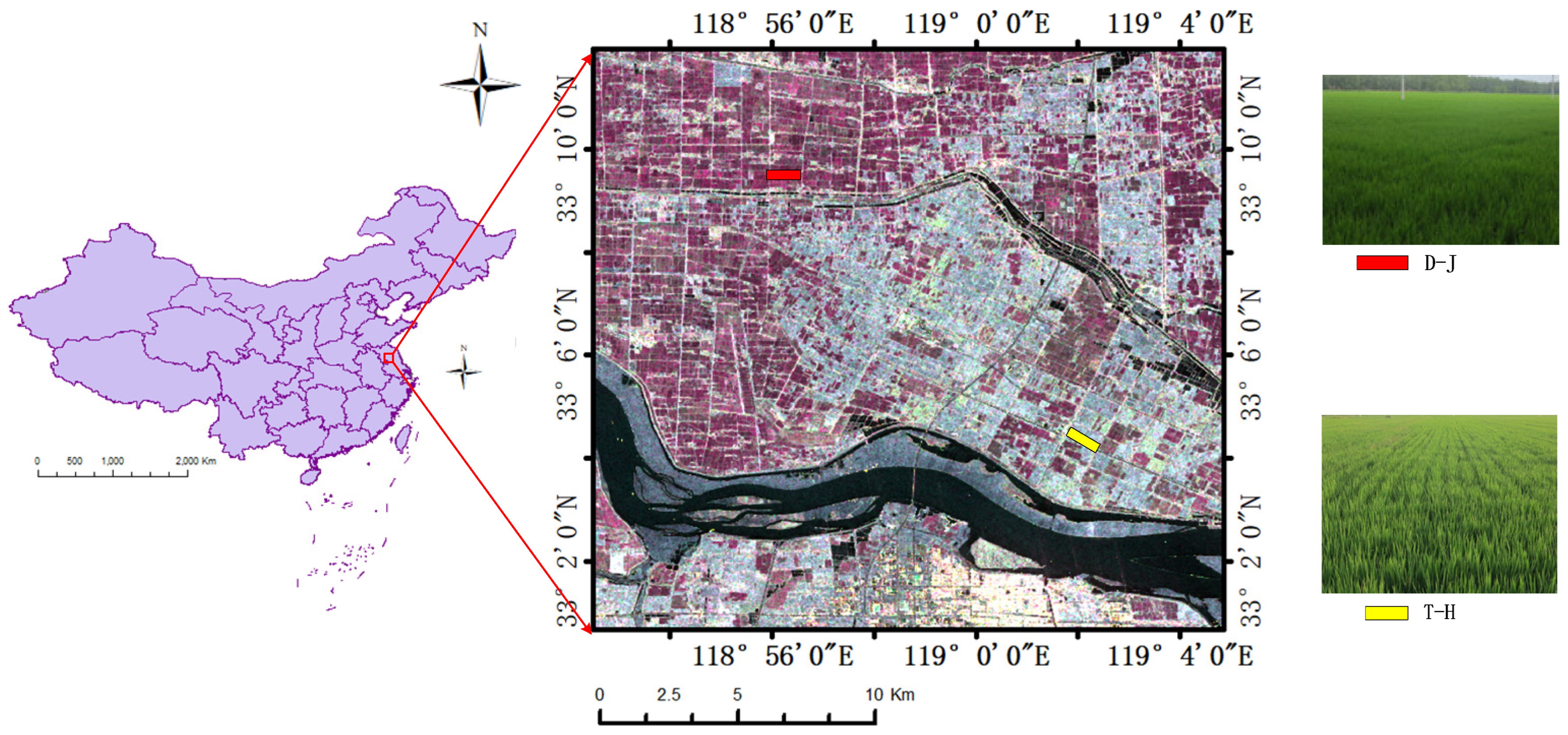
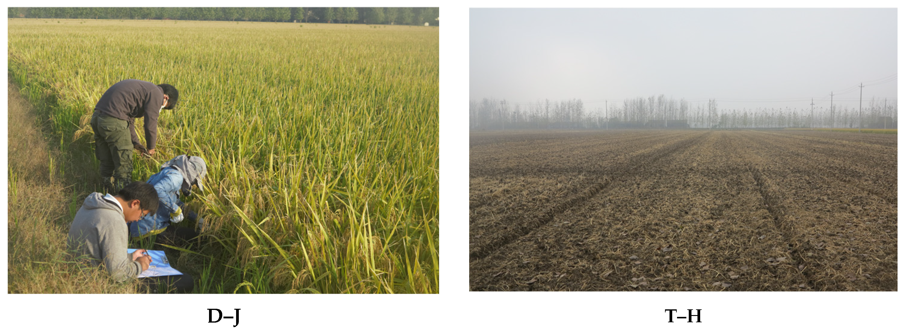
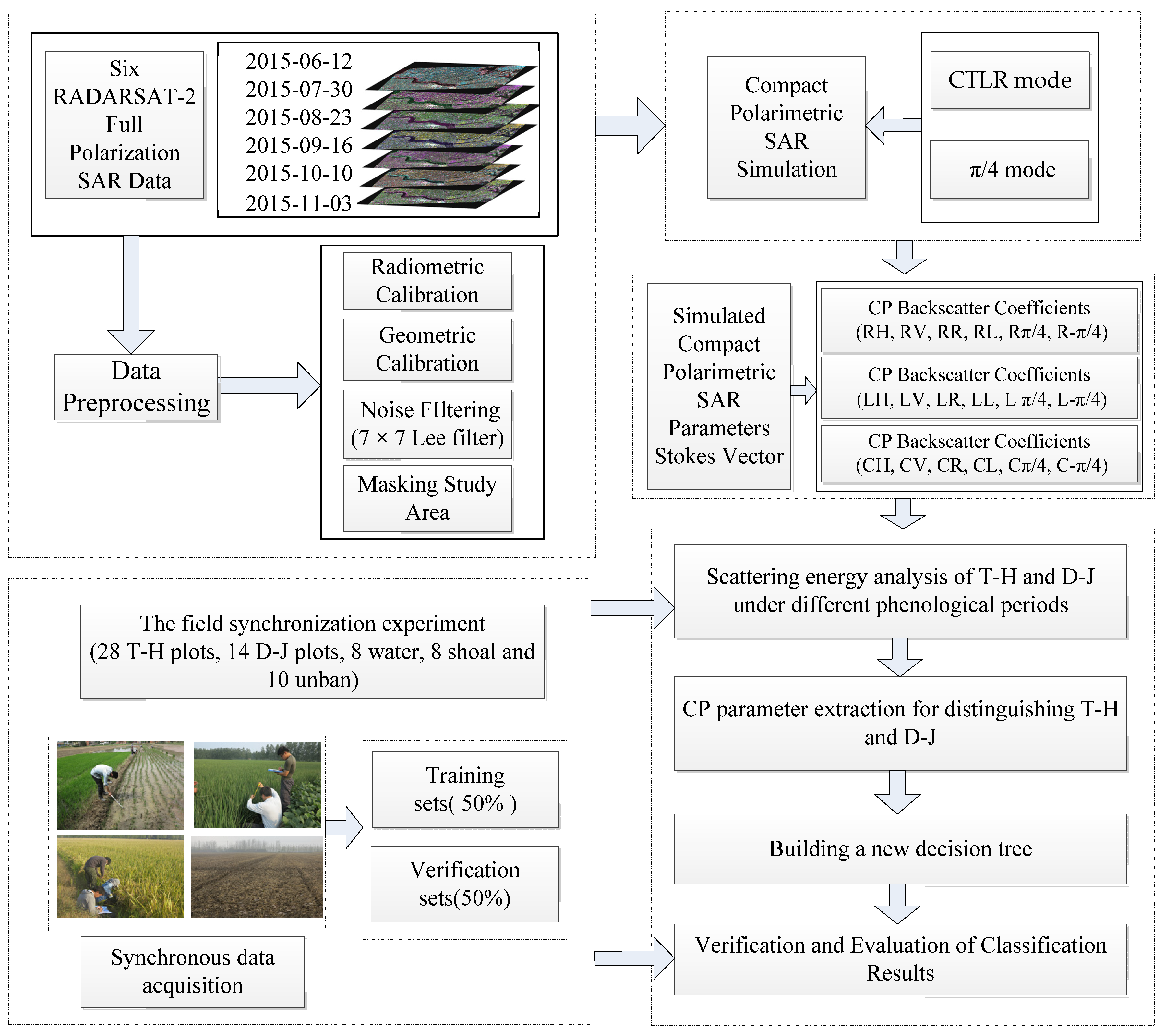
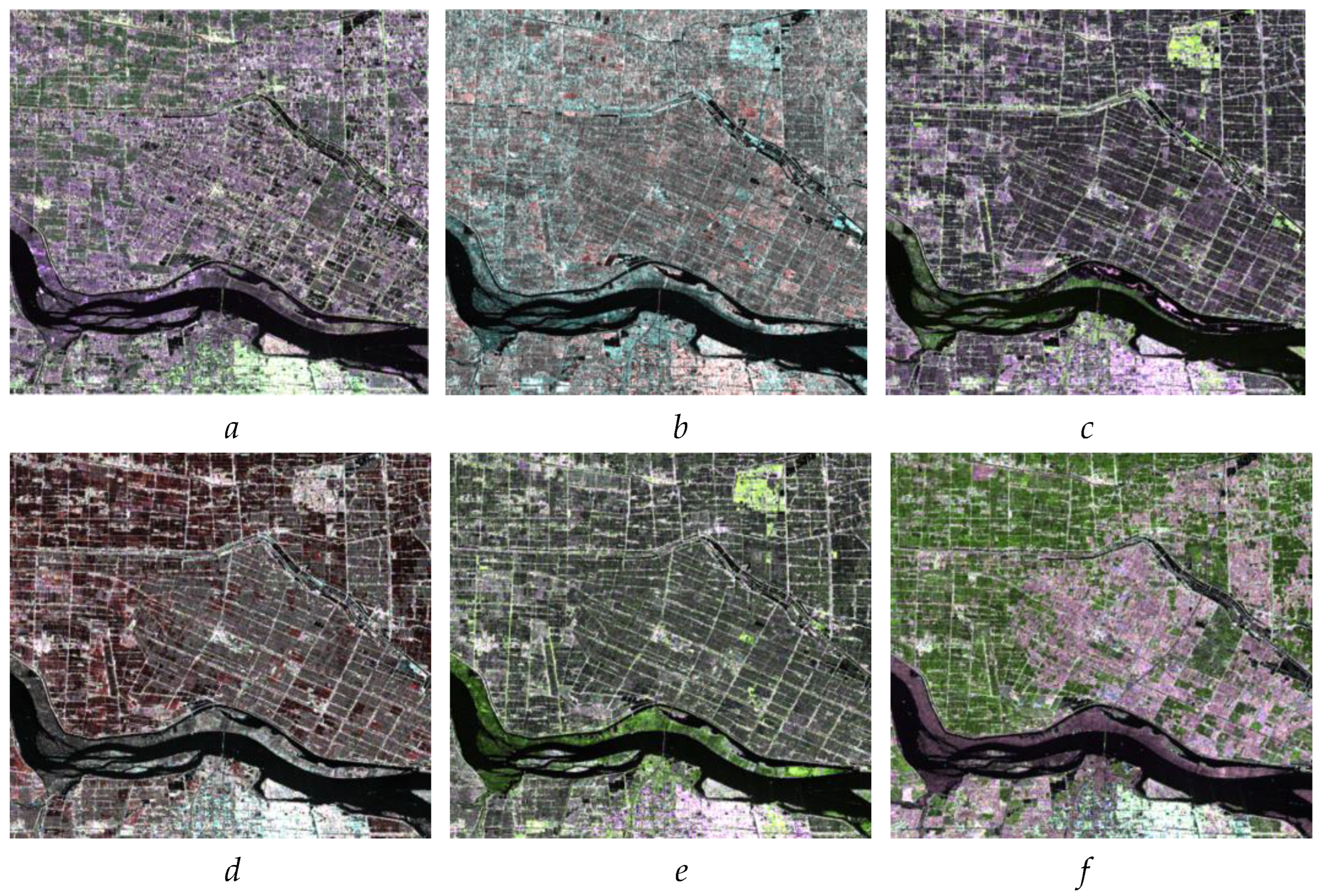
2. Study Area and Data

The study area was located in the lower reaches of the Huaihe River and the west–central part of Jiangsu, which is a major rice-producing area in eastern China. In addition, the scope of the study area was approximately 40 × 30 km, and the central geographic coordinates were 33°07′05″N, 118°59′55.14″E, including areas such as Jinhu, Hongze, and Xuyi of Huai’an, Jiangsu, China (Figure 1). The terrain of the whole study area is high in the west and low in the east, with lake plains in the north, east, and south. The study area is a subtropical temperate monsoon climate zone with a mild climate. The annual mean temperature is 14.6 °C, and the average annual precipitation is 1085 mm.
Rice in this area is cultivated once a year and different farmlands have different choices in rice varieties, planting methods, and growth cycles. The main rice varieties in this study area are hybrid and japonica rice, and the sowing methods are transplanted and direct-sown fields. However, because of the planting techniques and habits of farmers in this area, the main rice classes in the study area are transplanting hybrid rice (T–H) and direct-sown japonica rice (D–J). For T–H, rice seedlings need to be grown in nurseries in advance, and then rice is transplanting by artificial or machine transplanting way of clear row and column. The row and pier spacing should be approximately 30 and 15 cm, respectively. The rice varieties of T–H were LIANGYOU-898 and XIEYOU-9308. For D–J, there was no obvious regularity in the rows and columns for rice seedlings, and the rice varieties were HUAIDAO-5 and NANJING-9108. The D–J plants were shorter than the T–H plants. Moreover, we also demonstrated T–H and D–J by conducting synchronous experiments in the field. Therefore, this experiment was designed to distinguish between T–H and D–J. In the study area, roads and buildings belong to the urban class. In addition, rice is planted in a large area in the study area, and other vegetation consisted of a few trees, which were scattered and did not form a certain area. Therefore, in this paper, combined with the types and distribution areas of ground objects in the study area, we classified the ground objects as T–H, D–J, shoal, water, and urban.
In this paper, a total of six temporal RADARSAT-2 fine-quad, single-look complex (SLC) data were obtained (Table 1). The data center frequency was 5.405 GHZ, and the direction of the satellite track was ascending. The data could evenly cover the rice growth cycle in 2015. Figure 1 shows the color composite images (CP SAR RH (red), RV (green), and RR (blue)) of the backscattering coefficients of simulated CP SAR data on 3 November 2015; in the red box is our study area.
When RADARSAT-2 satellite passed through the study area, we carried out the field synchronization experiment. Firstly, we selected 42 rice sample parcels, including 28 T–H plots and 14 D–J plots in the experimental area. In addition, eight water, eight shoal, and 10 urban plots were also selected. Each sample had an area of more than 120 × 120 m and contained enough pixels. Next, we recorded the position, area, and boundary of the selected plots with a high-precision global positioning system (GPS). The obtained field data included training data and validation data. For the phenology stage of the rice, we recorded according to the Biologische Bundesanstalt, Bundessortenamt und CHemische Industrie (BBCH) [29,30]. The BBCH criteria are the international standard for crop phenology, which uses continuous numbers from 0 to 99 to represent the whole rice growing stage. First, the rice growth stage is divided into three stages: vegetative growth stage (0–39), reproductive stage (40–69), and mature stage (70–99). Then, the three major stages can be further divided into ten smaller phenological stages including budding stage (0–9), seedling stage (10–19), tillering stage (20–29), elongation stage (30–39), booting stage (40–49), heading stage (50–59), flowering stage (60–69), dough stage (70–79), mature stage (80–89), and harvest stage (90–99). Figure 2 shows the field photos taken while we carried out the field synchronization experiment.

3. Methodology

In the study, there were two types of CP mode (three transmitting modes) data. To be specific, the π/4 mode (linear polarization wave in 45° direction, receiving horizontal and vertical polarization echo signals) [5,6] and the CTLR mode [8,9] (transmitting right/left circular polarization, receiving horizontal polarization and vertical polarization) were adopted. The transmitting mode included the left circular, right circular, and linear π/4. In this paper, the CP SAR data of different transmitting and receiving modes were simulated based on six temporal RADARSAT-2 full-polarization SAR data, and the ability of different CP parameters to distinguish two types of rice was explored. Then, we selected the CP parameters that were good for distinguishing the two types of rice paddies, and we built a decision tree model to realize the fine classification of two types of rice paddies. The specific flow chart is shown in Figure 3.
Firstly, we preprocessed 6 temporal RADARSAT-2 full-polarization SAR data, including radiometric calibration, geometric calibration, noise filtering, and masking study area. By comparison, we selected 7 × 7 Lee filter for data noise filtering. Then, based on the pre-processed full-polarization SAR data, Stokes vectors under different transmitting modes were reconstructed, including Stokes vector (SR) of the right circular polarization emission, Stokes vector (SL) of the left circular polarization emission, and Stokes vector Sπ/4 of the π/4 polarization emission. Moreover, the CP backscattering coefficients under three CP transmitting modes were extracted. The scattering intensity of different CP parameters of T–H and D–J rice under different phenology stages were analyzed. Then, we extracted the CP parameters that were good for distinguishing between the two types of rice. A decision tree classification method was established based on the extraction of optimal CP parameters to realize the fine classification of rice. Finally, the classification results were verified by using real ground data (verification sets).

3.1. π/4 Mode and CTLR Mode

The π/4 mode transmits linear polarization waves in a 45° direction, receiving horizontal and vertical polarization echo signals [5,6,31]. The scattering vector k π / 4 is expressed as:
k π / 4 = 1 2 [ S HH + S HV S VV + S HV ] T
C π / 4 = k π / 4 k π / 4 * T = 1 2 [ | S HH | 2 S HH S VV * S VV S HH * | S VV | 2 ] + 1 2 | S HV | 2 [ 1 1 1 1 ] + 1 2 [ 2 Re ( S HH S HV * ) S HH S HV * + S HV S VV * S HH * S HV + S VV S HV * 2 Re ( S VV S HV * ) ]
Furthermore, the last term can be set to 0 based on the assumption of reflectional symmetry. Therefore, the covariance matrix can be simplified to:
C π / 4 = k π / 4 k π / 4 * T = 1 2 [ | S HH | 2 S HH S VV * S VV S HH * | S VV | 2 ] + 1 2 | S HV | 2 [ 1 1 1 1 ]
The CTLR mode is transmitting right/left circular polarization and receiving horizontal polarization and vertical polarization [8,9,31]. The scattering vector k CTLR is expressed as:
k CTLR = 1 2 [ S HH i S HV i S VV + S HV ] T
C CTLR = k CTLR k CTLR * T = 1 2 [ | S HH | 2 i S HH S VV * i S VV S HH * | S VV | 2 ] + 1 2 | S HV | 2 [ 1 i i 1 ] + 1 2 [ 2 Im ( S HH S HV * ) S HH S HV * + S HV S VV * S HH * S HV + S VV S HV * 2 Im ( S VV S HV * ) ]
The same as Cπ/4, the last term can be set to 0 based on the assumption of reflectional symmetry. Therefore, the covariance matrix CCTLR can be simplified to:
C CTLR = k CTLR k CTLR * T = 1 2 [ | S HH | 2 i S HH S VV * i S VV S HH * | S VV | 2 ] + 1 2 | S HV | 2 [ 1 i i 1 ]
Many analyses of compact polarimetry are based on the four-element real Stokes vector of the scattered wave [32,33,34]. Therefore, we generated S vectors under the π/4 and CTLR modes.

3.2. Stokes Vectors under Different CP Modes Are Simulated

Stokes vector reconstruction mainly includes 5 steps. (1) Based on Sinclair matrix of full-polarization SAR data, the electric vector EB of the target backscattering field is constructed when the sensor emits a π/4, left circular, and right circular polarization electromagnetic wave. (2) In the case of a π/4, left circular, right circular, linear polarization (H and V) receiving antenna, and processing system, the corresponding E-π/4, Eπ/4, EL, ER, EH, and EV components are calculated. (3) Four elements of the coherence matrix J(2) are calculated. (4) Stokes vector S is calculated based on the elements of J(2) matrix. (5) The Stokes vector is expressed by using fully polarized data C3 matrix elements instead of J(2) matrix elements.
To describe the process of simulating the S matrix in more detail, we take the transmitting right circular polarization signal as an example, and the Stokes vector calculation formula is as follows (7)–(21).
Step 1: Calculate the electric field vector of the backscattering field EB.
E B = [ Γ ] R ,   R = ( 1 2 ) [ 1 , j ] T = ( 1 2 ) [ S x x j S x y ,   S x y j S y y ] T
where Sxx, Sxy, and Syy are Sinclair matrix elements.
Step 2: Calculate the corresponding EH and EV components.
E H =   [ 1 , 0 ] ,       E B = ( 1 2 ) ( S x x j S x y )
E V =   [ 0 , 1 ] ,   E B = ( 1 2 ) ( S x y j S y y )
Step 3: Calculate four elements of the coherence matrix J(2).
2 J x x = | S x x | 2 + | S x y | 2 + j S x x S x y * j S x y S x x *
2 J x y = S x x S x y * S x y S y y * j | S x y | 2 j S x x S y y *
J y x = J x y *
2 J y y = | S y y | 2 + | S x y | 2 j S y y S x y * + j S x y S y y *
Step 4: Calculate the elements of Stokes vector S.
S 1 = J x x + J y y
S 2 = J x x J y y  
S 3 = Re { S x x S x y * + S x y S y y * } Im S x x S y y *
S 4 = Im { S x x S x y * S x y S y y * } Re S x x S y y * + | S x y | 2
where S1, S2, S3, and S4 are four elements of the Stokes vector.
Step 5: Stokes vectors are expressed using fully polarization data C3 matrix elements.
S 1 = 1 / 2 C 11 + 1 / 2 C 22 + 1 / 2 C 33 + ( 1 / 2 ) Im C 12 + ( 1 / 2 ) Im C 23
S 2 = 1 / 2 C 11 1 / 2 C 33 + ( 1 / 2 ) Im C 12 ( 1 / 2 ) Im C 23
S 3 = ( 1 / 2 ) Re C 12 + ( 1 / 2 ) Re C 23 + Im C 13
S 4 = ( 1 / 2 ) Im C 12 ( 1 / 2 ) Re C 23 + Re C 13 1 / 2 C 22
Through the above five steps, we can also simulate the Stokes vector (SR) of the transmitting right circular polarization wave, the Stokes vector (SL) of the transmitting left circular polarization wave, and the Stokes vector (Sπ/4) of the transmitting π/4 linear polarization wave from the RADARSAT-2 full polarization data.

3.3. The Backscattering Coefficients of Stokes Vector (SR, SL, and Sπ/4) Are Extracted

After Stokes vectors of different transmitting modes are obtained by using Formulas (7)–(21), six backscattering coefficients corresponding to each mode are extracted. Taking the transmitting right circular polarization wave as an example, the calculation formulae of the six backscattering coefficients is shown in Formulas (22)–(27) [35].
σ R H = [ 1 ,   1 ,   0 ,   0 ] × S R
σ R V = [ 1 , 1 ,   0 ,   0 ] × S R
σ R L = [ 1 ,   0 ,   0 ,   1 ] × S R
σ R R = [ 1 ,   0 ,   0 , 1 ] × S R
σ R π 4 = [ 1 ,   0 , 1 ,   0 ] × S R
σ R π 4 = [ 1 ,   0 ,   1 ,   0 ] × S R
Based on the above simulated method, a total of 30 CP parameters under three transmitting modes were obtained for each image, and 10 CP parameters were extracted for each transmitting mode. For the transmitting right circular polarization wave mode, the 10 CP parameters include the backscattering coefficients of RH, RV, RR, RL, R45, and R-45 polarization and the Stokes components (R_S1, R_S2, R_S3, and R_S4). The Stokes matrix represents scattering echo intensity and polarization state, where S1 represents the total power of electromagnetic wave. The backscattering coefficients of RH, RV, RR, RL, R45, and R-45 characterize the echo intensity of the target in RH, RV, RR, RL, R45, and R-45 polarization channels, respectively. For the transmitting left circular polarization wave mode, the 10 CP parameters include the backscattering coefficients of LH, LV, LR, LL, L45, and L-45 polarization and Stokes components (L_S1, L_S2, L_S3, and L_S4). The backscattering coefficients of LH, LV, LR, LL, L45, and L-45 characterize the echo intensity of the target in LH, LV, LR, LL, L45, and L-45 polarization channels, respectively. For the π/4 linear polarization wave mode, the 10 CP parameters include the backscattering coefficients of CH (polarization channel of transmitting linear π/4 and receiving horizontal polarization waves), CV (polarization channel of transmitting linear π/4 and receiving vertical polarization waves), CR (polarization channel of transmitting linear π/4 and receiving right polarization waves), CL (polarization channel of transmitting linear π/4 and receiving left polarization waves), C45 (polarization channel of transmitting linear π/4 and receiving linear π/4 polarization waves) and C-45 (polarization channel of transmitting linear π/4 and receiving linear −π/4 polarization waves) polarization and Stokes components (C_S1, C_S2, C_S3, C_S4). The backscattering coefficients of CH, CV, CR, CL, C45, and C-45 characterize the echo intensity of the target in CH, CV, CR, CL, C45, and C-45 polarization channels, respectively.
For rice, with the growth of rice plant, rice body changes in horizontal and vertical direction, which will lead to changes in surface scattering, volume scattering and double-bounce scattering. For the two types of rice, under the same phenological period, the surface scattering, volume scattering and volume scattering of the two types of rice will be different due to their different planting methods and plant morphology, and then there are differences in the backscattering of different polarization channels. Therefore, the difference of backscattering based on different polarization channels of the two types of rice can be helpful to distinguish the two types of rice.

4. Results and Discussion

In this paper, 30 CP parameters under three transmitting modes in each image were analyzed. We extracted the optional CP parameters that are better for distinguishing the two types of rice (T–H and D–J). Then, a decision tree model was constructed based on the optimal CP parameters to achieve classification.

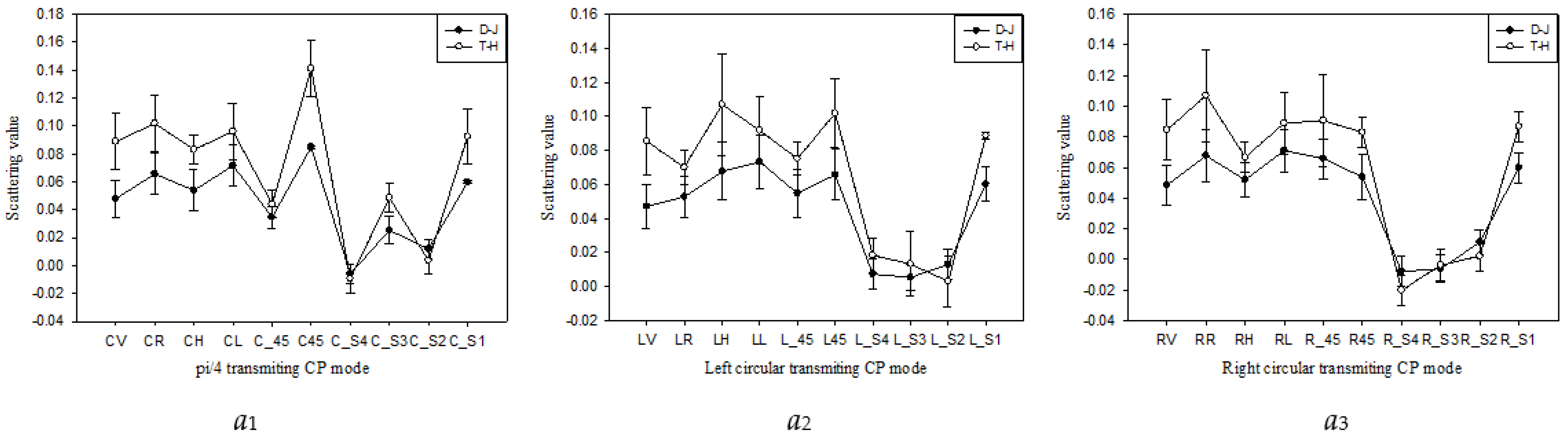
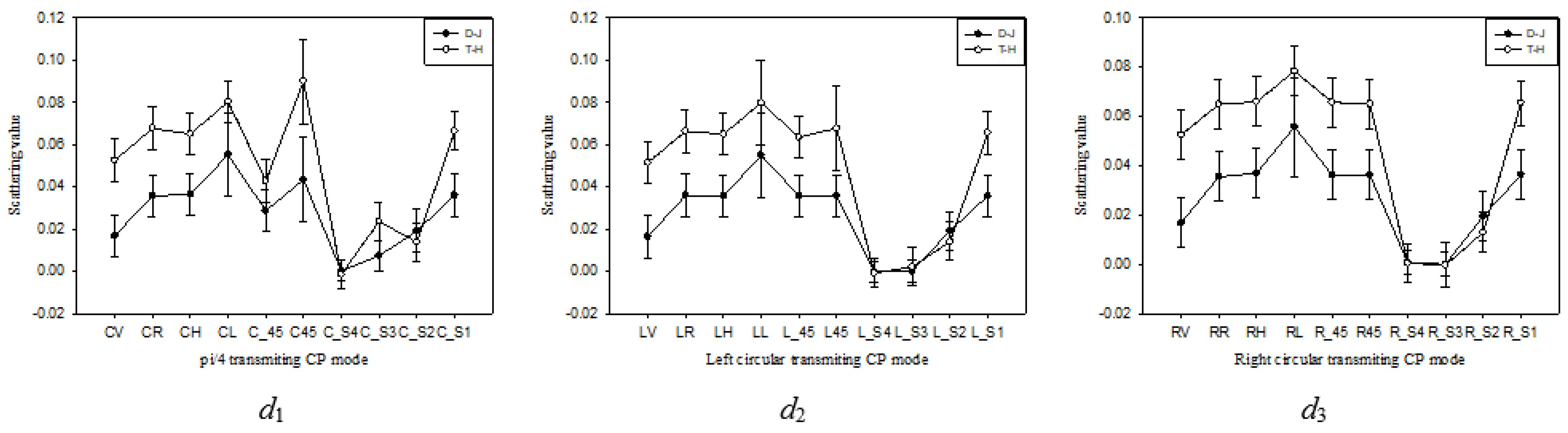
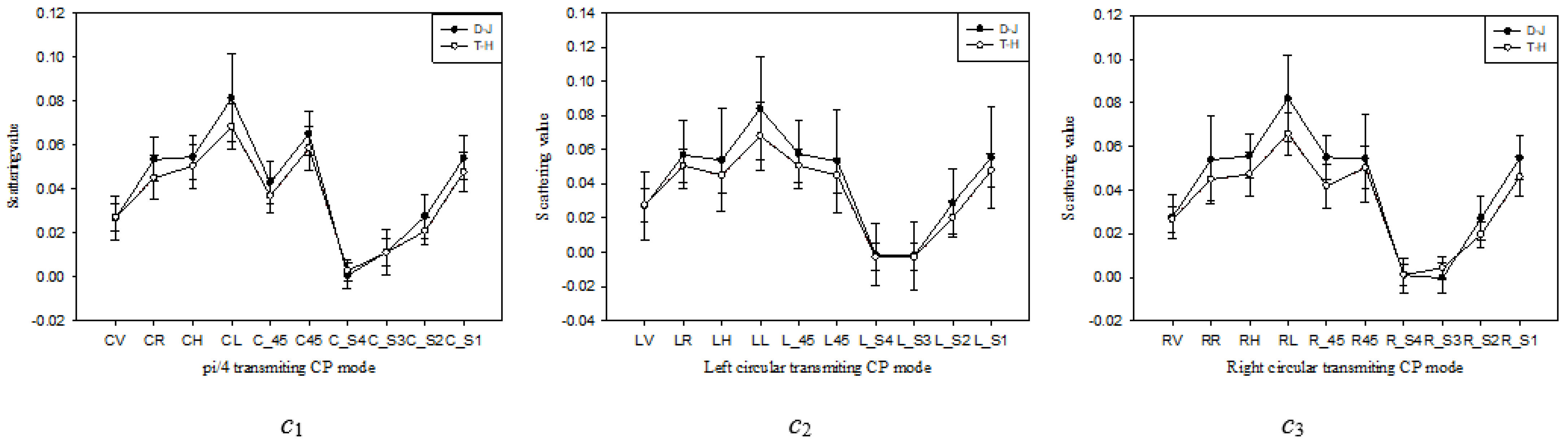
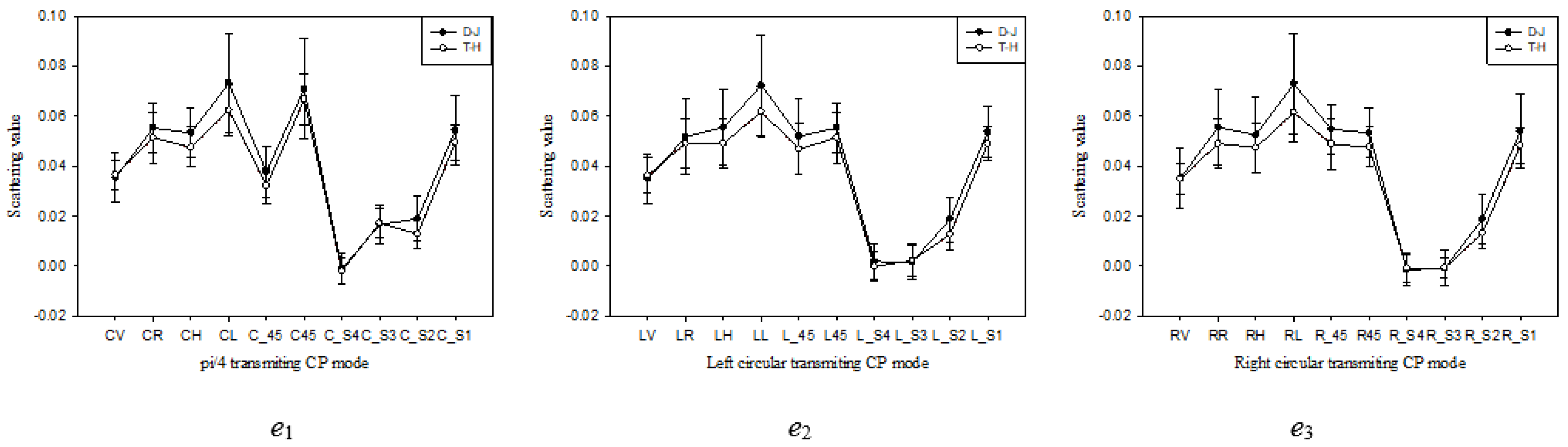
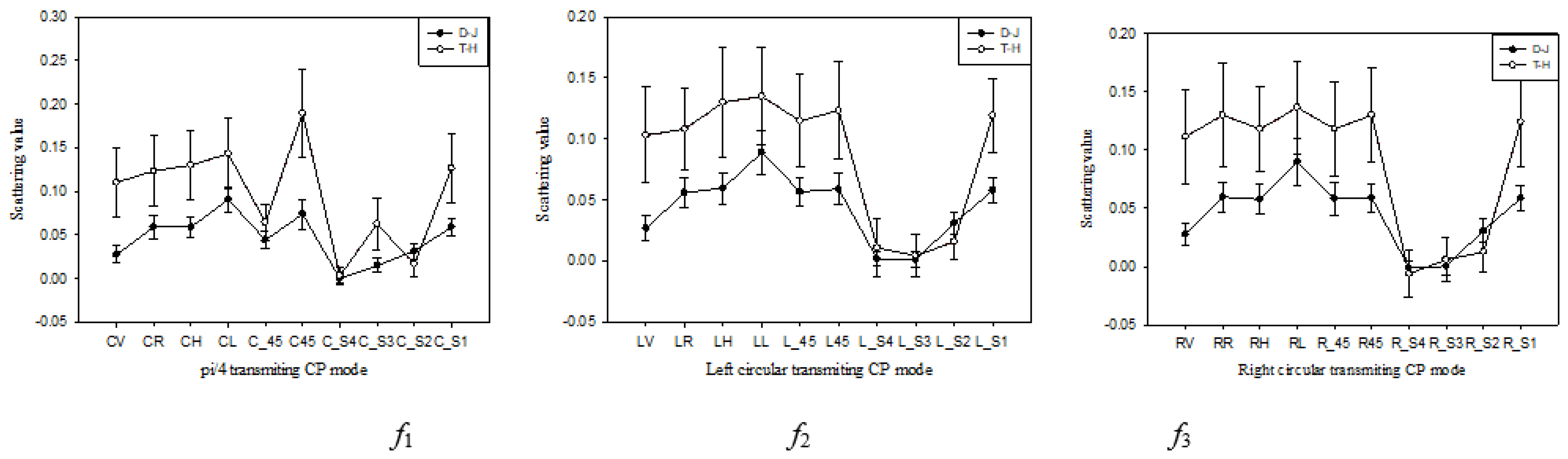
4.1. CP Parameters Analysis of Two Types of Rice under Six Periods

We conducted a statistical analysis on the CP parameters of two types of rice under three transmitting modes in each image and selected the optimal parameters to distinguish the two types of rice. Figure 4, Figure 5, Figure 6, Figure 7, Figure 8 and Figure 9 are the six temporal (i.e., 0612, 0730, 0823, 0916, 1010, and 1103) CP parameters line diagram of two types of rice under three transmitting modes.
As can be seen from CP parameters (transmitting linear π/4, left circular, and right circular polarization modes) in 0612 period (Figure 4), the scattering value of T–H under each transmitting mode was greater than D–J. The main reason was that the rice phenology stage in the D–J paddy was the seedling stage around June 12, while in the T–H paddy, the rice had not been planted and was basically a bare land type. Therefore, the T–H scattering value was larger than D–J for each polarization channel. As can be seen from the line diagram in Figure 4a1a3, the C45 parameter in a1 shows the most obvious difference between the two types of rice, the LV parameter in a2 shows the most obvious difference between the two types of rice, and the RR parameter in a3 shows the most obvious difference between the two types of rice.
As can be seen from Figure 5, the scattering value of D–J under each transmitting mode was greater than T–H. At this period, the T–H was in the seedling stage, and the underlying surface of the paddy was water, which resulted in the T–H’s underlying surface being more likely to form a mirror reflection. However, the planting method of D–J is sowing, and the underlying surface was bare soil. It is not easy to form a mirror reflection. Therefore, the scattering of each channel in the T–H paddy was generally lower than that of D–J in this period. As can be seen from the line diagram of Figure 5b1b3, the CL, LL, and RR parameters in b1, b2, and b3 show the most obvious difference between the two types of rice.
The phenology stage of T–H and D–J was the booting–heading stage on 23 August 2015. As can be seen from Figure 6, the scattering value of D–J under each transmitting mode was greater than T–H. However, the CP parameters’ difference between the two types rice in the 0730 period became smaller. The reason was that with the growth of T–H, the underlying surface was gradually covered by rice plants, and the underlying surface was no longer prone to specular scattering. The phenology stage of T–H and D–J was the booting–heading stage. As can be seen from the line diagram in Figure 6c1c3, the CL parameter in c1 shows the most obvious difference between the two types of rice, the LL parameter in c2 shows the most obvious difference between the two types of rice, and the RL parameter in c3 shows the most obvious difference between the two types of rice.
As can be seen from Figure 7, scattering value of T–H under each transmitting mode was greater than D–J. The main reason was that planting method of T–H is transplanting seedlings, and with the growth of rice plants, the plants easily form double-bounce scattering with the underlying surface. However, the planting method of D–J is sowing, which makes it difficult to form double-bounce scattering with the underlying surface. In addition, the phenology stage of T–H and D–J was the heading–flowering stage on September 16, 2015. The difference in the rice ears between T–H and D–J also resulted in the difference in the scattering intensity to some extent. As can be seen from the line diagram in Figure 7d1d3, the C45 parameter in d1 shows the most obvious difference between the two types of rice, the LV parameter in d2 shows the most obvious difference between the two types of rice, and the RV parameter in d3 shows the most obvious difference between the two types of rice. In the three transmitting modes, the receiving signals of left circular mode showed the most significant difference between the two types of rice.
The phenology stage of T–H and D–J was the dough–mature stage on 10 October 2015. As can be seen from Figure 8, there was no significant difference between the scattering value of T–H and D–J in the polarization channels under each transmitting mode. The main reason was that with the growth of the rice plants, the rice in this period was in the mature stage, and the underlying surface was basically completely covered. The scattering of the two types of rice was mainly body scattering and surface scattering, and there was little difference in the total scattering between the two types of rice. Therefore, it was very difficult to distinguish the two types of rice in each channel. As can be seen from the line diagram in Figure 8e1e3, comparatively speaking, the CL parameter in e1 shows the most obvious difference between the two types of rice, the LL parameter in e2 shows the most obvious difference between the two types of rice, and the RL parameter in e3 shows the most obvious difference between the two types of rice. Similar to the 0823 period, the scattering values of the two types of rice were significantly different when receiving the left circular polarization wave.
As can be seen from Figure 9, there was a significant difference between the scattering values of T–H and D–J in the polarization channels under each transmitting mode. Because T–H was in the harvest period, the paddy was bare after harvest, while the plants in the D–J paddy had not been harvested. Compared with the scattering intensity of the two types of rice, T–H was obviously larger than D–J. As can be seen from the line diagram of Figure 9f1f3, the C45 parameter in f1 shows the most obvious difference between the two types of rice, the LH\LV parameter in f2 shows the most obvious difference between the two types of rice, and the RV parameter in f3 shows the most obvious difference between the two types of rice.
The six temporal CP parameters of the three transmitting modes were statistically analyzed, and the optimal CP parameters for distinguishing T–H and D–J in each transmitting mode were obtained as shown in Table 2. As shown in the Figure 10, an optimal CP parameter from each of the three modes was used as a channel for color composite images under each period based on Table 2.
It can be seen from Figure 10a–g that the scattering intensities of the two types of rice were very different. Among them, the difference between T–H and D–J in Figure 10g was the most obvious. Since T–H as in the harvest period on 3 November, the plants were harvested, as shown in the red box in the Figure 10g. However, D–J had a later harvest period than T–H and had not been harvested, as shown in the yellow box in the Figure 10g.
In order to more clearly characterize the degree of difference between T–H and D–J in the optimal CP parameters, based on Table 2, we made a histogram of the difference (|CPT–H-CPD–J|) in scattering intensities of the two types of rice under the three modes under six periods (Figure 10).
As can be seen from Figure 11, among the six periods of rice growth, the difference between the two types of rice was most obvious in the 1103 period, and the three CP parameters in the 1103 period (1103-C45, 1103_LV, and 1103_RV) were most obvious in distinguishing the two rice species, especially 1103_C45. Moreover, in addition to the optimal CP parameters in the 1103 period, the characterizations of distinguishing T–H and D–J in the 0730, 0612, and 0916 periods were also obvious, especially 0612_C45, 0730_LL,0730_CL,0730_RR, and 0916_C45. However, there was no obvious differences between the two rice varieties in the 0823 and 1010 period.

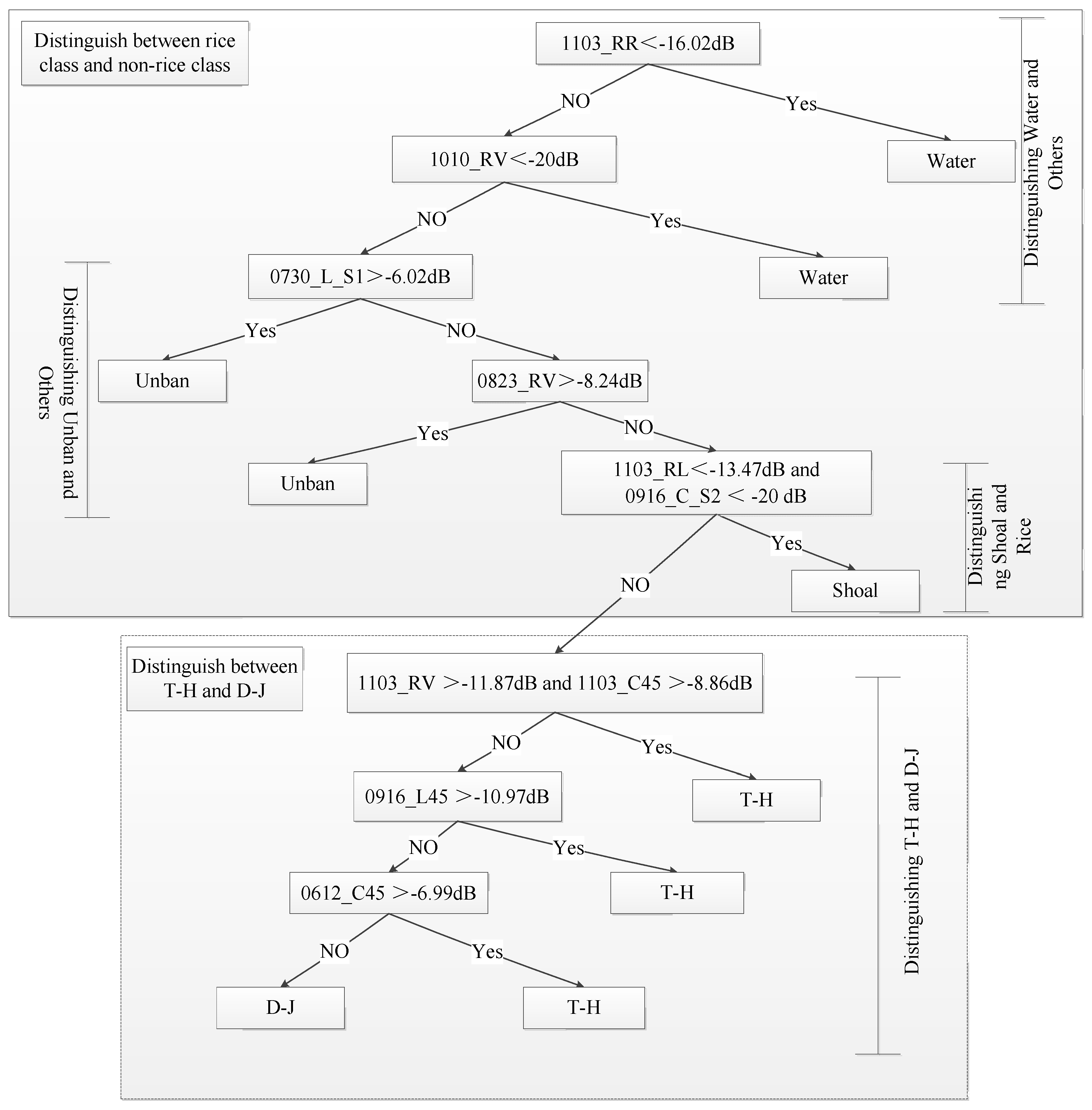
4.2. Building a Decision Tree Classification Model

As shown in Figure 12, we built a decision tree classification model based on optimizing CP parameters under three transmitting modes. First, rice class and non-rice classes are distinguished. For non-rice classes, it was easy to distinguish them from each other due to the obvious differences in scattering intensity between water, urban, and shoal. Therefore, in the first step, we used backscattering coefficients (1103_RR and 1010_RV) to distinguish water from other ground objects. The two temporal (1010 and 1103 periods) backscattering coefficients were selected to exclude the influence of moving targets on the river surface. In the second step, we distinguished urban and other classes. Since the scattering intensity of 0730_L_S1 and 0823_RV of cities was obviously higher than that of other ground objects, we used these two parameters to classify cities and other classes. In the third step, we distinguished shoal and rice classes. Through statistical analysis, we found that 1103_RL and 0916_C_S2 were significantly different between shoal and rice classes. Therefore, these two parameters were used to distinguish shoal from rice classes.
In addition, the most important thing in this paper was to distinguish T–H and D–J. It can be seen from Figure 11 that the scattering intensity difference of the three optimal parameters in the 1103 period was the most obvious. This was because T–H was in the harvest stage (1103 period). Therefore, we first used two parameters, 1103_RV and 1103_C45, to distinguish the harvested T–H class and other rice. Then, the other unharvested T–H and D–J were distinguished by the optimal parameters (0916_L45 and 0612_C45) of other periods. The reason we used 0916_L45 was that the planting method of T–H is transplanting seedlings, and with the growth of rice plants, the plants easily form double-bounce scattering with the underlying surface in the 0916 period. Therefore, the scattering value of T–H under each transmitting mode was greater than D–J (Figure 7) and, in particular, 0916_L45 (Figure 11) was the most obvious for distinguishing T–H and D–J. In addition, the reason we selected 0612_C45 was that the rice phenology stage in the D–J paddy was in the seedling stage around June 12, while in the T–H paddy, rice had not been planted and the paddy was basically a bare land type. Therefore, the T–H scattering value was larger than D–J under each transmitting mode (Figure 4) and, in particular, 0612_C45 (Figure 11) was the most obvious for distinguishing T–H and D–J.

4.3. Classification and Accuracy Verification

We used the constructed decision tree model (Figure 12) for decision tree classification based on the optimal CP parameters of the three transmitting modes. Among them, 50% of the sample data were used as training data, and the remaining 50% sample data were used as verification data. Training and verification data were randomly selected without overlap. The final classification result based on the decision tree classification method is shown in Figure 13.
As can be seen from Figure 13, urban, water, and shoal were clearly distinguished, which is related to the large difference in scattering characteristics between these three classes and two types of rice classes. Water were mainly concentrated in river areas, and shoal class is mainly distributed on both sides of the Huaihe River. Moreover, urban was mainly concentrated in Jinhu in the south of the study area, and villages and roads were distributed in the study area. In addition to non-rice classes, rice classes were divided into two types. T–H was mainly distributed in the southeast region and the south bank of the river, while D–J was mainly distributed in the northwest, which is consistent with the actual distribution of rice in the study area.
Furthermore, we could obtain the confusion matrix (Table 3) based on the final classification result and real ground sampling data. As can be seen from Table 3, the overall classification accuracy was 96.16%, and the kappa coefficient was 0.948. The user accuracy of the water, urban, shoal, T–H, and D–J classes were 99.84%, 100.00%, 96.01%, 90.82%, and 92.18%, respectively. In general, the user accuracy of the five classes was above 90%, and the mapping accuracy was above 81%. The average accuracy of T–H and D–J was above 94% and 86%, respectively. Therefore, the classification accuracy was satisfactory.
From commission and omission error, it was found that the main classification error of the T–H and D–J came from the confusion between the two types of rice, which was mainly due to the fact of their similar radar responses. Compared with T–H, the classification accuracy of D–J was lower, especially the mapping accuracy, which may be due to the relatively less training and verification sample data.

5. Conclusions

In this paper, CP SAR data of three transmitting modes (transmitting linear π/4, left circular polarization, and right circular polarization) were simulated based on multi-temporal full polarimetric RADARSAT-2 C band data. By statistical analysis of the scattering intensities of CP parameters of six temporal CP SAR data under three transmitting modes, the optimal parameters for distinguishing two types of rice were obtained. Finally, a decision tree classification model was established based on optimal parameters to carry out rice classification. The classification results can provide more accurate information for rice growth monitoring and yield estimation in the study area. The specific conclusions are as follows:
(1)
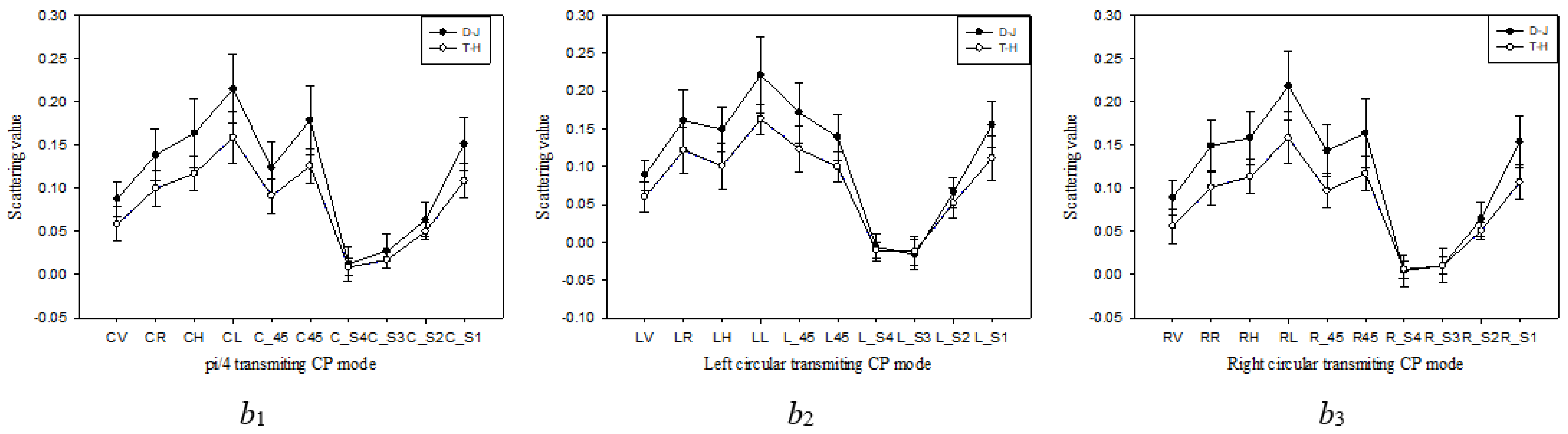
Through statistical analysis of the scattering intensities of CP parameters of six temporal CP SAR data under three transmitting modes, we found that CP parameters in the 1103 period (harvest stage) were the best parameters to distinguish between the two types of rice, followed by 0730 (seedling–elongation stage), 0612 (seedling stage), and 0916 (heading–flowering stage) periods. Moreover, CP SAR parameters in 0823 (booting–heading stage) and 1010 (dough–mature stage) periods were not obvious to be able to distinguish between T–H and D–J;
(2)
Firstly, in the CP SAR parameters of the three modes during the 1103 period, 1103_C45, 1103_LV, and 1103_RV were the most obvious to distinguish T–H and D–J. Secondly, in the CP SAR parameters under three transmitting modes during the 0730 period, 0730_CL, 0730_LL, and 0730_RL were also obvious to distinguish T–H and D–J. As can be seen from the optimal parameters of the 0730 period, all three CP parameters were for the best for the case of left circular polarization reception. In addition, in the 0612 period, 0612_C45, 00612_LV, and 0730_RR clearly distinguished between T–H and D–J; in the 0916 period, 0916_C45, 0916_LV, and 0916_RV were consistent with the optimal parameter polarization channels in the 1103 period;
(3)
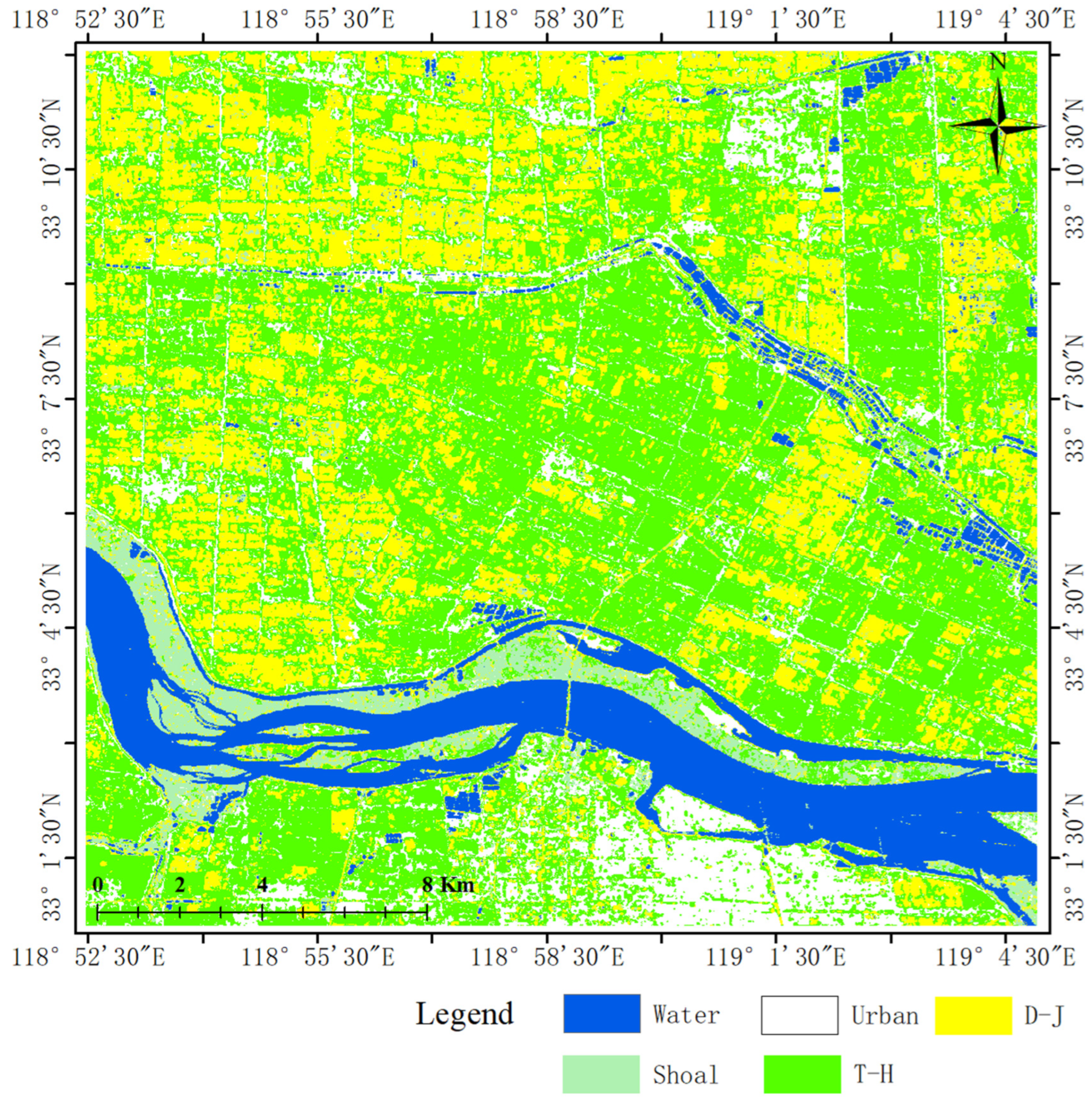
Based on the optimal CP parameters, we established a new decision tree classification model for rice classification, with an overall classification accuracy of more than 95% and a kappa coefficient of more than 0.94. It can be seen that high-precision rice classification results were obtained. Compared with T–H, the classification accuracy of D–J was lower, which may be due to the relatively fewer training and verification sample data. Another reason for the lower classification accuracy of D–J than T–H was that the two rice varieties and planting methods and environments were different. The T–H planting method is transplanting, and its plots were regular and square compared with D–J, while the D–J planting method is the direct-sown planting method and has an irregular distribution. Thus, in both types of rice samples, T–H was more accurate than D–J, and this is an important reason for why T–H obtained a higher accuracy than D–J.
There are two main aspects to the future work of this research, specifically:
(1)
We will consider exploring the ability of CP parameters to distinguish other crops (leeks, wheat, sugar beet, etc.) under different transmitting and receiving modes for the fine classification of other crops;
(2)
We will consider applying the results of rice fine classification based on multiple mode CP parameters to yield estimation.

Author Contributions

Data curation, Y.S.; Formal analysis, X.G.; Funding acquisition, J.Y. (Junjun Yin), and K.L.; Methodology, J.Y. (Junjun Yin) and X.G.; Project administration, J.Y. (Jian Yang); Resources, Y.S.; Supervision, J.Y. (Junjun Yin); Validation, K.L.; Writing—original draft, X.G.; Writing—review & editing, X.G. and J.Y. (Junjun Yin). All authors have read and agreed to the published version of the manuscript.

Funding

This work was funded in part by NSFC under grants 62171023 and 41871272, the Fundamental Research Funds for the Central Universities under grant FRF-GF-20-17B, the Scientific and Technological Innovation Foundation of Shunde Graduate School, USTB, under grant BK20BF012.

Institutional Review Board Statement

Not applicable.

Informed Consent Statement

Informed consent was obtained from all subjects involved in the study.

Data Availability Statement

Not applicable.

Acknowledgments

The authors would like to acknowledge the guidance and help in compact polarimetric SAR of Brian Brisco from the Canada Centre for Mapping and Earth Observation, Natural Resources Canada.

Conflicts of Interest

The authors declare no conflict of interest.

References

  1. Maclean, J.L.; Dawe, D.C.; Hardy, B.; Hettel, G.P. Rice Almanac: Source Book for the Most Important Economic Activity on Earth; International Rice Research Institute (IRRI): Los Banos, Philippines, 2002. [Google Scholar]
  2. Guo, H.; Li, X. Technical Characteristics and Potential Application of the New Generation SAR for Earth Observation. Chin. Sci. Bull. 2011, 56, 1155–1168. [Google Scholar]
  3. Zhang, H.; Xie, L.; Wang, C.; Zhang, B.; Wu, F.; Tang, Y.X. Information Extraction Application of Compact Polarimetric SAR Data. J. Image Graph. 2013, 18, 1065–1073. [Google Scholar]
  4. Yang, H. Study on Quantitative Crop Monitoring by Time Series of Fully Polarimetric and Compact Polarimetric SAR Imagery; Chinese Academy of Forestry: Beijing, China, 2015. [Google Scholar]
  5. Souyris, J.C.; Imbo, P.; Fjortoft, R.; Sandra, M.; Lee, J.S. Compact Polarimetry Based on Symmetry Properties of Geophysical Media: The π/4 Mode. IEEE Trans. Geosci. Remote Sens. 2005, 43, 634–646. [Google Scholar] [CrossRef]
  6. Souyris, J.C.; Mingot, S. Polarimetry Based on One Transmitting and Two Receiving Polarizations: The π/4 Mode. In Proceedings of the 2002 IEEE International Geoscience and Remote Sensing Symposium (IGARSS), Toronto, ON, Canada, 24–28 June 2002. [Google Scholar]
  7. Stacy, N.; Preiss, M. Compact Polarimetric Analysis of X-Band SAR Data. In Proceedings of the EUSAR 2006-6th European Conference on Synthetic Aperture Radar, Dresden, Germany, 16–18 May 2006. [Google Scholar]
  8. Raney, R.K. Dual-Polarized SAR and Stokes Parameters. IEEE Geosci. Remote Sens. Lett. 2006, 3, 317–319. [Google Scholar] [CrossRef]
  9. Raney, R.K. Hybrid-Polarity SAR Architecture. IEEE Trans. Geosci. Remote Sens. 2007, 45, 3397–3404. [Google Scholar] [CrossRef] [Green Version]
  10. Yin, J.; Papathanassiou, K.; Yang, J. Formalism of Compact Polarimetric Descriptors and Extension of the ∆αB/αB Method for General Compact-Pol SAR. IEEE Trans. Geosci. Remote Sens. 2019, 57, 10322–10335. [Google Scholar] [CrossRef]
  11. Panigrahi, R.K.; Mishra, A.K. Comparison of Hybrid-Pol with Quad-Pol Scheme Based on Polarimetric Information Content. Int. J. Remote Sens. 2012, 33, 3531–3541. [Google Scholar] [CrossRef]
  12. Nord, M.; Ainsworth, T.; Lee, J. Comparison of Compact Polarimetric Synthetic Aperture Radar Modes. IEEE Trans. Geosci. Remote Sens. 2009, 47, 174–188. [Google Scholar] [CrossRef]
  13. Collins, M.; Denbina, M.; Atteia, G. On the Reconstruction of Quad-Pol SAR Data from Compact Polarimetry Data for Ocean Target Detection. IEEE Trans. Geosci. Remote Sens. 2013, 51, 591–600. [Google Scholar] [CrossRef]
  14. Yin, J.; Papathanassiou, K.; Yang, J.; Chen, P. Least-Squares Estimation for Pseudo Quad-Pol Image Reconstruction from Linear Compact Polarimetric SAR. IEEE J. Sel. Top. Appl. Earth Obs. Remote Sens. 2019, 12, 3746–3758. [Google Scholar] [CrossRef]
  15. Yin, J.; Yang, J. Framework for Reconstruction of Pseudo Quad Polarimetric Imagery from General Compact Polarimetry. Remote Sens. 2021, 13, 530. [Google Scholar] [CrossRef]
  16. Xie, Q.; Wang, J.; Liao, C.; Shang, J.; Lopez-Sanchez, J.M.; Fu, H.; Liu, X. On the Use of Neumann Decomposition for Crop Classification Using Multi-Temporal RADARSAT-2 Polarimetric SAR Data. Remote Sens. 2019, 11, 776. [Google Scholar] [CrossRef] [Green Version]
  17. Ohki, M.; Shimada, M. Large-Area Land Use and Land Cover Classification With Quad, Compact, and Dual Polarization SAR Data by PALSAR-2. IEEE Trans. Geosci. Remote Sens. 2018, 56, 5550–5557. [Google Scholar] [CrossRef]
  18. Mandal, D.; Ratha, D.; Bhattacharya, A.; Kumar, V.; McNairn, H.; Rao, Y.; Frery, A. A Radar Vegetation Index for Crop Monitoring Using Compact Polarimetric SAR Data. IEEE Trans. Geosci. Remote Sens. 2020, 58, 6321–6335. [Google Scholar] [CrossRef]
  19. Guo, X.; Li, K.; Shao, Y.; Wang, Z.; Li, H.; Yang, Z.; Liu, L.; Wang, S. Inversion of Rice Biophysical Parameters Using Simulated Compact Polarimetric SAR C-Band Data. Sensors 2018, 18, 2271. [Google Scholar] [CrossRef] [PubMed] [Green Version]
  20. Gao, G.; Gao, S.; He, J.; Li, G. Adaptive Ship Detection in Hybrid-Polarimetric SAR Images Based on the Power-Entropy Decomposition. IEEE Trans. Geosci. Remote Sens. 2018, 55, 5394–5407. [Google Scholar] [CrossRef]
  21. Gao, G.; Gao, S.; He, J.; Li, G. Ship Detection Using Compact Polarimetric SAR Based on the Notch Filter. IEEE Trans. Geosci. Remote Sens. 2018, 56, 5380–5393. [Google Scholar] [CrossRef]
  22. Zhang, T.; Wang, W.; Yang, Z.; Yin, J.; Yang, J. Ship Detection From PolSAR Imagery Using the Hybrid Polarimetric Covariance Matrix. IEEE Geosci. Remote Sens. Lett. 2021, 18, 1575–1579. [Google Scholar] [CrossRef]
  23. Ghanbari, M.; Clausi, D.; Xu, L.; Jiang, M. Contextual Classification of Sea-Ice Types Using Compact Polarimetric SAR Data. IEEE Trans. Geosci. Remote Sens. 2019, 57, 7476–7491. [Google Scholar] [CrossRef]
  24. Wang, X.; Shao, Y.; Zhang, F.; Tian, W. Comparison of C- and L-band Simulated Compact Polarized SAR in Oil Spill Detection. Front. Earth Sci. 2019, 13, 351–360. [Google Scholar] [CrossRef]
  25. Guo, X.; Li, K.; Wang, Z.; Li, H.; Yang, Z. Fine Classification of Rice with Multi-Temporal Compact Polarimetric SAR Based on SVM+SFS Strategy. Remote Sens. Land Resour. 2018, 30, 20–27. [Google Scholar]
  26. Uppala, D.; Somepalli, V.; Venkata, R.K.; Rama, S. Identification of Optimal Single Date for Rice Crop Discrimination and Relationships Between Backscatter and Biophysical Parameters Using RISAT-1 Hybrid Polarimetric SAR Data. Geocarto Int. 2019, 36, 2010–2022. [Google Scholar] [CrossRef]
  27. Uppala, D.; Kothapalli, R.V.; Poloju, S.; Mullapudi, S.; Dadhwal, V. Rice Crop Discrimination Using Single Date RISAT1 Hybrid (RH, RV) Polarimetric Data. Photogramm. Eng. Remote Rens. 2015, 81, 557–563. [Google Scholar] [CrossRef]
  28. Yang, Z.; Li, K.; Liu, L.; Shao, Y.; Brisco, B.; Li, W. Rice Growth Monitoring Using Simulated Compact Polarimetric C band SAR. Radio Sci. 2014, 49, 1300–1315. [Google Scholar] [CrossRef]
  29. Zadoks, J.C.; Chang, T.T.; Konzak, C.F. A decimal code for the growth stages of cereals. Weed Res. 1974, 14, 415–421. [Google Scholar] [CrossRef]
  30. Hess, M.; Barralis, G.; Bleiholder, H.; Buhr, L.; Eggers, T.H.; Hack, H.; Stauss, R. Use of the extended BBCH scale—General for the descriptions of the growth stages of mono and dicotyledonous weed species. Weed Res. 1997, 37, 433–441. [Google Scholar] [CrossRef]
  31. Wang, X.; Shao, Y.; She, L.; Tian, W.; Li, K.; Liu, L. Ocean Wave Information Retrieval Using Simulated Compact Polarized SAR from Radarsat-2. J. Sens. 2018, 2018, 1738014. [Google Scholar] [CrossRef] [Green Version]
  32. Li, H.; Perrie, W.; He, Y.; Lehner, S.; Brusch, S. Target detection on the ocean with the relative phase of compact polarimetry SAR. IEEE Trans Geosci. Remote Sens. 2013, 51, 3299–3305. [Google Scholar] [CrossRef]
  33. Charbonneau, F.; Brisco, B.; Raney, R.; McNairn, H.; Liu, C.; Vachon, P.W.; Shang, J.; DeAbreu, R.; Champagne, C.; Merzouki, A.; et al. Compact polarimetry overview and applications assessment. Can. J. Remote Sens. 2010, 36, 298–315. [Google Scholar] [CrossRef]
  34. Guo, S.; Li, Y.; Hong, W.; Wang, J.; Guo, X. Model-based target decomposition with the π/4 mode compact polarimetry data. Sci. China Inf. Sci. 2016, 59, 062307. [Google Scholar] [CrossRef]
  35. Dabboor, M.; Geldsetzer, T. Towards sea ice classification using simulated RADARSAT Constellation Mission compact polarimetric SAR imagery. Remote Sens. Environ. 2014, 140, 189–195. [Google Scholar] [CrossRef]
Figure 1. The color composite images (CP SAR RH (red), RV (green), and RR (blue)) of the backscattering coefficients of simulated CP SAR data on 3 November 2015; in the red box is our study area.
Remotesensing 14 01644 g001
Figure 2. The field synchronization experiment photos.
Remotesensing 14 01644 g002aRemotesensing 14 01644 g002b
Figure 3. The specific flow chart.
Remotesensing 14 01644 g003
Figure 4. The CP parameters line diagram of the two types of rice under three transmitting modes ((a1): π/4 transmitting mode; (a2): left circular transmitting; (a3): right circular transmitting) on 12 June 2015 (0612 period).
Remotesensing 14 01644 g004
Figure 5. The CP parameters line diagram of the two types of rice under three transmitting modes ((b1): π/4 transmitting mode; (b2): left circular transmitting; (b3): right circular transmitting) on 30 July 2015 (0730 period).
Remotesensing 14 01644 g005
Figure 6. The CP parameters line diagram of the two types of rice under three transmitting modes ((c1): π/4 transmitting mode; (c2): left circular transmitting; (c3): right circular transmitting) on 23 August 2015 (0823 period).
Remotesensing 14 01644 g006
Figure 7. The CP parameters line diagram of the two types of rice under three transmitting modes ((d1): π/4 transmitting mode; (d2): left circular transmitting; (d3): right circular transmitting) on 16 September 2015 (0916 period).
Remotesensing 14 01644 g007
Figure 8. The CP parameters line diagram of the two types of rice under three transmitting modes ((e1): π/4 transmitting mode; (e2): left circular transmitting; (e3): right circular transmitting) on 10 October 2015 (1010 period).
Remotesensing 14 01644 g008
Figure 9. The CP parameters line diagram of two types of rice under three transmitting modes ((f1): π/4 transmitting mode; (f2): left circular transmitting; (f3): right circular transmitting) on 3 November 2015 (1103 period).
Remotesensing 14 01644 g009
Figure 10. The color composite images: (a) C45 (red), LH (green), and RR (blue) on June 12; (b) CL (red), LL (green), and RR (blue) on July 30; (c) CL (red), LL (green), and RL (blue) on 23 August; (d) C45 (red), LV (green), and RV (blue) on September 16; (e) CL (red), LL (green) and RL (blue) on October 10; (f) C45 (red), LH (green) and RV (blue) on 3 November.
Remotesensing 14 01644 g010
Figure 11. The histogram of the differences (|CPT–H − CPD–J|) in scattering intensities of the two types of rice paddies under the three modes under the six periods.
Remotesensing 14 01644 g011
Figure 12. Decision tree classification model.
Remotesensing 14 01644 g012
Figure 13. Classification result based on decision tree model.
Remotesensing 14 01644 g013
Table 1. Full polarization the SAR data parameters of the multi-temporal RADARSAT-2.
Data Acquisition Date (Y/M/D)DoY
(Day of Year)
Image ModePixel Spacing
(A × R, m)
Incidence Angle (Deg)Phenology
Stage of Rice
2015/06/12163FQ20W 15.2 × 7.638–41Seedling
2015/07/30211FQ20W5.2 × 7.638–41Seedling–Elongation
2015/08/23235FQ20W5.2 × 7.638–41Booting–Heading
2015/09/16259FQ20W5.2 × 7.638–41Heading–Flowering
2015/10/10283FQ20W5.2 × 7.638–41Dough–Mature
2015/11/03307FQ20W5.2 × 7.638–41Harvest
1 FQW = fine quad-polarimetry wide; 20 was the number of the beam position, which is related to the incidence angles.
Table 2. The optimal CP parameters for distinguishing T–H and D–J.
Data Acquisition Date (Y/M/D)CP Polarization Parameters
π/4 Transmitting ModeLeft Circular TransmittingRight Circular Transmitting
2015/06/12C45LH\LVRR
2015/07/30CLLLRR
2015/08/23CLLLRL
2015/09/16C45LVRV
2015/10/10CLLLRL
2015/11/03C45LH\LVRV
Table 3. Accuracy table of the classification.
ClassUA
%
PA
%
Commission
%
Omission
%
OA
%
Kappa
Water99.84100.000.000.1696.16%0.948
Urban100.0094.345.660.00
Shoal96.0198.041.963.99
T–H90.8297.542.469.18
D–J92.1881.0818.927.82
Publisher’s Note: MDPI stays neutral with regard to jurisdictional claims in published maps and institutional affiliations.

