Vertical Profile of Ozone Derived from Combined MLS and TES Satellite Observations

Abstract

Ozone is one of the most important gases in the atmosphere as it plays different roles based on the levels it presents. The ozone layer in the stratosphere protects life on Earth by absorbing ultraviolet (UV) radiance while harming life at ground-level. In order to better understand the source of ozone pollution, transport of ozone, stratosphere-troposphere exchange of ozone, it is necessary to estimate the vertical profile of ozone. In this study, we derive the vertical ozone profile throughout the troposphere to the stratosphere by combing ozone retrievals from MLS (Microwave Limb Sounder) and TES (Tropospheric Emission Spectrometer). The combination algorithm is based on the MLS and TES retrieved vertical profiles of ozone, and averaging kernels of MLS, which represent the vertical sensitivity of the instrument. The combination algorithm was applied to the pairs of MLS and TES over the globe in 2007 as examples. The combined vertical profiles were compared with ozonesonde observations for validation, which indicate that the combined products extract information from MLS and TES have less biases than that of MLS or TES alone in general in both stratosphere and troposphere under certain quantitative criteria.

1. Introduction

Ozone is one of the most important gases in the atmosphere due to the multiple characters it plays in different levels. In the stratosphere, where about 90% of atmospheric ozone concentrates, it forms a protective layer preventing the living things on Earth from being exposed to the solar ultraviolet radiation [1]. In the troposphere, ozone is an important pollutant which can cause respiratory effects in humans and damage plant growth, and it is the principal component of photochemical smog [1,2]. Ozone also acts as a critical oxidant in the troposphere. It is the precursor of OH, which is another key oxidant in the troposphere.

The chemical formation and depletion mechanism of ozone are different in stratosphere and troposphere. In stratosphere, ozone is produced by a cycle initiated by photolysis of oxygen and is mainly destroyed by catalytic cycles involving nitrogen oxides, hydrogen radicals, chlorine, and bromine [1]. In troposphere, the ozone formation process is initiated by the reaction of the OH radical with organic molecules, and the subsequent reactions is catalyzed by nitrogen oxides [1]. In remote troposphere, the ozone is produced by the oxidation of carbon monoxide and methane with OH [1]. The chemical depletion of ozone in troposphere is mainly from the reactions between O(¹D) and H₂O, O₃ and HO₂, and O₃ and OH [1]. Therefore, by monitoring the vertical distribution of ozone, we can grasp various ozone-related events occurring in the atmosphere. For example, ozone vertical profile is used in the probe of both low- and high-altitude characteristics of ozone depletion events [3]. It is also used in the detection of anthropogenic pollution, biomass burning and convection events causing tropospheric ozone variations, as well as their spatiotemporal transport track [4]. Moreover, assimilating vertical ozone information from satellite observations into models can help to learn about the ozone distribution in Upper Troposphere Lower Stratosphere region, which leads to better understanding of Stratosphere-troposphere ozone exchange [5,6,7,8,9]. Therefore, a better understanding of the vertical profile of ozone through troposphere to stratosphere is important.

Several kinds of instruments are used to obtain the vertical profile of ozone. Basically, these instruments can be divided into two parts by the principles they work on, namely radiation-based (e.g., spectrometer, lidar) [10,11] and chemistry-based (e.g., ozonesonde) [12,13,14,15]. They can also be classified into ground-based, balloon-borne, air-borne and satellite-borne based on the position they work or the platforms they are on board.

With better coverage both in spatial and temporal, satellite-borne observation has become one of the main data sources to obtain the vertical profile of ozone nowadays. Ozone-profile-related satellites include Upper Atmosphere Research Satellite (UARS) launched in 1991 with Halogen Occultation Experiment (HALOE) [16], Cryogenic Limb Array Etalon Spectrometer (CLAES) [17], Improved Stratospheric and Mesospheric Sounder (ISAMS) [18], and Microwave Limb Sounder (MLS) [19] on board; Odin launched in 2001 with Optical Spectrograph and InfraRed Imager System (OSIRIS) on board [20]; Environmental Satellite (ENVISAT) launched in 2002 with Michelson Interferometer for Passive Atmospheric Sounding (MIPAS) [21], Global Ozone Monitoring by Occultation of Stars (GOMOS) [22], and Scanning Imaging Absorption spectrometer for Atmospheric Chartography (SCIAMACHY) [23] on board; Aqua launched in 2002 with Atmospheric Infrared Sounder (AIRS) [24] on board; Aura launched in 2004 with Ozone Monitoring Instrument (OMI) [25], High Resolution Dynamics Limb Sounder (HIRDLS) [26], Microwave Limb Sounder (MLS) [27] and Tropospheric Emission Spectrometer (TES) [28] on board, etc. Furthermore, instruments such as Stratospheric Aerosol and Gas Experiment (SAGE) [29,30] and Solar Backscatter Ultraviolet Radiometer (SBUV) [31] carried by a series of satellites can also provide vertical ozone information. This study mainly focuses on MLS and TES flying on Aura satellite (hereafter MLS and TES). The vertical ozone profile derived from these two instruments is widely used in previous studies as they have their unique advantages.

MLS has good performance in the measurement of trace gases in stratosphere, which can be used for the study about the chemical production and depletion of ozone in stratosphere. de Laat and van Weele [32] used the MLS measurements of ClO, HCl, HNO₃, O₃, H₂O, etc. to help to account for the strongly reduced Antarctic ozone hole destruction in 2010. In addition, associated with other ozone profiles, MLS ozone data are used to derive ozone climatology, which can be utilized in satellite retrieval algorithms [33,34,35], model evaluation, ozone-related radiative forcing and clear-sky surface UV climatology, and so on [33]. The MLS ozone profile were assimilated into MOCAGE Chemistry Transport Model to study Stratosphere-troposphere ozone exchange ([5]), which plays an essential role in Upper Troposphere Lower Stratosphere ozone budget and thereby in radiation budget [36]. Ziemke, Olsen [37] also showed applications of ozone products derived from OMI/MLS measurements in several cases, including the tropical ENSO, global analysis of interannual variability of ozone, wildfires, and pollution events with corresponding discussions.

TES ozone product is another dataset extensively adopted in studies. Similar to MLS ozone data, it is commonly used in monitoring the distribution and emission events of ozone and other related trace gases. Jourdain, Worden [38] analyzed the tropospheric vertical ozone distribution in the tropical Atlantic during the northern African biomass burning season via TES ozone observation. Zhang, Jacob [39] examined the correlations between ozone and carbon monoxide in continental outflow regions derived from TES collocated measurements and compared them to those generated with model and aircraft observations for the insight of global anthropogenic influence on ozone. Furthermore, TES ozone observation can be used to test and constrain the parameterization of the lightning source of NO_x in global models [40]. It can also help to investigate the response of the equatorial tropospheric ozone to the Madden-Julian Oscillation [41].

Satellite instruments used to observe vertical profiles of trace gases vary in their vertical sensitivity or coverage in space and time. Thus, a number of satellite data combining studies have been carried out for the advantages of different vertical profiles. Assimilating different satellite measurements into a model is also widely used to connect various observational information [42,43]. Moreover, Warner, Yang [44] used “data fusion”, similar to data assimilation but used satellite data as a background field instead of a model-based background field to derive AIRS/TES and AIRS/MLS data. Another method commonly used in satellite data combining is the optimal estimation method [45], by which it combines the radiance measurements from different satellite instruments [46,47,48]. Since the optimal estimation method is also used in retrieval processes such as TES retrieval [49], Waymark, Dudhia [50] derived a joint MIPAS-TES retrieval using MIPAS retrieved profiles as the a priori in the optimal estimation retrieval procedure of TES.

However, the methods mentioned above are all quite resource-consuming in the computing process, since they rely on complex algorithms, or huge amount of raw data. Therefore, in this study, we wish to derive a less consuming algorithm which combining vertical ozone concentration profiles from MLS and TES retrievals. The combined products provide a vertical profile from the entire troposphere to the stratosphere. The results are shown in Section 4, including the combined ozone vertical profile (Section 4.1), spatial distribution of the combined ozone product at different pressure levels (Section 4.2), and a few cases from validation with in situ observations (Section 4.3).

2. Data

TES and MLS are two of four instruments carried by NASA’s Aura satellite which launched in 2004. Aura flies in a sun-synchronous, near-polar orbit at an altitude of about 705 km, ascending through the equatorial plane at about 13:45 local solar time. With each orbit, Aura moves 22° towards the west and returns to its initial position about 16 days later (after 233 orbits), then repeats the cycle [51]. An example of the orbit footprints and corresponding ozone volume mixing ratio from retrievals of both instruments is shown in Figure 1.

2.1. TES Ozone Retrievals

Version 8 TES L2 ozone nadir retrieval is one of the datasets we use in this study. TES is a kind of infrared imaging Fourier-transform spectrometer with high resolution, covering an overall spectral band of 650–3050 cm⁻¹ at a resolution of 0.1 cm⁻¹ (low-res mode) or 0.025 cm⁻¹ (high-res mode). For the ozone nadir global surveys we mainly focus on, the spectral coverage is 820–3050 cm⁻¹ with a spectral resolution of 0.1 cm⁻¹. In the global survey observation mode, TES operates 26 h (16 orbits) every other day, measuring the distribution of ozone and its precursors such as carbon monoxide in the troposphere [28,52].

The retrieval ozone vertical profile was achieved through the retrieval process, which derived an optimal estimation of the state vector by iteratively minimizing the specific cost function associated with the observed radiance and the a priori [45,46,49].

2.2. MLS Ozone Retrievals

Version 5 MLS L2 ozone retrieval is the other dataset we used in the study. MLS contains seven radiometers that measuring radiance in several frequencies, including 118 GHz, 190 GHz, 240 GHz, 640 GHz, and 2.5 THz [53]. The ozone product we used is retrieved from 240 GHz radiance [53]. MLS operates daily to measure trace gases, including ozone, carbon monoxide, nitrous oxide, etc.

The original observed radiances from MLS have been further processed with optimal estimation method to obtain the retrieved ozone vertical profiles [54].

The retrieved ozone vertical profiles from the two instruments have different sensitivity in different pressure levels due to the capabilities of TES and MLS. TES retrievals is more sensitive in the lower and middle troposphere, while MLS retrievals is more sensitive in the upper troposphere and above [47]. This also reveals potential complementarity between TES and MLS retrievals.

2.3. Ozonesonde Observations

Ozonesonde is a kind of electrochemistry-based balloon-borne ozone measuring instrument, providing a vertical ozone profile from the surface to about 35 km [55]. This study used the ozonesonde measurements from the World Ozone and Ultraviolet Radiation Data Centre (WOUDC) for validation purposes. Run by the Meteorological Service of Canada, the WOUDC is a part of the Global Atmosphere Watch program of the World Meteorological Organization, having more than 500 registered stations around the world from over 150 contributors in its archive. About 124 stations from 50 countries and regions contribute vertical ozone profiles measured by several types of ozonesondes to WOUDC, covering the period from 1964 to the present.

In this study, we produce the combined satellite ozone profiles in 2007 as an example. Thus, ozonesonde measurements of 2007 are used. The datasets are available from https://woudc.org/home.php (accessed on 20 January 2022). Considering the matching of satellite data with the ozonesonde measurements in time and location, the available ozonesonde measurements are about 2000 for the whole year of 2007. The selected measurements for horizontal distribution comparison are shown in

Table 1. Comparison between ozonesonde measurements and satellite products (interpolated) at 681.291 hPa and at 215.444 hPa for 8–9 July 2007. Unit: ppbv.

No.	Location	681.291 hPa				215.444 hPa
		Ozonesonde	TES	MLS	Combined	Ozonesonde	TES	MLS	Combined
1	64.2°S, 56.6°W *	35.95	31.09	34.89	31.09	108.55	198.60	249.52	257.85
2	47.8°N, 11.0°E	59.54	61.93	57.20	61.93	330.57	105.92	177.17	138.26
3	10.0°N, 84.2°W	32.14	39.13	33.21	39.13	44.55	47.71	88.43	93.96
4	21.0°N, 105.8°E	37.79	40.81	46.64	49.48	50.58	61.06	48.78	41.18
5	45.0°S, 169.7°E	42.58	34.07	38.44	34.07	97.90	223.40	234.90	261.90
6	46.5°N, 6.6°E	49.84	71.92	57.50	71.92	432.73	176.63	255.31	197.42
7	52.2°N, 14.1°E	57.90	59.62	56.09	59.62	457.19	148.46	222.86	246.50
8	50.8°N, 4.4°E	43.42	76.58	56.48	76.58	530.27	217.05	372.37	371.74

* Note: The value of ozondesonde measurement No. 1 is an average of two measurements in these two days at the same location.

. The comparisons between the satellite-based vertical profiles and ozonesonde profiles were conducted too and we showed four pairs as examples. There are three ozonesonde stations were used for these four pairs: Syowa station (39.6°E, 69°S) at 18:41:00 UTC on 15 January 2007, Sapporo station (141.3°E, 43.1°N) measured by Japan Meteorological Agency at 05:30:00 UTC on 26 December 2007, and Ankara station (32.9°E, 40.0°N) measured by Turkish State Meteorological Service with ECC-6A ozonesonde at 11:37:41 UTC on 10 October 2007 (

Table 2. Locations and time (UTC) of observations for pairs.

	Location		Time (UTC)
	TES	MLS	TES	MLS
Pair A	68.8°S, 43.1°E	68.9°S, 44.8°E	15 January 2007 21:24:49	15 January 2007 21:17:42
Pair B	70.4°S, 41.0°E	70.3°S, 42.9°E	15 January 2007 21:25:16	15 January 2007 21:18:07
Pair C	42.9°N, 140.3°E	42.9°N, 142.1°E	26 December 2007 03:51:26	26 December 2007 03:44:28
Pair D	41.2°N, 33.9°E	41.5°N, 35.6°E	10 October 2007 10:58:55	10 October 2007 10:51:59

).

3. Methods

3.1. Data Screening

We first screen the retrieved data according to quality flags and criteria to eliminate the data with poor quality. For MLS data, we use “Status”, “Quality”, “Convergence”, “O3Precision” as quality flags [53]; for TES data, “SpeciesRetrievalQuality” and “O3_Ccurve_QA” are used as quality flags [56]. We also remove the negative values and default values from the data.

3.2. Pairing MLS and TES Observations

Although MLS and TES on board the same satellite, they do not observe a certain location at the same time since they have different operation periods and observation mechanisms. Thus, pairing each MLS and TES observation based on time and location is necessary. Each MLS observation measures ahead of the TES data by 6–8 min in time is first selected for a certain TES observation location, since the MLS limb scan is always ahead of the TES nadir scan to this location by about 7 min [47]. We then pick the nearest one to this TES location as its “matching MLS observation” [47]. An example of pairing is presented in Figure 2.

3.3. Vertical Profile Mapping

In this study, we define a new set of pressure layers for the combined vertical profile as MLS and TES profiles observed at different pressures layers. MLS has 55 layers of vertical profile while TES has 67 layers. We use the definition of pressure layers in TES vertical profile from the surface to 6.81 hPa and the definition of layers in MLS vertical profile from 6.81 hPa up to 0.001 hPa since the pressure layers are dense in upper stratosphere for MLS and loose in troposphere. The mapping process is applied to the vertical profiles of MLS and TES before the combining calculation.

The mapping process between the vertical profiles with different pressure levels is based on linear interpolation. It can be described as,

$${\mathit{x}}_{1\times m}^T{\mathit{W}}_{m\times n}=\mathit{x}{\prime }_{1\times n}^T$$

(1)

where ${\mathit{W}}_{m\times n}$ is the weighting matrix for the mapping process, ${\mathit{x}}_{1\times m}^T$ and $\mathit{x}{\prime }_{1\times n}^T$ are vertical profiles with $m$ and $n$ pressure levels, respectively. To derive ${\mathit{W}}_{m\times n}$, We define ${\mathit{p}}_{1\times m}^T$ and $\mathit{p}{\prime }_{1\times n}^T$ as pressure levels of ${\mathit{x}}_{1\times m}^T$ and $\mathit{x}{\prime }_{1\times n}^T$ in descending order, respectively. For a given $p{\prime }_j$ (the $j$-th element in $\mathit{p}\prime$), the value of $w_{i,j}$ is determined in the following three cases.

Case 1: $p_{i+1}\le p{\prime }_j\le p_i$, $i=1, 2 , \dots ,m-1; j=1, 2, \dots ,n$

$$w_{i,j}=\frac{p{\prime }_j-p_{i+1}}{p_i-p_{i+1}}$$

(2)

$$w_{i+1, j}=\frac{p_i-p{\prime }_j}{p_i-p_{i+1}}$$

(3)

Case 2: $p{\prime }_j>p_1, j=1,2,\dots ,n$

$$w_{1,j}=1$$

(4)

Case 3: all others

$$w_{i,j}=0$$

(5)

With the mapping process described above, we can then combine the vertical data from both instruments at the unified pressure levels.

3.4. Combination Algorithm Design

In Section 2.2, we have mentioned the difference in sensitivity between the vertical measurements of MLS and TES. MLS measurements are more sensitive in upper troposphere and above, while TES measurements are more sensitive in lower and middle troposphere [47], this is also reflected in their performance at different vertical levels. The averaging kernel ($\mathit{A}$) represents the vertical sensitivity of the instrument [45].

$$\mathit{A}=\frac{\mathit{\partial }{\mathit{x}}_{\mathit{r}\mathit{e}\mathit{t}}}{\mathit{\partial }\mathit{x}}$$

(6)

${\mathit{x}}_{\mathit{r}\mathit{e}\mathit{t}}$ is the retrieval, while $\mathit{x}$ is the true state of the atmosphere, so the averaging kernel ($\mathit{A}$) represents the sensitivity of the retrieval to the true state. Figure 3 shows an example of the averaging kernels of MLS (Figure 3a) and TES (Figure 3b,c) at 70°N, which is also the typical pattern of the averaging kernels of these two instruments. For the pressure levels above about 400 hPa, the averaging kernel of MLS is far greater than that of TES. For those pressure levels below 400 hPa, however, the averaging kernel of MLS is nearly zero while the averaging kernel of TES is still valid. This pattern illustrates the sensitivity distribution of both instruments in different pressure levels.

In addition, Rodgers and Connor [57] relate the retrieval to the true state and to a priori by,

$${\mathit{x}}_{\mathit{r}\mathit{e}\mathit{t}\mathit{v}}=\mathit{A}\mathit{x}+\left(\mathit{I}-\mathit{A}\right){\mathit{x}}_{\mathit{a}}+\mathit{\epsilon }$$

(7)

where $\mathit{x}$ is the true state, $\mathit{I}$ is the identity matrix, ${\mathit{x}}_{\mathit{a}}$ is a priori and $\mathit{\epsilon }$ is the error due to both random and systematic errors in the measurement and the forward model.

We derive the combining algorithm based on the works of Rodgers and Connor [57] and Luo, Rinsland [58]. The basic idea of our combining algorithm is to adjust MLS retrievals by updating the a priori. Rodgers and Connor [57] derived an adjustment algorithm to adjust retrievals of different instruments to the same a priori for more appropriate comparison between these retrievals, which was applied by Luo, Rinsland [58] in the comparison process between TES and MOPPIT CO retrievals. In order to realize our combining idea of less resource-consuming and easy application, we apply a similar adjustment as Luo, Rinsland [58] to Equation (7). We replace ${\mathit{x}}_{\mathit{a}}^{\mathit{M}\mathit{L}\mathit{S}}$ (from climatological information [53]) to ${\mathit{x}}_{\mathit{r}\mathit{e}\mathit{t}\mathit{v}}^{\mathit{T}\mathit{E}\mathit{S}}$. The detailed processes are expressed as follows.

According to Equation (7), we have the retrievals from MLS expressed as,

$${\mathit{x}}_{\mathit{r}\mathit{e}\mathit{t}\mathit{v}}^{\mathit{M}\mathit{L}\mathit{S}}={\mathit{A}}^{\mathit{M}\mathit{L}\mathit{S}}\mathit{x}+\left(\mathit{I}-{\mathit{A}}^{\mathit{M}\mathit{L}\mathit{S}}\right){\mathit{x}}_{\mathit{a}}^{\mathit{M}\mathit{L}\mathit{S}}+{\mathit{\epsilon }}_{\mathit{M}\mathit{L}\mathit{S}}$$

(8)

where ${\mathit{x}}_{\mathit{r}\mathit{e}\mathit{t}\mathit{v}}^{\mathit{M}\mathit{L}\mathit{S}}$ is the retrieved profile from MLS, ${\mathit{x}}_{\mathit{a}}^{\mathit{M}\mathit{L}\mathit{S}}$ is the a priori profile of MLS, ${\mathit{A}}^{\mathit{M}\mathit{L}\mathit{S}}$ is the averaging kernel of MLS, ${\mathit{\epsilon }}_{\mathit{M}\mathit{L}\mathit{S}}$ is the error from measurement and the forward model of MLS.

Here, we replace ${\mathit{x}}_{\mathit{a}}^{\mathit{M}\mathit{L}\mathit{S}}$ by ${\mathit{x}}_{\mathit{r}\mathit{e}\mathit{t}\mathit{v}}^{\mathit{T}\mathit{E}\mathit{S}}$ and have the combined profile as,

$$\begin{array}{c}{\mathit{x}}_{\mathit{r}\mathit{e}\mathit{t}\mathit{v}}^{\mathit{c}\mathit{o}\mathit{m}}={\mathit{A}}^{\mathit{M}\mathit{L}\mathit{S}}\mathit{x}+\left(\mathit{I}-{\mathit{A}}^{\mathit{M}\mathit{L}\mathit{S}}\right){\mathit{x}}_{\mathit{r}\mathit{e}\mathit{t}\mathit{v}}^{\mathit{T}\mathit{E}\mathit{S}}+{\mathit{\epsilon }}_{\mathit{M}\mathit{L}\mathit{S}}\\ =\left[{\mathit{x}}_{\mathit{r}\mathit{e}\mathit{t}\mathit{v}}^{\mathit{M}\mathit{L}\mathit{S}}-\left(\mathit{I}-{\mathit{A}}^{\mathit{M}\mathit{L}\mathit{S}}\right){\mathit{x}}_{\mathit{a}}^{\mathit{M}\mathit{L}\mathit{S}}\right]+\left(\mathit{I}-{\mathit{A}}^{\mathit{M}\mathit{L}\mathit{S}}\right){\mathit{x}}_{\mathit{r}\mathit{e}\mathit{t}\mathit{v}}^{\mathit{T}\mathit{E}\mathit{S}}\\ ={\mathit{x}}_{\mathit{r}\mathit{e}\mathit{t}\mathit{v}}^{\mathit{M}\mathit{L}\mathit{S}}+\left(\mathit{I}-{\mathit{A}}^{\mathit{M}\mathit{L}\mathit{S}}\right)\left({\mathit{x}}_{\mathit{r}\mathit{e}\mathit{t}\mathit{v}}^{\mathit{T}\mathit{E}\mathit{S}}-{\mathit{x}}_{\mathit{a}}^{\mathit{M}\mathit{L}\mathit{S}}\right)\\ ={\mathit{x}}_{\mathit{r}\mathit{e}\mathit{t}\mathit{v}}^{\mathit{M}\mathit{L}\mathit{S}}+\left({\mathit{A}}^{\mathit{M}\mathit{L}\mathit{S}}-\mathit{I}\right)\left({\mathit{x}}_{\mathit{a}}^{\mathit{M}\mathit{L}\mathit{S}}-{\mathit{x}}_{\mathit{r}\mathit{e}\mathit{t}\mathit{v}}^{\mathit{T}\mathit{E}\mathit{S}}\right)\end{array}$$

(9)

where ${\mathit{x}}_{\mathit{r}\mathit{e}\mathit{t}\mathit{v}}^{\mathit{c}\mathit{o}\mathit{m}}$ is the combined profile, ${\mathit{x}}_{\mathit{r}\mathit{e}\mathit{t}\mathit{v}}^{\mathit{T}\mathit{E}\mathit{S}}$ is the retrieved profile from TES.

In this way we combine the vertical information of MLS and TES with consideration of the vertical sensitivity of MLS which is represented by ${\mathit{A}}^{\mathit{M}\mathit{L}\mathit{S}}$. Basically, ${\mathit{x}}_{\mathit{r}\mathit{e}\mathit{t}\mathit{v}}^{\mathit{T}\mathit{E}\mathit{S}}$ is utilized to make up for the deficiency of ${\mathit{x}}_{\mathit{r}\mathit{e}\mathit{t}\mathit{v}}^{\mathit{M}\mathit{L}\mathit{S}}$ in lower and middle troposphere. To be more specific, we can infer the pattern of ${\mathit{x}}_{\mathit{r}\mathit{e}\mathit{t}\mathit{v}}^{\mathit{c}\mathit{o}\mathit{m}}$ in the set of pressure levels we define in Section 3.3 from Equation (9). In the pressure levels below ~400 hPa, ${\mathit{x}}_{\mathit{r}\mathit{e}\mathit{t}\mathit{v}}^{\mathit{c}\mathit{o}\mathit{m}}$ should be almost overlap with ${\mathit{x}}_{\mathit{r}\mathit{e}\mathit{t}\mathit{v}}^{\mathit{T}\mathit{E}\mathit{S}}$ since ${\mathit{A}}^{\mathit{M}\mathit{L}\mathit{S}}$ is zero in this range; in the pressure levels from ~400 hPa to 0.1 hPa, ${\mathit{x}}_{\mathit{r}\mathit{e}\mathit{t}\mathit{v}}^{\mathit{c}\mathit{o}\mathit{m}}$ should be close to ${\mathit{x}}_{\mathit{r}\mathit{e}\mathit{t}\mathit{v}}^{\mathit{M}\mathit{L}\mathit{S}}$ since $\left({\mathit{A}}^{\mathit{M}\mathit{L}\mathit{S}}-\mathit{I}\right)\left({\mathit{x}}_{\mathit{a}}^{\mathit{M}\mathit{L}\mathit{S}}-{\mathit{x}}_{\mathit{r}\mathit{e}\mathit{t}\mathit{v}}^{\mathit{T}\mathit{E}\mathit{S}}\right)$ is a relatively small term; in the pressure levels from 0.1 hPa to 0.001 hPa, ${\mathit{x}}_{\mathit{r}\mathit{e}\mathit{t}\mathit{v}}^{\mathit{c}\mathit{o}\mathit{m}}$ should be almost overlap with ${\mathit{A}}^{\mathit{M}\mathit{L}\mathit{S}}\mathit{x}$ since ${\mathit{x}}_{\mathit{r}\mathit{e}\mathit{t}\mathit{v}}^{\mathit{T}\mathit{E}\mathit{S}}$ is zero in this range.

4. Results

With the process and methods given above, we derived the combined vertical profile of ozone over the globe in 2007. Here we show several examples of combination results of vertical and horizontal distributions.

4.1. Combined Vertical Profile of Ozone

Figure 4 shows examples of the combined ozone profiles and the profiles from MLS and TES alone at (116°E, 0°) (Figure 4a), (39°E, 35°N) (Figure 4b) and (19°E, 70°N) (Figure 4c). For pressure levels between surface and ~400 hPa, the combined profiles (red) are very close to the TES retrieved profiles (green). Actually, the averaging kernel of MLS in lower troposphere is nearly zero since the poor sensitivity of MLS in this range, and thus these two profiles would overlap according to Equation (9). This can also tell from the overlap between MLS retrieved profiles (blue) and MLS a priori profiles (yellow) in this pressure interval. For pressure levels above 400 hPa, the combined profiles (red) are close to MLS retrieved profiles (blue) due to relatively higher sensitivity and therefore larger averaging kernel of MLS in this range. In general, the combined profiles extract the information of ozone from TES in lower and middle troposphere and also information of ozone from MLS in upper troposphere and above. Therefore, the joint profiles would have relatively good performance in all the pressure levels we focus on.

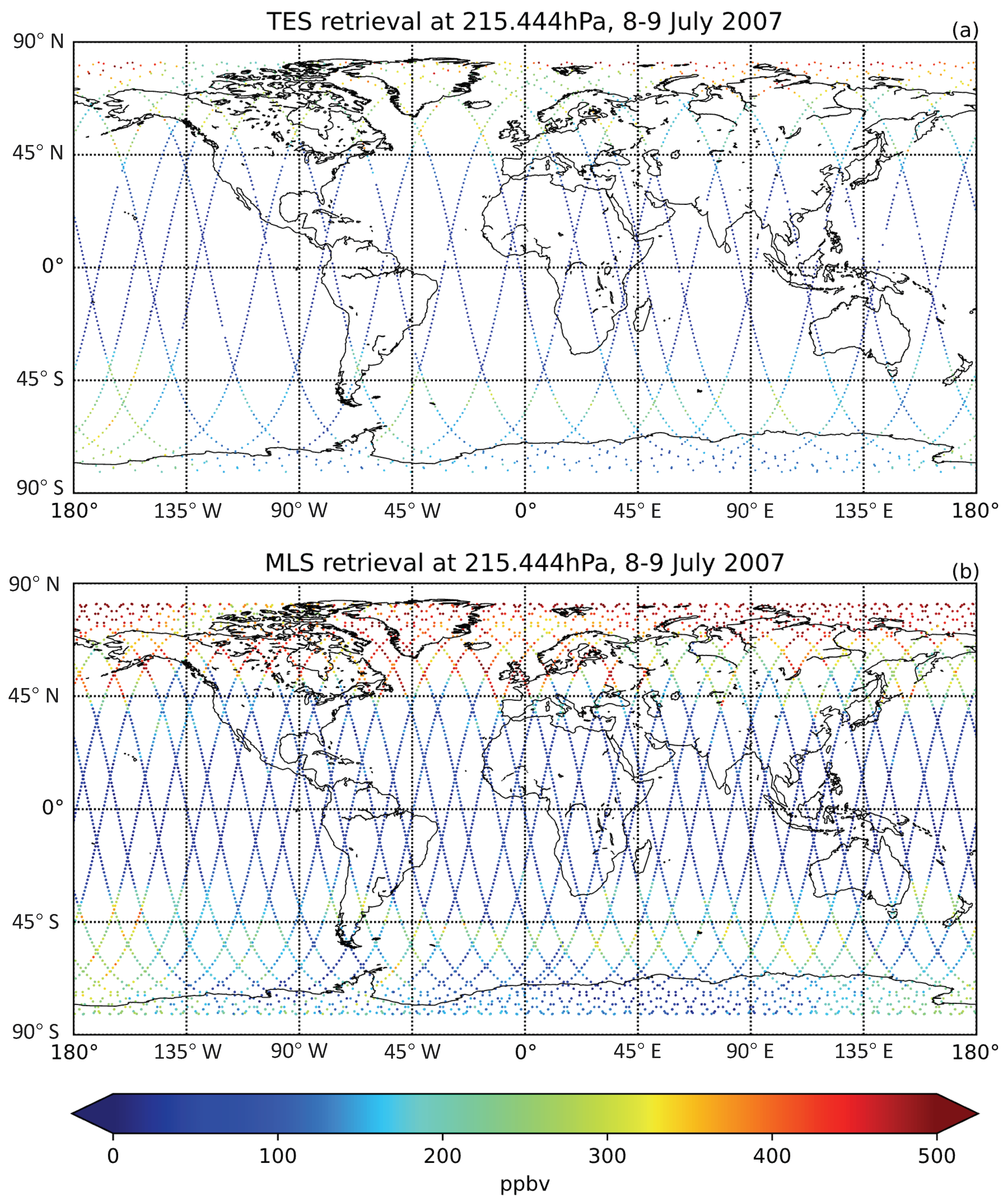
4.2. Horizonal Distribution of Combined Ozone at Specific Pressure Levels

In Figure 5, we present the comparisons of horizontal distribution of ozone among TES, MLS and combined product at 681.291 hPa (middle troposphere) and 215.444 hPa (upper troposphere) for 8–9 July 2007. The white dots in Figure 5c,f are the locations of combined ozone profiles. Interpolation is used in these figures for better illustration.

At 681.291 hPa, TES retrieval (Figure 5a) shows the variety and characteristic of ozone spatial distribution soundly. However, there are still some abnormal regions with extremely high ozone concentration such as northern Africa, the Arabian Peninsula and north-central Australia. This is probably caused by the dust reflection and absorption over the desert [56]. Compared with TES retrieval, MLS retrieval (Figure 5b) can hardly show any valuable information about the spatial distribution of ozone at this level since MLS is less sensitive in the lower troposphere. The combined product (Figure 5c) extracts most of the information from TES retrieval at this level. Aerosol plumes associated with biomass burning can reach into the free troposphere [59,60], which can be monitored by TES. Considering the combined product extracts the information from TES and is screened, it could be a better choice than TES product to monitor the biomass burning. Biomass combustion is a major source of trace gases including carbon monoxide (CO) in the atmosphere and has a great impact on tropospheric ozone formation [1,59,61]. The spatial distribution of the total sum of carbon emissions from 2000 to 2018 based on the Global Fire Emission Database (GFED) produced by Lin, Cohen [61] matches O₃ distribution patterns in Figure 5c nicely, especially in southern Africa, eastern Europe, northern Australia and Russia. This demonstrates the potential application of the combined product to monitor the biomass burning events.

At 215.444 hPa, ozone distribution from TES (Figure 5d) is similar to that of MLS (Figure 5e) in the middle to high latitudes in the Southern Hemisphere. However, in the Northern Hemisphere, the ozone concentration observed by TES is much lower than that by MLS in the middle to high latitude. Furthermore, TES ozone retrievals are lack of detail information in the low latitudes at this pressure level. Therefore, the combined product (Figure 5f), which contains most of information from MLS retrieval is a good choice at this level.

In addition, ozonesonde measurements from the WOUDC during 8–9 July 2007 are marked on the map in Figure 5 as colored squares with white edges (Table 1). At 681.291 hPa, the differences between ozonesonde measurements and three products are about the same. At 215.444 hPa, the differences between ozonesonde measurements and MLS product as well as combined product are obviously smaller than the difference between ozonesonde measurements and the TES product. However, these comparisons are very preliminary. The ozonesonde measurements are not many, all available measurements during these two days are presented here. There are large uncertainties when comparing the satellite-based observations to ozonesonde because they are not perfectly matched in location as we can see from the map in Figure 5. The two-day time window also increased the uncertainties for these comparisons. Furthermore, the uncertainties in spatial interpolation as well as ozonesonde measurements should also be considered.

4.3. Cases of Vertical Profile Validation

In this section, we present four examples of the validation results of the combined ozone vertical profile product. The first step is to match the time and position of the spaceborne and ground-based measurements. Then, the combined ozone profile is compared to the ozonesonde measurements.

The selected ozonesonde stations are Syowa station (39.6°E, 69°S), Sapporo station (141.3°E, 43.1°N) in Japan, and Ankara station (32.9°E, 40.0°N) in Turkish (Table 2). We select two of the closest TES-MLS pairs (pair A and B) to the measurement in Syowa station both in location and time, one (pair C) for Sapporo station and one (pair D) for Ankara station. Detailed information of the pairs is listed in Table 2.

The vertical profile comparisons of satellite retrievals and combined product with ozonesonde measurements are shown in Figure 6. The error profile of the combined product derived from TES and MLS precision data is also given (shown as red error bars), and the calculating process is described in the Supplementary Materials. For better demonstrations, we convert all profiles from MLS and TES to the same vertical pressure settings as the combined product, and then the null values in the upper stratosphere caused by original data deficiency (especially in ozonesonde and TES data) are removed. In general, the combined profile (red) follows the ozonesonde profile (black) closely at most of the pressure levels for all pairs (Figure 6a,d,g,j). To be more quantitatively, we use root mean square errors (RMSEs) to evaluate the performances of satellite profiles and combined profile as listed in

Table 3. RMSEs and MAREs of ozone profiles from satellites and ozonesonde. Unit: ppbv (RMSE), unitless (MARE).

	RMSE				MARE
	Combined	MLS	MLS a Priori	TES	Combined	MLS	MLS a Priori
Pair A	232.08	231.86	668.97	332.89	0.16	0.26	-
Pair B Pair C Pair D	288.47 453.60 315.24	288.61 454.62 312.17	733.35 772.59 199.13	451.72 915.07 904.27	0.18 0.43 0.20	0.29 0.42 0.21	- - 0.22

. Here, the RMSE is defined as,

$$\mathit{R}\mathit{M}\mathit{S}\mathit{E}=\sqrt{\frac{1}{\mathit{n}}{\displaystyle \mathrm{\sum }}_{\mathit{i}=1}^{\mathit{n}}{\left({\mathit{y}}_{\mathit{i}}^{\prime }-{\mathit{y}}_{\mathit{i}}\right)}^2}$$

(10)

where ${\mathit{y}}_{\mathit{i}}^{\prime }$ is the $\mathit{i}$-th element in the satellite or combined profile, ${\mathit{y}}_{\mathit{i}}$ is the $i$-th element in the ozonesonde profile, and $\mathit{n}$ is the number of the pressure levels of ozonesonde profile. The RMSEs of the combined profile and MLS profile are much smaller than those of the other two profiles in pair A, B and C, which indicates that the new combined profile and MLS profile match the ozonesonde better under this criterion. The RMSE of MLS a priori profile is the smallest in pair D, and those of the combined profile and MLS profile are also significantly smaller than that of TES, which means that MLS a priori profile, MLS profile and the combined profile represent ozonesonde relatively better than TES under such criterion. However, since the ozone volume mixing ratio in the upper atmosphere is much greater than that in the lower atmosphere, a slight deviation in the stratosphere may lead to a larger impact on RMSE than that in the lower troposphere, which means that the advantage of combined profile in the lower troposphere in pair D is covered up under such criterion. Therefore, we include mean absolute relative error (MARE) as a second criterion, which are also listed in Table 3. Here, the MARE is defined as,

$$\mathit{M}\mathit{A}\mathit{R}\mathit{E}=\frac{1}{\mathit{n}}{{\displaystyle \mathrm{\sum }}}_{\mathit{i}=1}^{\mathit{n}}\left|\frac{{\mathit{y}}_{\mathit{i}}^{\prime }-{\mathit{y}}_{\mathit{i}}}{{\mathit{y}}_{\mathit{i}}}\right|.$$

(11)

MARE is unaffected by the difference in order of magnitude between stratosphere and troposphere, thus the advantage of combined profile over MLS profile is much more obvious under this criterion as shown in pair A and B (Table 3). In pair C and D, the MARE of the combined profile is almost the same as those of MLS profile and MLS a priori profile (in pair D), which may be caused by the observation uncertainty and the sampling bias of combined profiles and ozonesonde measurements in location and time. Based on validation results with these two criteria, the superiority of the combined profile is demonstrated quantitatively. The combined profile shows an outstanding general performance in presenting vertical ozone distribution.

We also calculate the RMSEs for different vertical regions as listed in

Table 4. RMSEs of ozone profiles from satellites and ozonesonde in lower troposphere (below 500 hPa), upper troposphere (500–100 hPa) and stratosphere (above 100 hPa). Unit: ppbv.

	RMSE
	Lower Troposphere				Upper Troposphere				Stratosphere
	Combined	MLS	MLS a Priori	TES	Combined	MLS	MLS a Priori	TES	Combined	MLS	MLS a Priori	TES
Pair A	2.74	10.56	10.10	2.66	82.27	81.26	160.27	120.66	314.88	314.70	918.58	451.20
Pair B	1.96	11.92	11.41	1.93	89.07	87.76	164.39	112.52	389.41	389.76	997.92	613.41
Pair C	19.02	17.62	18.44	19.00	86.44	86.73	215.58	140.63	631.72	633.13	1068.78	1277.15
Pair D	4.76	8.04	8.77	4.73	86.67	85.56	57.71	43.77	431.49	427.31	272.13	1253.50

to avoid the interference from the difference in order of magnitude. In lower troposphere, the RMSEs of the combined profile and the TES profile are much smaller than those of other profiles in most cases (Pair A, B and D). In upper troposphere and stratosphere, the RMSEs of combined profile and MLS profile are much smaller than those of other profiles in most cases (Pair A, B and C) as well. Therefore, the general advantage of combined profiles in all these three regions is demonstrated under this criterion.

5. Conclusions

The vertical profile of ozone is of great significance for researchers to know about the ozone distribution in the atmosphere. TES and MLS retrieved data provide us with a considerable amount of vertical information of ozone. Still, its quality is partly limited by the poor sensitivity of the instruments in certain pressure levels. In this study, we derive an algorithm of combining vertical ozone profile from TES and MLS level 2 retrieved data. Compared with other combining methods, our method is less resource-consuming in computing process and is easier to generalize to other chemical species. Theoretically, our algorithm can be applied to chemical species observed from both MLS and TES, such as CO, CH₃OH, HCN, N₂O, and also species retrievals by other satellite instruments with similar expressions.

The vertical profile and horizontal distribution indicate that the combined product extracts weighted information from TES and MLS in both troposphere and stratosphere based on the averaging kernels of MLS. Validation of the pairs also indicates that the combined products match better to ozonesonde measurements than MLS or TES products alone in general under the quantitative criteria of RMSE and MARE.

The combined product will help researchers with studies related to the distribution of ozone, especially in the area of ozone exchange between different pressure levels since ozone data with uniformity of pressure levels and coincidence of space and time is indispensable to this research area.

In our future work, we will try to take the impact of scattering geometries into account for further improvement of our algorithm considering the different view angles of MLS and TES. The scattering geometries of observation instruments can not only affect the retrieval of the properties of aerosol and cloud [62,63,64], but also the retrieval of trace gases. For MLS, the long view path length due to its limb sounding leads to enhancement of the signature of trace gases in the observed spectra [65], and the limb scanning also offers better vertical resolution but worse horizontal resolution than nadir observations [65,66]. Furthermore, microwave signals are unaffected by aerosol, whose angle-dependent scattering effect can hamper observations at shorter wavelength such as near infrared [65,67,68,69,70]. For TES, the nadir observation offers better horizontal resolution [65,66]. Thus, we can add parameter related to the scattering geometries of MLS and TES to the combination algorithm to adjust the weight of each profile to meet the requirements of different observation conditions and spatial resolutions.

References

1. Seinfeld, J.H.P.; Spyros, N. Atmospheric Chemistry and Physics: From Air Pollution to Climate Change, 3rd ed.; Wiley: New York, NY, USA, 2016. [Google Scholar]
2. Haagen-Smit, A.J. Chemistry and Physiology of Los Angeles Smog. Ind. Eng. Chem. 1952, 44, 1342–1346. [Google Scholar] [CrossRef]
3. Jones, A.E.; Anderson, P.S.; Wolff, E.W.; Roscoe, H.K.; Marshall, G.J.; Richter, A.; Brough, N.; Colwell, S.R. Vertical structure of Antarctic tropospheric ozone depletion events: Characteristics and broader implications. Atmos. Chem. Phys. 2010, 10, 7775–7794. [Google Scholar] [CrossRef] [Green Version]
4. Liu, X.; Bhartia, P.K.; Chance, K.; Spurr, R.J.D.; Kurosu, T.P. Ozone profile retrievals from the Ozone Monitoring Instrument. Atmos. Chem. Phys. 2010, 10, 2521–2537. [Google Scholar] [CrossRef] [Green Version]
5. Barré, J.; Peuch, V.-H.; Attié, J.-L.; El Amraoui, L.; Lahoz, W.A.; Josse, B.; Claeyman, M.; Nédélec, P. Stratosphere-troposphere ozone exchange from high resolution MLS ozone analyses. Atmos. Chem. Phys. 2012, 12, 6129–6144. [Google Scholar] [CrossRef] [Green Version]
6. Wargan, K.; Pawson, S.; Stajner, I.; Thouret, V. Spatial structure of assimilated ozone in the upper troposphere and lower stratosphere. J. Geophys. Res. Atmos. 2010, 115, D24316. [Google Scholar] [CrossRef]
7. Semane, N.; Peuch, V.-H.; El Amraoui, L.; Bencherif, H.; Massart, S.; Cariolle, D.; Attié, J.-L.; Abida, R. An observed and analysed stratospheric ozone intrusion over the high Canadian Arctic UTLS region during the summer of 2003. Q. J. R. Meteorol. Soc. 2007, 133, 171–178. [Google Scholar] [CrossRef]
8. Stajner, I.; Wargan, K.; Pawson, S.; Hayashi, H.; Chang, L.-P.; Hudman, R.C.; Froidevaux, L.; Livesey, N.; Levelt, P.F.; Thompson, A.M.; et al. Assimilated ozone from EOS-Aura: Evaluation of the tropopause region and tropospheric columns. J. Geophys. Res. 2008, 113, D16. [Google Scholar] [CrossRef] [Green Version]
9. El Amraoui, L.; Attié, J.-L.; Semane, N.; Claeyman, M.; Peuch, V.-H.; Warner, J.; Ricaud, P.; Cammas, J.-P.; Piacentini, A.; Josse, B.; et al. Midlatitude stratosphere–troposphere exchange as diagnosed by MLS O3 and MOPITT CO assimilated fields. Atmos. Chem. Phys. 2010, 10, 2175–2194. [Google Scholar] [CrossRef] [Green Version]
10. Megie, G.J.; Ancellet, G.; Pelon, J. Lidar measurements of ozone vertical profiles. Appl. Opt. 1985, 24, 3454–3463. [Google Scholar] [CrossRef] [Green Version]
11. Chi, X.; Liu, C.; Xie, Z.; Fan, G.; Wang, Y.; He, P.; Fan, S.; Hong, Q.; Wang, Z.; Yu, X.; et al. Observations of ozone vertical profiles and corresponding precursors in the low troposphere in Beijing, China. Atmos. Res. 2018, 213, 224–235. [Google Scholar] [CrossRef]
12. Komhyr, W.D. Electrical concentration cells for gas analysis. Ann. Geophys. 1969, 25, 203–210. [Google Scholar]
13. Komhyr, W.D.; Barnes, R.A.; Brothers, G.B.; Lathrop, J.A.; Opperman, D.P. Electrochemical concentration cell ozonesonde performance evaluation during STOIC 1989. J. Geophys. Res. Atmos. 1995, 100, 9231–9244. [Google Scholar] [CrossRef]
14. Jonson, J.E.; Stohl, A.; Fiore, A.M.; Hess, P.; Szopa, S.; Wild, O.; Zeng, G.; Dentener, F.J.; Lupu, A.; Schultz, M.G.; et al. A multi-model analysis of vertical ozone profiles. Atmos. Chem. Phys. 2010, 10, 5759–5783. [Google Scholar] [CrossRef] [Green Version]
15. Newchurch, M.J.; Ayoub, M.A.; Oltmans, S.; Johnson, B.; Schmidlin, F.J. Vertical distribution of ozone at four sites in the United States. J. Geophys. Res. 2003, 108, ACH 9-1–ACH 9-17. [Google Scholar] [CrossRef]
16. Russell III, J.M.; Gordley, L.L.; Park, J.H.; Drayson, S.R.; Hesketh, W.D.; Cicerone, R.J.; Tuck, A.F.; Frederick, J.E.; Harries, J.E.; Crutzen, P.J. The halogen occultation experiment. J. Geophys. Res. Atmos. 1993, 98, 10777–10797. [Google Scholar] [CrossRef]
17. Roche, A.; Kumer, J.; Mergenthaler, J.; Ely, G.; Uplinger, W.; Potter, J.; James, T.; Sterritt, L. The cryogenic limb array etalon spectrometer (CLAES) on UARS: Experiment description and performance. J. Geophys. Res. Atmos. 1993, 98, 10763–10775. [Google Scholar] [CrossRef]
18. Connor, B.J.; Scheuer, C.; Chu, D.; Remedios, J.; Grainger, R.; Rodgers, C.; Taylor, F. Ozone in the middle atmosphere as measured by the improved stratospheric and mesospheric sounder. J. Geophys. Res. Atmos. 1996, 101, 9831–9841. [Google Scholar] [CrossRef]
19. Barath, F.; Chavez, M.; Cofield, R.; Flower, D.; Frerking, M.; Gram, M.; Harris, W.; Holden, J.; Jarnot, R.; Kloezeman, W. The upper atmosphere research satellite microwave limb sounder instrument. J. Geophys. Res. Atmos. 1993, 98, 10751–10762. [Google Scholar] [CrossRef]
20. Llewellyn, E.; Lloyd, N.; Degenstein, D.; Gattinger, R.; Petelina, S.; Bourassa, A.; Wiensz, J.; Ivanov, E.; McDade, I.; Solheim, B. The OSIRIS instrument on the Odin spacecraft. Can. J. Phys. 2004, 82, 411–422. [Google Scholar] [CrossRef]
21. Fischer, H.; Birk, M.; Blom, C.; Carli, B.; Carlotti, M.; Von Clarmann, T.; Delbouille, L.; Dudhia, A.; Ehhalt, D.; Endemann, M. MIPAS: An instrument for atmospheric and climate research. Atmos. Chem. Phys. 2008, 8, 2151–2188. [Google Scholar] [CrossRef] [Green Version]
22. Kyrölä, E.; Tamminen, J.; Leppelmeier, G.; Sofieva, V.; Hassinen, S.; Bertaux, J.; Hauchecorne, A.; Dalaudier, F.; Cot, C.; Korablev, O. GOMOS on Envisat: An overview. Adv. Space Res. 2004, 33, 1020–1028. [Google Scholar] [CrossRef]
23. Burrows, J.; Hölzle, E.; Goede, A.; Visser, H.; Fricke, W. SCIAMACHY—Scanning imaging absorption spectrometer for atmospheric chartography. Acta Astronaut. 1995, 35, 445–451. [Google Scholar] [CrossRef]
24. Pagano, T.S.P.; Vivienne, H. The Atmospheric Infrared Sounder. In Handbook of Air Quality and Climate Change; Springer: Singapore, 2022. [Google Scholar] [CrossRef]
25. Levelt, P.F.; Van Den Oord, G.H.; Dobber, M.R.; Malkki, A.; Visser, H.; De Vries, J.; Stammes, P.; Lundell, J.O.; Saari, H. The ozone monitoring instrument. IEEE Trans. Geosci. Remote Sens. 2006, 44, 1093–1101. [Google Scholar] [CrossRef]
26. Gille, J.C.; Barnett, J.J.; Whitney, J.G.; Dials, M.A.; Woodard, D.; Rudolf, W.P.; Lambert, A.; Mankin, W. The High-Resolution Dynamics Limb Sounder (HIRDLS) experiment on AURA. In Proceedings of the Optical Science and Technology, SPIE’s 48th Annual Meeting, San Diego, CA, USA, 3 August 2003; pp. 162–171. [Google Scholar]
27. Waters, J.W.; Froidevaux, L.; Harwood, R.S.; Jarnot, R.F.; Pickett, H.M.; Read, W.G.; Siegel, P.H.; Cofield, R.E.; Filipiak, M.J.; Flower, D.A. The earth observing system microwave limb sounder (EOS MLS) on the Aura satellite. IEEE Trans. Geosci. Remote Sens. 2006, 44, 1075–1092. [Google Scholar] [CrossRef]
28. Beer, R.; Glavich, T.A.; Rider, D.M. Tropospheric Emission Spectrometer for the Earth Observing System’s Aura satellite. Appl. Opt. 2001, 40, 2356–2367. [Google Scholar] [CrossRef]
29. Mauldin III, L.; Zaun, N.; McCormick, M., Jr.; Guy, J.; Vaughn, W. Stratospheric Aerosol and Gas Experiment II instrument: A functional description. Opt. Eng. 1985, 24, 307–312. [Google Scholar] [CrossRef]
30. Thomason, L.W.; Chu, W.P.; Pitts, M.C. Stratospheric Aerosol and Gas Experiment III. In Satellite Remote Sensing of Clouds and the Atmosphere III; International Society for Optics and Photonics: Bellingham, WA, USA, 1998; pp. 286–291. [Google Scholar]
31. Tan, S.-Y. NOAA Satellites and Solar Backscatter Ultra Violet (SBUV) Subsystems. In Handbook of Cosmic Hazards and Planetary Defense; Springer: Cham, The Netherlands, 2015. [Google Scholar] [CrossRef]
32. De Laat, A.T.J.; van Weele, M. The 2010 Antarctic ozone hole: Observed reduction in ozone destruction by minor sudden stratospheric warmings. Sci. Rep. 2011, 1, 38. [Google Scholar] [CrossRef] [Green Version]
33. Ziemke, J.R.; Chandra, S.; Labow, G.J.; Bhartia, P.K.; Froidevaux, L.; Witte, J.C. A global climatology of tropospheric and stratospheric ozone derived from Aura OMI and MLS measurements. Atmos. Chem. Phys. 2011, 11, 9237–9251. [Google Scholar] [CrossRef] [Green Version]
34. McPeters, R.D.; Labow, G.J. Climatology 2011: An MLS and sonde derived ozone climatology for satellite retrieval algorithms. J. Geophys. Res. Atmos. 2012, 117, D17. [Google Scholar] [CrossRef] [Green Version]
35. Labow, G.J.; Ziemke, J.R.; McPeters, R.D.; Haffner, D.P.; Bhartia, P.K. A total ozone-dependent ozone profile climatology based on ozonesondes and Aura MLS data. J. Geophys. Res. Atmos. 2015, 120, 2537–2545. [Google Scholar] [CrossRef]
36. Shine, K.P.; Fouquart, Y.; Ramaswamy, V.; Solomon, S.; Srinivasan, J. Climate Change 1995: The Science of Climate Change: Contribution of Working Group I to the Second Assessment Report of the Intergovernmental Panel on Climate Change; Section 2.4; Cambridge University Press: Cambridge, UK, 1996. [Google Scholar]
37. Ziemke, J.R.; Olsen, M.A.; Witte, J.C.; Douglass, A.R.; Strahan, S.E.; Wargan, K.; Liu, X.; Schoeberl, M.R.; Yang, K.; Kaplan, T.B.; et al. Assessment and applications of NASA ozone data products derived from Aura OMI/MLS satellite measurements in context of the GMI chemical transport model. J. Geophys. Res. Atmos. 2014, 119, 5671–5699. [Google Scholar] [CrossRef]
38. Jourdain, L.; Worden, H.M.; Worden, J.R.; Bowman, K.; Li, Q.; Eldering, A.; Kulawik, S.S.; Osterman, G.; Boersma, K.F.; Fisher, B.; et al. Tropospheric vertical distribution of tropical Atlantic ozone observed by TES during the northern African biomass burning season. Geophys. Res. Lett. 2007, 34, 28284. [Google Scholar] [CrossRef] [Green Version]
39. Zhang, L.; Jacob, D.J.; Bowman, K.W.; Logan, J.A.; Turquety, S.; Hudman, R.C.; Li, Q.; Beer, R.; Worden, H.M.; Worden, J.R.; et al. Ozone-CO correlations determined by the TES satellite instrument in continental outflow regions. Geophys. Res. Lett. 2006, 33, 26399. [Google Scholar] [CrossRef] [Green Version]
40. Jourdain, L.; Kulawik, S.S.; Worden, H.M.; Pickering, K.E.; Worden, J.; Thompson, A.M. Lightning NOx emissions over the USA constrained by TES ozone observations and the GEOS-Chem model. Atmos. Chem. Phys. 2010, 10, 107–119. [Google Scholar] [CrossRef] [Green Version]
41. Sun, W.; Hess, P.; Tian, B. The response of the equatorial tropospheric ozone to the Madden–Julian Oscillation in TES satellite observations and CAM-chem model simulation. Atmos. Chem. Phys. 2014, 14, 11775–11790. [Google Scholar] [CrossRef] [Green Version]
42. Miyazaki, K.; Eskes, H.J.; Sudo, K.; Takigawa, M.; van Weele, M.; Boersma, K.F. Simultaneous assimilation of satellite NO2, O3, CO, and HNO3 data for the analysis of tropospheric chemical composition and emissions. Atmos. Chem. Phys. 2012, 12, 9545–9579. [Google Scholar] [CrossRef] [Green Version]
43. Miyazaki, K.; Eskes, H.J.; Sudo, K. A tropospheric chemistry reanalysis for the years 2005–2012 based on an assimilation of OMI, MLS, TES, and MOPITT satellite data. Atmos. Chem. Phys. 2015, 15, 8315–8348. [Google Scholar] [CrossRef] [Green Version]
44. Warner, J.X.; Yang, R.; Wei, Z.; Carminati, F.; Tangborn, A.; Sun, Z.; Lahoz, W.; Attié, J.-L.; El Amraoui, L.; Duncan, B. Global carbon monoxide products from combined AIRS, TES and MLS measurements on A-train satellites. Atmos. Chem. Phys. 2014, 14, 103–114. [Google Scholar] [CrossRef] [Green Version]
45. Rodgers, C.D. Inverse Methods for Atmospheric Sounding: Theory and Practice; World Scientific: Singapore, 2000; Volume 2. [Google Scholar]
46. Fu, D.; Worden, J.R.; Liu, X.; Kulawik, S.S.; Bowman, K.W.; Natraj, V. Characterization of ozone profiles derived from Aura TES and OMI radiances. Atmos. Chem. Phys. 2013, 13, 3445–3462. [Google Scholar] [CrossRef] [Green Version]
47. Luo, M.; Read, W.; Kulawik, S.; Worden, J.; Livesey, N.; Bowman, K.; Herman, R. Carbon monoxide (CO) vertical profiles derived from joined TES and MLS measurements. J. Geophys. Res. Atmos. 2013, 118, 10601–610613. [Google Scholar] [CrossRef] [Green Version]
48. Fu, D.; Kulawik, S.S.; Miyazaki, K.; Bowman, K.W.; Worden, J.R.; Eldering, A.; Livesey, N.J.; Teixeira, J.; Irion, F.W.; Herman, R.L.; et al. Retrievals of tropospheric ozone profiles from the synergism of AIRS and OMI: Methodology and validation. Atmos. Meas. Tech. 2018, 11, 5587–5605. [Google Scholar] [CrossRef] [Green Version]
49. Beer, R.; Bowman, K.W.; Brown, P.D.; Clough, S.A.; Eldering, A.; Goldman, A.; Jacob, D.J.; Lampel, M.; Logan, J.A.; Luo, M.; et al. Tropospheric Emission Spectrometer (TES) Level 2 Algorithm Theoretical Basis Document, version 1.15; Jet Propulsion Laboratory, California Institute of Technology: Pasadena, CA, USA, 2002. [Google Scholar]
50. Waymark, C.; Dudhia, A.; Barnett, J.; Taylor, F.; Piccolo, C. Combined ozone retrieval using the Michelson Interferometer for Passive Atmospheric Sounding (MIPAS) and the Tropospheric Emission Spectrometer (TES). In Proceedings of the Envisat Symposium 2007, Montreux, Switzerland, 23–27 April 2007. [Google Scholar]
51. Schoeberl, M.R.; Douglass, A.R.; Hilsenrath, E.; Bhartia, P.K.; Beer, R.; Waters, J.W.; Gunson, M.R.; Froidevaux, L.; Gille, J.C.; Barnett, J.J.; et al. Overview of the EOS Aura mission. IEEE Trans. Geosci. Remote Sens. 2006, 44, 1066–1074. [Google Scholar] [CrossRef] [Green Version]
52. Beer, R. TES on the Aura mission: Scientific objectives, measurements, and analysis overview. IEEE Trans. Geosci. Remote Sens. 2006, 44, 1102–1105. [Google Scholar] [CrossRef]
53. Livesey, N.J.; Read, W.G.; Wagner, P.A.; Froidevaux, L.; Santee, M.L.; Schwartz, M.J.; Lambert, A.; Valle, L.F.M.; Pumphrey, H.C.; Manney, G.L.; et al. Earth Observing System (EOS) Aura Microwave Limb Sounder (MLS) Version 5.0× Level 2 and 3 Data Quality and Description Document, Version 5.0–1.0a; JPL D-105336; California Institute of Technology: Pasadena, CA, USA, 2020. [Google Scholar]
54. Livesey, N.J.; Van Snyder, W.; Read, W.G.; Wagner, P.A. Retrieval algorithms for the EOS Microwave Limb Sounder (MLS). IEEE Trans. Geosci. Remote Sens. 2006, 44, 1144–1155. [Google Scholar] [CrossRef]
55. Deshler, T.; Mercer, J.L.; Smit, H.G.J.; Stubi, R.; Levrat, G.; Johnson, B.J.; Oltmans, S.J.; Kivi, R.; Thompson, A.M.; Witte, J.; et al. Atmospheric comparison of electrochemical cell ozonesondes from different manufacturers, and with different cathode solution strengths: The Balloon Experiment on Standards for Ozonesondes. J. Geophys. Res. 2008, 113, 8975. [Google Scholar] [CrossRef]
56. Bowman, K.; Cady-Pereira, K.; Eldering, A.F.; Brendan, F.D.; Herman, R.J.D.; Jourdain, L.; Kulawik, S.; Luo, M.; Monarrez, R.O.; Gregory, P.; et al. Earth Observating System (EOS) Tropospheric Emission Spectrometer (TES) Level 2 (L2) Data User’s Guide, Version 8.0.; JPL D-38042; California Institute of Technology: Pasadena, CA, USA, 2020. [Google Scholar]
57. Rodgers, C.D.; Connor, B.J. Intercomparison of remote sounding instruments. J. Geophys. Res. Atmos. 2003, 108, 2299. [Google Scholar] [CrossRef] [Green Version]
58. Luo, M.; Rinsland, C.P.; Rodgers, C.D.; Logan, J.A.; Worden, H.; Kulawik, S.; Eldering, A.; Goldman, A.; Shephard, M.W.; Gunson, M.; et al. Comparison of carbon monoxide measurements by TES and MOPITT: Influence of a priori data and instrument characteristics on nadir atmospheric species retrievals. J. Geophys. Res. 2007, 112, 7663. [Google Scholar] [CrossRef] [Green Version]
59. Wang, S.; Cohen, J.B.; Lin, C.; Deng, W. Constraining the relationships between aerosol height, aerosol optical depth and total column trace gas measurements using remote sensing and models. Atmos. Chem. Phys. 2020, 20, 15401–15426. [Google Scholar] [CrossRef]
60. Wang, S.; Cohen, J.B.; Deng, W.; Qin, K.; Guo, J. Using a New Top-Down Constrained Emissions Inventory to Attribute the Previously Unknown Source of Extreme Aerosol Loadings Observed Annually in the Monsoon Asia Free Troposphere. Earth’s Future 2021, 9, e2021EF002167. [Google Scholar] [CrossRef]
61. Lin, C.; Cohen, J.B.; Wang, S.; Lan, R.; Deng, W. A new perspective on the spatial, temporal, and vertical distribution of biomass burning: Quantifying a significant increase in CO emissions. Environ. Res. Lett. 2020, 15, 104091. [Google Scholar] [CrossRef]
62. Kalashnikova, O.V.; Garay, M.J.; Martonchik, J.V.; Diner, D.J. MISR Dark Water aerosol retrievals: Operational algorithm sensitivity to particle non-sphericity. Atmos. Meas. Tech. 2013, 6, 24. [Google Scholar] [CrossRef] [Green Version]
63. Wang, Y.; Yang, P.; King, M.D.; Baum, B.A. Optical Property Model for Cirrus Clouds Based on Airborne Multi-Angle Polarization Observations. Remote Sens. 2021, 13, 2754. [Google Scholar] [CrossRef]
64. Liang, L.; Di Girolamo, L. A global analysis on the view-angle dependence of plane-parallel oceanic liquid water cloud optical thickness using data synergy from MISR and MODIS. J. Geophys. Res. Atmos. 2013, 118, 15. [Google Scholar] [CrossRef]
65. Kunzi, K.; Bauer, P.; Eresmaa, R.; Eriksson, P.; Healy, S.B.; Mugnai, A.; Livesey, N.; Prigent, C.; Smith, E.A.; Stephens, G. Microwave absorption, emission and scattering: Trace gases and meteorological parameters. In The Remote Sensing of Tropospheric Composition from Space; Springer: Berlin/Heidelberg, Germany, 2011; pp. 153–230. [Google Scholar]
66. Rosenkranz, P.W.; Hutchison, K.D.; Hardy, K.R.; Davis, M.S. An assessment of the impact of satellite microwave sounder incidence angle and scan geometry on the accuracy of atmospheric temperature profile retrievals. J. Atmos. Ocean. Technol. 1997, 14, 488–494. [Google Scholar] [CrossRef]
67. Zeng, Z.-C.; Xu, F.; Natraj, V.; Pongetti, T.J.; Shia, R.-L.; Zhang, Q.; Sander, S.P.; Yung, Y.L. Remote sensing of angular scattering effect of aerosols in a North American megacity. Remote Sens. Environ. 2020, 242, 111760. [Google Scholar] [CrossRef] [Green Version]
68. Aben, I.; Hasekamp, O.; Hartmann, W. Uncertainties in the space-based measurements of CO2 columns due to scattering in the Earth’s atmosphere. J. Quant. Spectrosc. Radiat. Transf. 2007, 104, 450–459. [Google Scholar] [CrossRef]
69. Yoshida, Y.; Ota, Y.; Eguchi, N.; Kikuchi, N.; Nobuta, K.; Tran, H.; Morino, I.; Yokota, T. Retrieval algorithm for CO2 and CH4 column abundances from short-wavelength infrared spectral observations by the Greenhouse gases observing satellite. Atmos. Meas. Tech. 2011, 4, 717–734. [Google Scholar] [CrossRef] [Green Version]
70. O’Dell, C.W.; Connor, B.; Bösch, H.; O’Brien, D.; Frankenberg, C.; Castano, R.; Christi, M.; Eldering, D.; Fisher, B.; Gunson, M.; et al. The ACOS CO2 retrieval algorithm–Part 1: Description and validation against synthetic observations. Atmos. Meas. Tech. 2012, 5, 99–121. [Google Scholar] [CrossRef] [Green Version]
Figure 1. The orbit footprints and corresponding ozone volume mixing ratio from TES retrieval (a) and MLS retrieval (b) on 8–9 July 2007.
Remotesensing 14 01588 g001
Figure 2. The pairing result of TES locations (blue) and MLS locations (red) on 8–9 July 2007.
Remotesensing 14 01588 g002
Figure 3. Vertical averaging kernels of (a) MLS ozone and (b) TES ozone at 70°N. (c) The partial enlargement of (b) between 1000 hPa and 50 hPa.
Remotesensing 14 01588 g003
Figure 4. Comparison among ozone vertical profiles of combined profiles (red), MLS profiles (blue), TES profiles (green), and MLS a priori profiles (yellow) at (a) (116°E, 0°), (b) (39°E, 35°N) and (c) (19°E, 70°N).
Remotesensing 14 01588 g004
Figure 5. Comparison among horizontal distributions (interpolated) of ozone at 681.291 hPa (ac) and 215.444 hPa (df) for 8–9 July 2007: (a,d) TES product, (b,e) MLS product, and (c,f) combined product. Locations corresponding to each product are marked by white dots. Colored squares with white edges are ozonesonde measurements.
Remotesensing 14 01588 g005
Figure 6. Comparison among vertical profiles for validation for (a) pair A, (d) pair B, (g) pair B, and (j) pair B: combined profile with error bars (red), MLS profile (blue), TES profile (green), MLS a priori profile (yellow), and ozonesonde profile (black). (b) The partial enlargement of (a) between 35 hPa and 5 hPa. (c) The partial enlargement of (a) between 900 hPa and 350 hPa. (e) Similar as (b), but for pair B. (f) Similar as (c), but for pair B. (h) The partial enlargement of (g) between 40 hPa and 5 hPa. (i) The partial enlargement of (g) between 1050 hPa and 350 hPa. (k) The partial enlargement of (j) between 40 hPa and 5 hPa. (l) The partial enlargement of (j) between 900 hPa and 350 hPa.
Remotesensing 14 01588 g006