An Approach for Predicting Global Ionospheric TEC Using Machine Learning

Abstract

Accurate corrections for ionospheric total electron content (TEC) and early warning information are crucial for global navigation satellite system (GNSS) applications under the influence of space weather. In this study, we propose to use a new machine learning model—the Prophet model, to predict the global ionospheric TEC by establishing a short-term ionospheric prediction model. We use 15th-order spherical harmonic coefficients provided by the Center for Orbit Determination in Europe (CODE) as the training data set. Historical spherical harmonic coefficient data from 7 days, 15 days, and 30 days are used as the training set to model and predict 256 spherical harmonic coefficients. We use the predicted coefficients to generate a global ionospheric TEC forecast map based on the spherical harmonic function model and select a year with low solar activity (63.4 < F10.7 < 81.8) and a year with the high solar activity (79.5 < F10.7 < 255.0) to carry out a sliding 2-day forecast experiment. Meanwhile, we verify the model performance by comparing the forecasting results with the CODE forecast product (COPG) and final product (CODG). The results show that we obtain the best predictions by using 15 days of historical data as the training set. Compared with the results of CODE’S 1-Day (C1PG) and CODE’S 2-Day (C2PG). The number of days with RMSE better than COPG on the first and second day of the low-solar-activity year is 151 and 158 days, respectively. This statistic for high-solar-activity year is 183 days and 135 days.

1. Introduction

The state of the Earth’s ionosphere always affects the accuracy and reliability of global navigation satellite system (GNSS) positioning, navigation, and timing [1,2,3]. For low latitudes, equatorial ionization anomaly and equatorial plasma bubbles are two major phenomena [4,5]. For mid-latitude, mid-latitude enhancement is a typical phenomenon [6]. For high-latitude, tongue of ionization is a typical phenomenon [7]. Meanwhile, earthquakes and other natural disasters have an impact on causing ionospheric anomalies [8,9]. These phenomena of ionosphere play major roles in GNSS positioning, navigation, and timing. The ionospheric total electron content (TEC) is the total number of electrons in the column between the satellite and the receiver from the top to the bottom of the ionosphere. This number directly determines the time delay for a satellite signal to pass through the ionosphere. In real-time precision positioning, high accurate ionospheric prediction models play a vital role in positioning accuracy and accelerating the positioning convergence [10,11]. Monitoring the inversion of the ionosphere using GNSS is a feasible method [12,13]. Therefore, the tasks of monitoring and forecasting the ionosphere and building a high-precision ionosphere prediction model have important research value.

For this largest naturally occurring error source for GNSS [14], broadcasting or empirical models of the ionosphere are most commonly used to correct for ionospheric delay, such as the Klobuchar model [15,16,17], the NeQuick model [18], the BDGIM [19] and the International Reference Ionosphere (IRI) model [20,21]. These models can reach a forecast accuracy of approximately 50~75% [15,18], and meet user needs in terms of single-frequency high-precision positioning [22,23]. However, they are susceptible to accuracy limiting factors such as solar activity and sudden changes in the Earth’s environment. In 1998, the International GNSS Service (IGS) established an ionospheric working group to regularly publish precision GNSS products, which provide a wealth of research data for ionospheric research [24,25,26]. At present, the main institutions providing ionospheric prediction products are the Center for Orbit Determination in Europe (CODE), the European Space Agency (ESA), and the Universitat Politècnica de Catalunya (UPC) in Spain. CODE and ESA provide ionospheric prediction products one day and two days in advance, while UPC provides ionospheric prediction products two days in advance [27,28].

In recent years, many ionospheric researchers have conducted a series of short-term forecasting studies and developed ionospheric products with higher accuracy than empirical ionospheric models to make full use of historical data to analyze and extract the characteristics of ionospheric TEC changes. Tulunay et al. [29] developed the Middle East Technical University Neural Network (METU-NN) model, composed of a hidden layer and multiple neurons, to predict ionospheric TEC maps over Europe. Xia et al. [30] used support vector machine (SVM) and graphics acceleration technology to establish an ionospheric forecasting model for China. Zhukov et al. [31,32] established a regional ionospheric forecasting model based on machine learning methods such as random forest, support vector regression, and gradient boosting. Then they used geomagnetic activity index and solar activity index driven model and created a global ionospheric total electron content model, which both have higher performances compared with NeQuick2, Klobuchar and GEMTEC models. Huang et al. [33] developed a single short-term ionospheric TEC prediction model based on a radial basis function (RBF) neural network. Lee et al. [34] generated global ionospheric TEC forecasts based on a generative countermeasure network. Srivani et al. [35] established a long short-term memory (LSTM) neural network prediction model using observation data from Bengaluru Station in India. Ruwali et al. [36] introduced the application of LSTM, gated recurrent unit (GRU), and convolutional neural network (CNN)-LSTM networks in the field of ionospheric prediction, and experiments showed that the CNN-LSTM network had the best prediction effect.

Li et al. [37] used an indirect forecasting method based on spherical harmonic function coefficients provided by the IGS and an autoregressive and moving average (ARMA) model to realize global ionospheric TEC forecasting. Wang et al. [38] used an adaptive autoregressive model and a spherical harmonic function model to predict the global ionospheric map (GIM). Wang et al. [39] and Qiu et al. [40] used a semiautomatic kernel estimation method and an improved variant thereof, respectively, to predict the spherical harmonic function coefficients provided by CODE. They introduced a 15th-order spherical harmonic function coefficient model to establish a version of CODE’S 1-Day Predicted GIM (C1PG) with higher model longitudes. Liu et al. [41] input four factors—the historical sequence of the spherical harmonic coefficients, the solar extreme ultraviolet (EUV) flux, the disturbance storm time (Dst) index, and the hour of the day—into the LSTM neural network to predict the generation of spherical harmonic coefficients in periods of magnetic storms and magnetic quiet periods. The GIM was obtained using a forecasting model with higher accuracy than IRI-2016 or NeQuick-2.

However, understanding ways to improve the forecasting accuracy of global ionospheric model is still a key issue worthy of in-depth discussion due to the changeable and sensitive ionospheric state affected by many factors, such as solar, the earth’s magnetic field, electric field, etc. In this study, we propose to use a new machine learning model—the Prophet model—to predict the global ionospheric TEC. We use 15th-order spherical harmonic function coefficients to forecast and generate global ionospheric TEC maps under different solar activity conditions and perform an accuracy assessment by comparing the ionospheric values forecast by the model proposed in this paper with the CODE forecast product (COPG).

2. Machine Learning Models

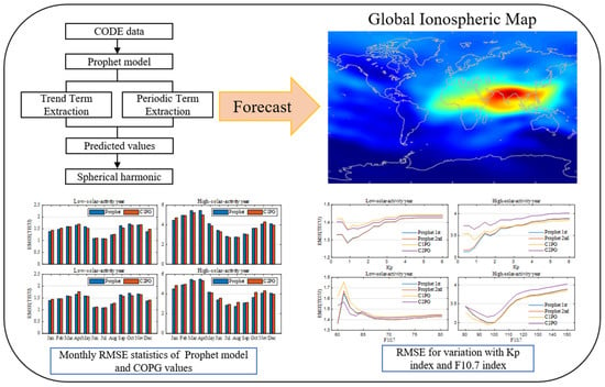
2.1. Prophet Model

The Prophet model [42] is a novel time series forecasting model based on machine learning. The advantages of the Prophet model are automatic processing of missing data, a fast-processing speed, simple parameter adjustment and complete automation. Focusing on the characteristics of the sequence of annual changes in ionospheric TEC, weekday changes and sudden changes affected by geomagnetic disturbances, the Prophet model can automatically extract and separate periodic terms and identify sudden changes and exhibits good adaptability for forecasting such time series. The Prophet model is based on the principle of decomposition followed by recombination. It decomposes the time series into four parts: trend terms, periodic terms, holiday effects, and random noise. The forecast is then combined through an additive or multiplicative model. The additive model is expressed as

$$y(t)=g(t)+s(t)+h(t)+{\epsilon }_t$$

(1)

where $t$ is the time scale; $y(t)$ is the time series, which varies with time $t$; $g(t)$ is the decomposed trend component, with no periodicity; $s(t)$ is the periodic component; $h(t)$ is the holiday effect or sudden change factor; and ${\epsilon }_t$ is random noise that obeys a normal distribution.

2.1.1. Trend Term Extraction

The Prophet model provides two methods for extracting the trend terms for different time series; a piecewise linear model and a logistic regression model. The piecewise linear model is suitable for time series without saturated growth, and its calculation formula is

$$g(t)=[k+{\mathit{\alpha }}^{\mathrm{T}}(t)\mathit{\delta }]t+[b-{\mathit{\alpha }}^{\mathrm{T}}(t){\mathit{\delta }}_j{T}_j]$$

(2)

where $k$ is the initial growth rate; ${\mathit{\alpha }}^{\mathrm{T}}(t)\mathit{\delta }$ is the slope correction value; b is the initial offset rate, and ${\mathit{\alpha }}^{\mathrm{T}}(t){\mathit{\delta }}_j{T}_j$ is the offset correction value. The logistic regression model is suitable for nonlinear time series with saturated growth, and its calculation formula is

$$g(t)=\frac{c(t)}{1+\exp (-k)(t-b)}$$

(3)

where $c$ is the saturated growth value and $k$ and $b$ are the initial growth rate and initial migration rate, respectively. As the time $t$ increases, $g$ approaches the natural saturated state $c$.

2.1.2. Periodic Term Extraction

The ionospheric TEC sequence exhibits obvious periodic characteristics. The Prophet model uses discrete Fourier series to model and extract the periodic terms of the time sequence. The calculation formula is

$$s(t)={\displaystyle \sum _{n=-N}^N{c}_n\exp \left[\frac{i2\pi nt}{P}\right]}$$

(4)

where $c_n$ are the coefficient parameters to be estimated, which satisfy $c_n~N(0,{\sigma }_c^2)$; $P$ is the time series period; and $N$ is the number of approximate terms used to fit the period. For weekday changes in the ionospheric TEC sequence, the annual periodicity $P$ is generally set to 365.25, and $N$ is set to 10. For the weekly periodicity, $P$ is set to 7, and $N$ is set to 3. With the notation

$$x(t)=\left[\exp \left(\frac{i2\pi (-N)t}{P}\right),\cdots ,\exp \left(\frac{i2\pi Nt}{P}\right)\right]$$

(5)

$s(t)$ can be expressed as the dot product of $x(t)$ with $\mathit{\beta }$, a parameter vector; and the calculation formula is

$$s(t)=x(t)\mathit{\beta }$$

(6)

where $\mathit{\beta }$ is a periodic smoothing parameter that has a regularization effect and follows a normal distribution, $\mathit{\beta }~N(0,{\sigma }^2)$. The parameter $\sigma$ can be increased or decreased to adjust the influence of the periodicity on the forecasting effect; specifically, its value is positively correlated with the influence of the periodicity on the time series.

2.2. Spherical Harmonic Function Model

Schaer first proposed using a spherical harmonic function model to fit GIMs in 1999 [43]. With the development of GNSS technology, the number of Earth observation satellites has increased. At present, CODE provides data based on more than 200 Global Navigation Satellite System (GNSS) observation stations around the world. The data are fit using 15th-order spherical harmonic functions to obtain and publish GIMs. The calculation formula for the spherical harmonic functions is

$$\mathrm{VTEC}(\beta ,\lambda )={\displaystyle \sum _{n=0}^{n_{\max }}{\displaystyle \sum _{m=0}^n\left\{{\tilde{P}}_{nm}(\sin \beta )\times ({\tilde{L}}_{A_{nm}}\cos (m\lambda )+{\tilde{L}}_{B_{nm}}\sin (m\lambda ))\right\}}}$$

(7)

where $m$ and $n$ represent the order and degree of the spherical harmonic function. ${\tilde{L}}_{A_{nm}}$ and ${\tilde{L}}_{B_{nm}}$ represent the coefficients of the associated Legendre function ${\tilde{P}}_{nm}$ in the spherical harmonic function; and $\beta$ and $\lambda$ are the latitude and longitude, respectively, of the puncture point in the geocentric solar geomagnetic coordinate system. CODE provides 15th-order historical data for 256 spherical harmonic function coefficients.

3. Data and Results

3.1. Data Source and Parameter Setting

For forecast analysis using the spherical harmonic function coefficient products released by CODE, we select 2019 as a year with lower solar activity (63.4 < F10.7 < 81.8) and 2015 as a year with higher solar activity (79.5 < F10.7 < 255.0). We select training samples with different time scales and perform sliding prediction of the spherical harmonic function coefficients for 2 specific days. Thus, we generate a global ionospheric TEC map with a resolution of 2.5° × 5°. We compare the results with C1PG and CODE’S 2-Day Predicted GIM (C2PG) to verify the accuracy and reliability of the model presented in this paper.

According to the temporal and spatial changes in the ionosphere and the characteristics of the Prophet model, the short-term forecasting of the ionospheric TEC is mainly concerned with daily periodic changes, and the trend term can be described by a model with piecewise linear growth. Therefore, we set the growth term parameter to ‘linear’, the daily periodicity parameter to ‘true’, and the seasonality parameter to ‘additive’. The actual parameter settings are shown in

Table 1. Prophet model parameter settings.

Parameter	Description	Setting	Description
growth	growth model	linear	linear growth model
daily_seasonality	daily periodicity	true	set the daily cycle
seasonality_mode	periodic term model	additive	additive model
seasonality_prior_scale	periodic scale	10.0	cyclical impact factor

after several rounds of search. For mutation point screening, the automatic screening mode of the Prophet model is adopted. For hyperparameters that characterize the flexibility scale that ‘changepoint_prior_scale’, we use the grid search method [44]. According to the extrapolation results of parameter tuning, the parameter search range is set to 0.1~0.9, and the search step is set to 0.1.

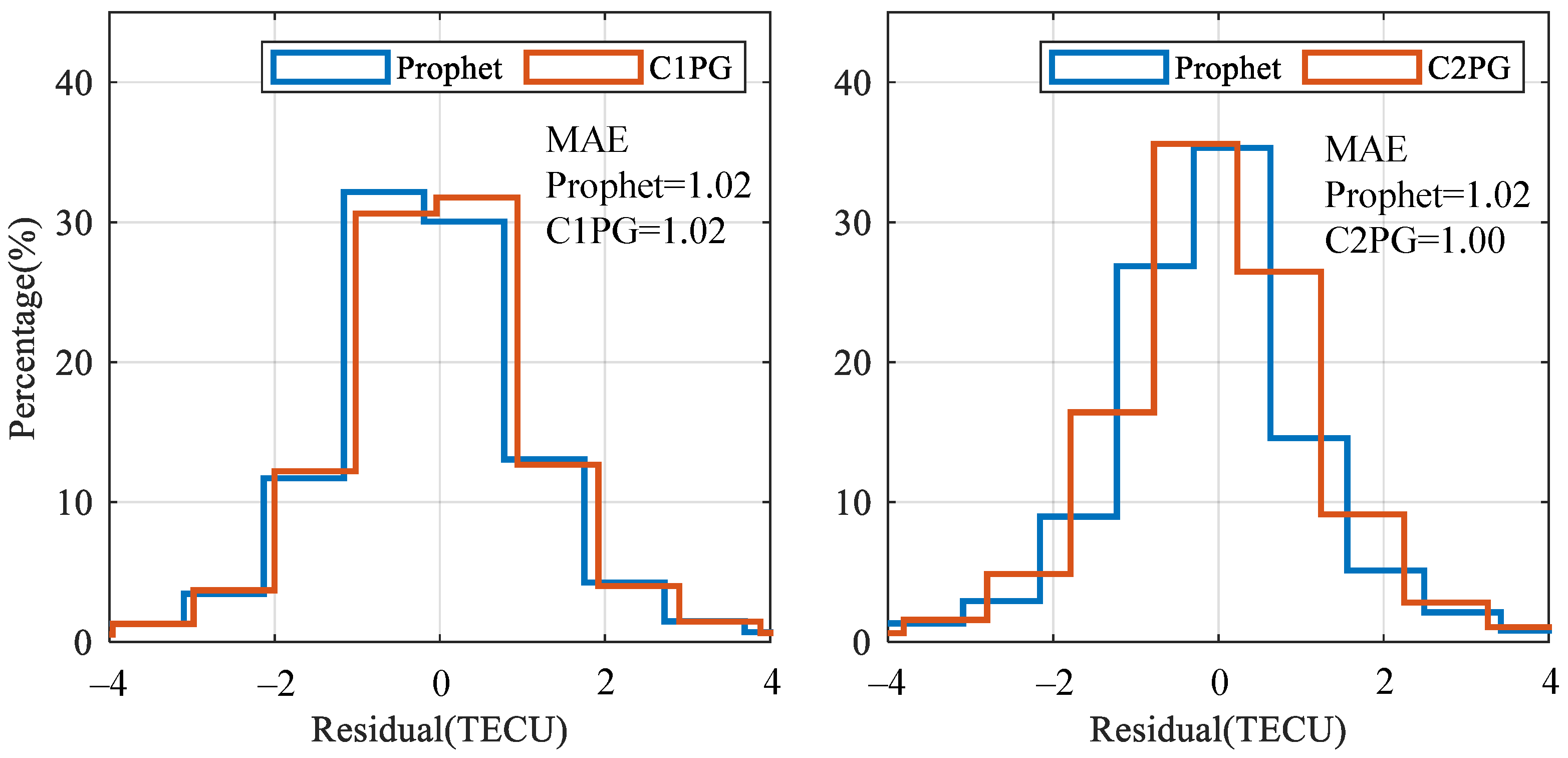
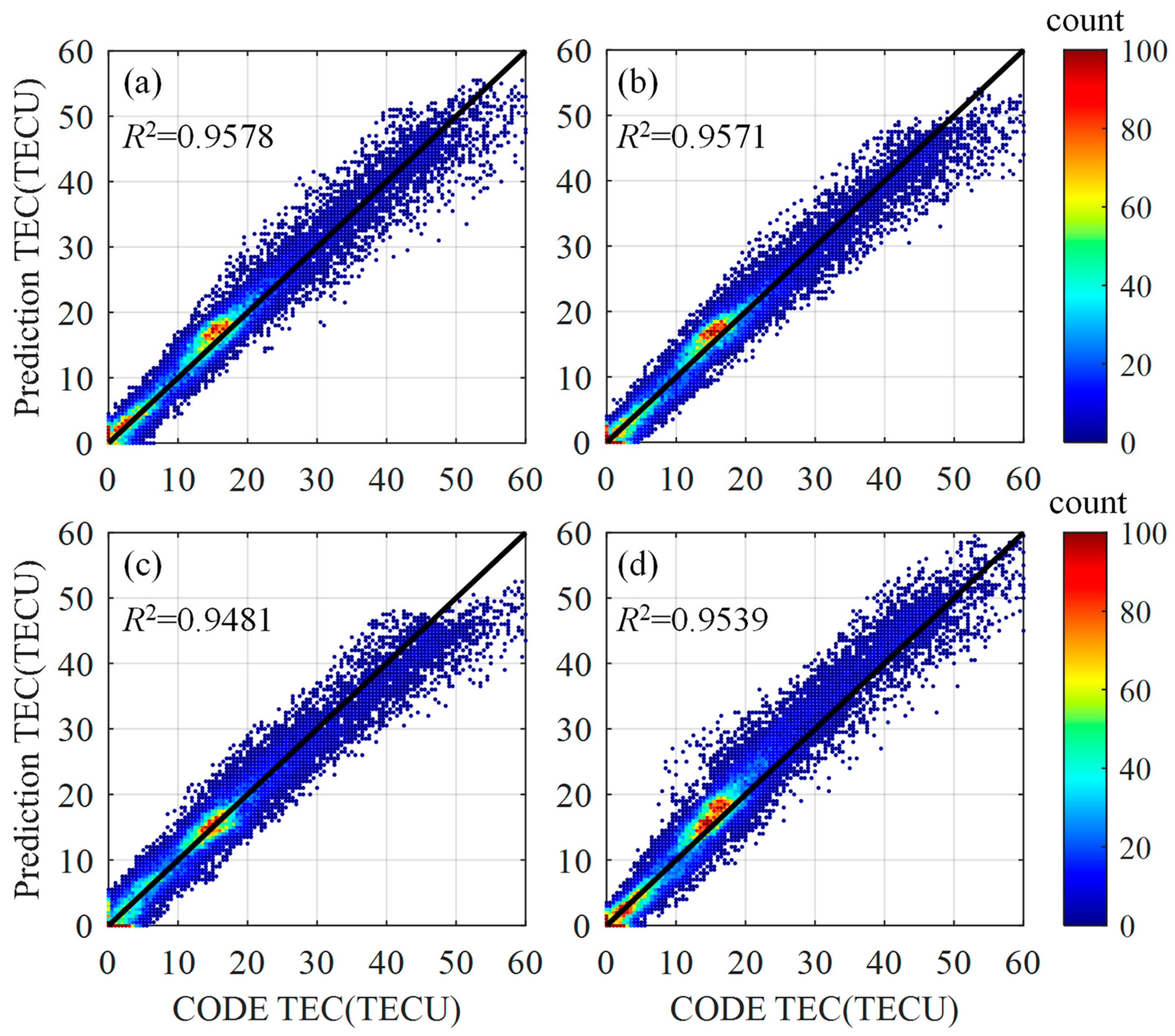
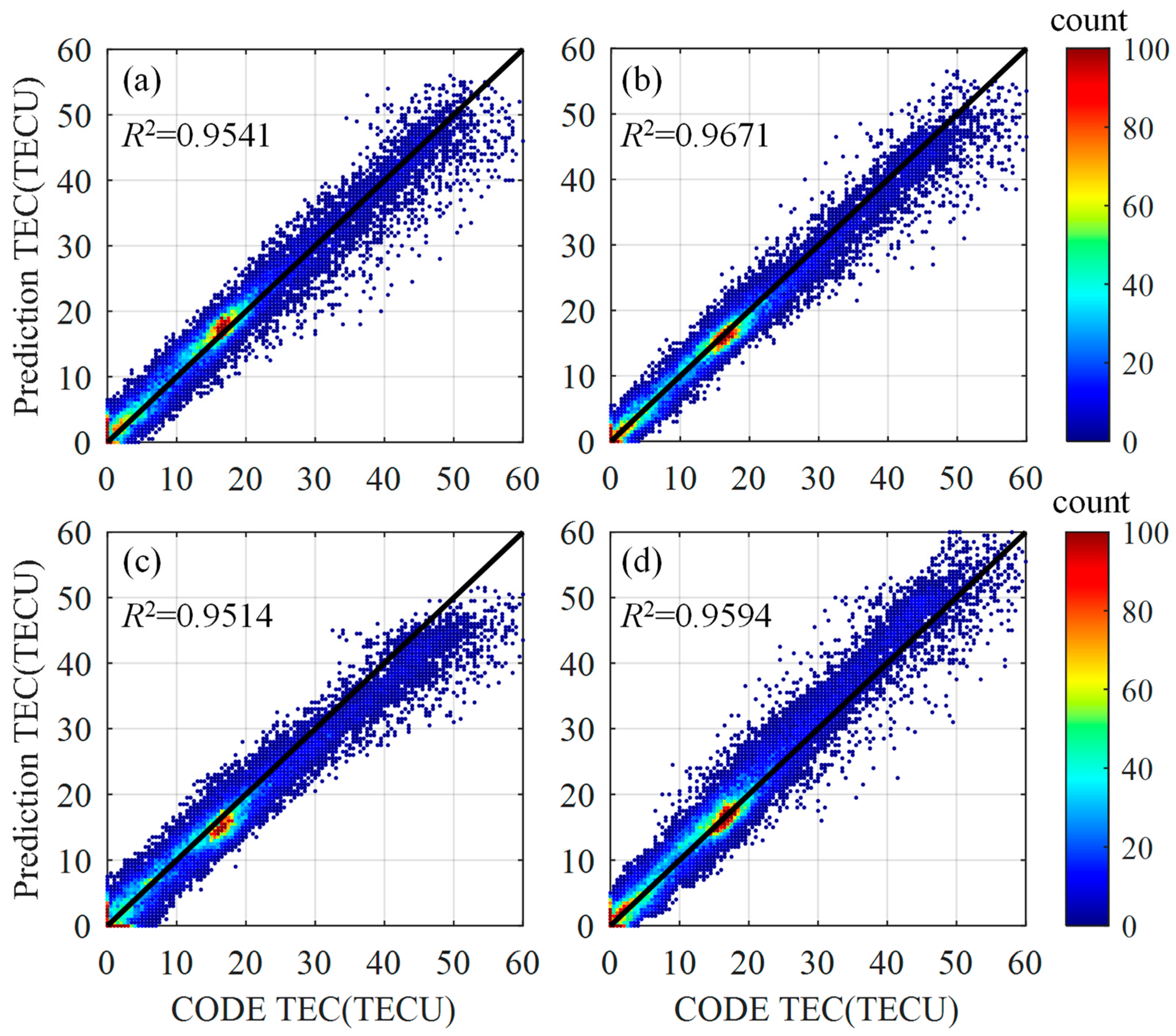
3.2. Accuracy Evaluation

To evaluate the forecasting results, we calculate the root mean square error (RMSE), mean absolute error (MAE) and correlation coefficient (R) of the model forecasted values and CODG values to analyze the forecasting effect. These metrics are calculated as

$$\mathrm{RMSE}=\sqrt{\frac{1}{n}{\displaystyle \sum _{i=1}^n{({\overline{y}}_i-y_i)}^2}}$$

(8)

$$\mathrm{MAE}=\frac{1}{n}{\displaystyle \sum _{i=1}^n\left|{\overline{y}}_i-y_i\right|}$$

(9)

$$R=\frac{\mathrm{cov}({\overline{y}}_i,y_i)}{{\sigma }_{{\overline{y}}_i}\cdot {\sigma }_{y_i}}$$

(10)

where ${\overline{y}}_i$ represents the TEC forecasted value, $y_i$ represents the CODG value, and $n$ represents the data length.

The full-year data of 2015 and 2019 were selected for the experiments to validate the model reliability. We designed 3 sets of experiments to find the optimal time-scale training set. The spherical harmonic function coefficients with time scales of 7, 15 and 30 days were used as training sets. For comparison with CODG, the 2-day data after the training set was used as the test set. The specific experimental steps are as follows:

• The 0th order spherical harmonic function coefficients were entered into the model. The last day of data from the test set was used as the validation set to determine the hyperparameter ‘changepoint_prior_scale’.
• Using the hyperparameters determined in the first step to predict 256 spherical harmonic function coefficients, the 2-day spherical forecast values were obtained.
• The predicted values were substituted into Equation (8) to calculate the GIM. We can interpolate TEC values at any latitude and longitude on demand to develop a higher-resolution ionospheric forecast product.

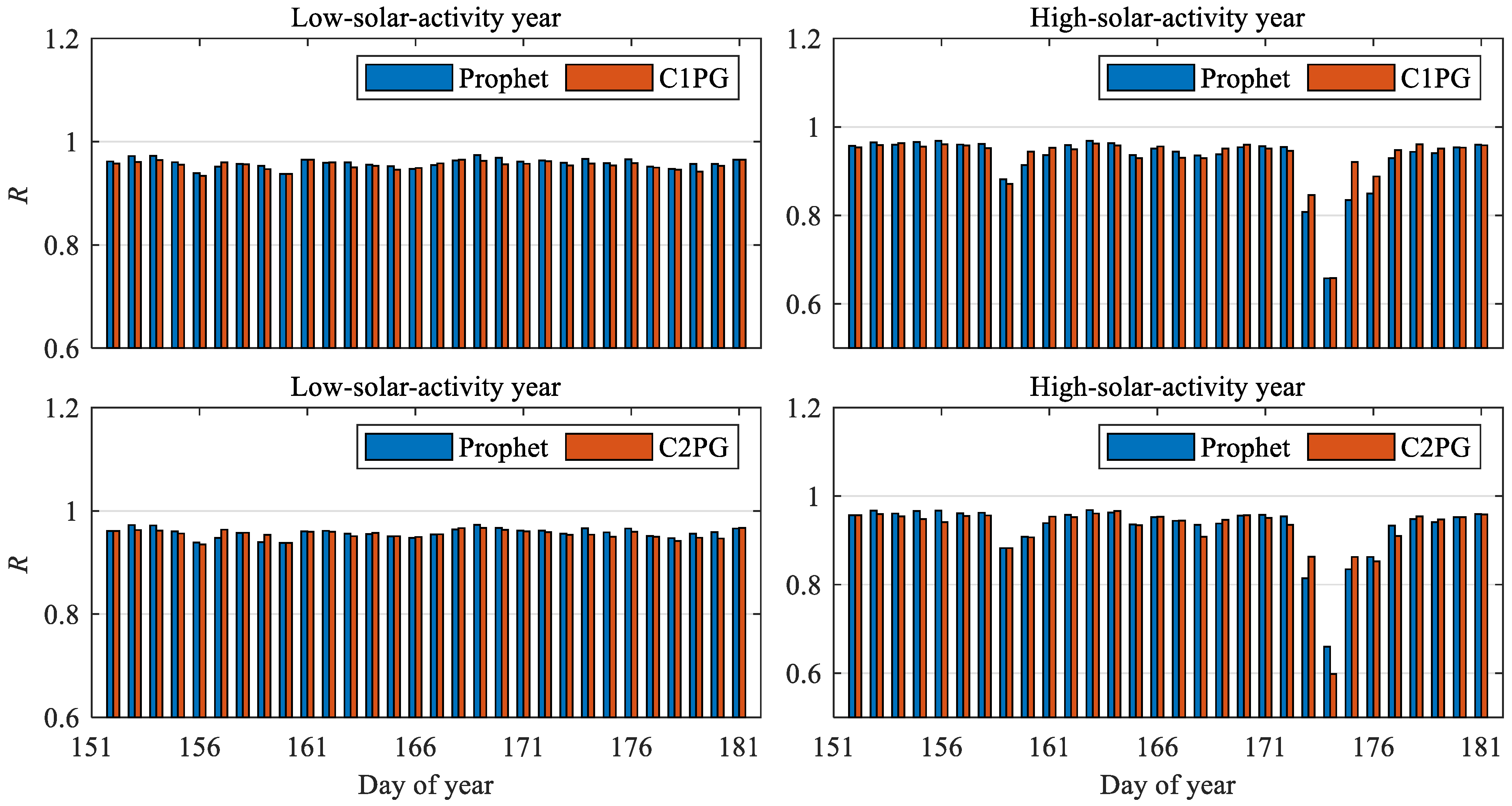
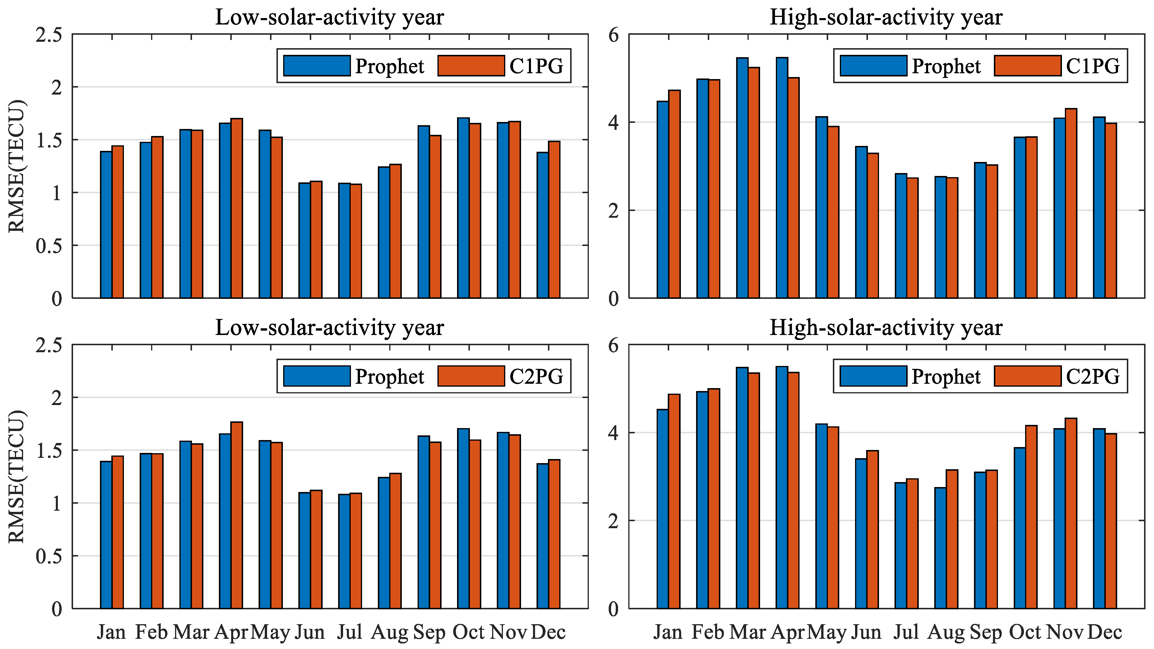
3.3. Model Performance under Low Solar Activity

We select the spherical harmonic function products released by CODE for 2019 for predictive analysis, using training data for sliding predictions to generate GIMs. At the same time, the COPG values are used to analyze the prediction accuracy of the model presented in this paper. Figure 1a,b show the 1 June forecast obtained by the Prophet model with 15 days of the training data and the corresponding COPG values, respectively. The horizontal axis is the longitude, the vertical axis is the latitude, and the time interval is 6 h. With this interval, forecasting results are produced 4 times a day. If the TEC forecasted values in some areas are negative, then we set these values to 0.

Figure 2a shows the differences between the values predicted by the Prophet model and the CODG values. Similarly, Figure 2b shows the differences between the values of the COPG values and the CODG values. The prediction residuals of the Prophet model are mostly within ±2 TECU. Regions with large errors mainly occur near the equator, which can be attributed to ionospheric equatorial anomalies. Compared with the Prophet model results, the regions with large residual errors predicted by the COPG model are significantly larger.

Table 2. Residual percentage analysis of the Prophet model and the COPG model.

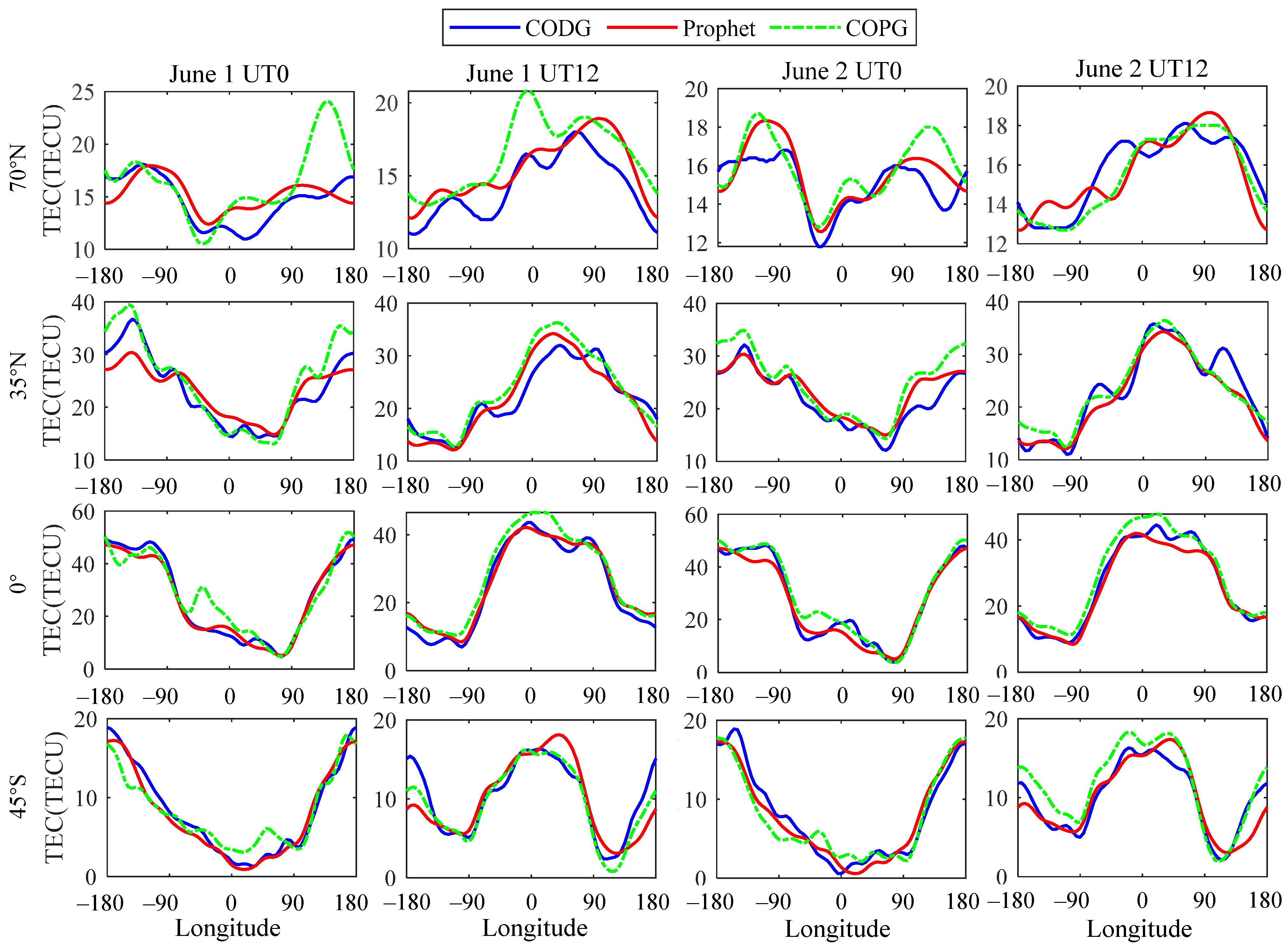
Data	Model	|Δ| < 1 TECU	|Δ| < 2 TECU	|Δ| < 3 TECU
1 June	Prophet	76.09%	92.20%	96.61%
	COPG	71.92%	89.80%	95.44%
2 June	Prophet	74.13%	93.11%	97.75%
	COPG	73.29%	92.48%	97.33%

shows the residual ratios between the forecast and CODG values for 5183 grid points at 24 time points on 1 June and 2 June. For more than 90% of the Prophet model prediction results on the second day, the absolute value of the residual error is within 2 TECU, and this absolute error is less than 3 TECU for more than 97% of the results. In contrast, the residual errors of the COPG model predictions are larger, with only approximately 70% of the residual errors being less than 1 TECU and the proportions of errors smaller than 2 TECU and 3 TECU also being lower than those of the Prophet model.

Figure 3 and Figure 4 show the correlation analysis between the global ionospheric TEC forecasted value and the CODG values on 1 and 2 June, respectively. The horizontal axis represents the CODG value, and the vertical axis represents the forecasted value. The grid points are divided with a step size of 0.3 TECU, the number of points within a 0.2 TECU radius of each grid point is counted, and this number is represented by the corresponding color. Figure 3a–c show the scatter density diagrams of the correlations between the Prophet model forecasted value and the CODG values at training time scales of 7, 15 and 30 days, respectively. Figure 3d shows the scatter density diagram of the correlation between the COPG and CODG values. It can be seen from Figure 3 that the forecasted values and the CODG values are mostly concentrated in the range of 0~10 TECU, and all four forecasting methods yield reasonably accurate forecasting results in this range. However, the distribution of the COPG values vs. the CODG values is the most disperse, and the COPG value is generally larger than the CODG value, indicating that the forecasting effect is poor. When the Prophet model takes 7 days, 15 days and 30 days of training data, the $R^2$ values between the predicted values and the CODG values are 0.9592, 0.9618 and 0.9541, respectively. These findings indicate that 15 days is the best time scale of the training data for forecasting. It can also be seen from the figure that the correlation between the forecasted values and the CODG values in Figure 3b is the best, as the distribution in Figure 3a is relatively dispersed, with the forecasted value being generally greater than the CODG value, while the forecasted values in Figure 3c are all less than 25 TECU, indicating that this model does not have a good effect in predicting the maximum value. Figure 4 shows that the correlation between the forecast and CODG values on 2 June is similar to that on 1 June. In summary, the forecasted values obtained by using 15-day historical data as the training set are the most consistent with the CODG values, indicating that the forecasting effect is the best.

Figure 5 shows statistical histograms of the forecasted residual distributions between the values predicted by the Prophet model and the COPG values in this low-solar-activity year. As seen from the figure, the forecasted residuals for the 2 investigated days are mostly within 2 TECU and forecasted values with residuals greater than 2 TECU account for only a small proportion. The forecasting results of the Prophet model on 1st day and 2nd day have MAEs of 1.02 TECU and 1.02 TECU, respectively, whereas the MAEs of the COPG model are 1.02 TECU and 1.00 TECU, respectively. These findings show that both models have similar accuracy.

To analyze the prediction effects at different latitudes and longitudes, we plot the variations in the CODG value, the Prophet forecasted value and the COPG value with latitude in Figure 6. As seen from this figure, the Prophet forecasted value is closer to the CODG value in most regions, indicating that the Prophet model can accurately predict the TEC trend, and both the maximum and minimum values are consistent with the real values. In contrast, the prediction effect of the COPG model at the maximum value is not accurate, and this deficiency is more obvious in the high-latitude areas of the Northern and Southern Hemispheres.

3.4. Model Performance under High Solar Activity

To further verify the reliability of the model, 2015 is selected as a year with high solar activity for forecast analysis. The global ionospheric TEC maps on 1 June to 31 June are again predicted with 7 days, 15 days and 30 days of training data to assess the forecasting accuracy and reliability. Figure 7 compares the forecasting results of the Prophet model with the COPG and CODG values on 1 June 2015. It can be seen that the maximum annual TEC in this year of high solar activity is 65 TECU. The Prophet model has a basically accurate prediction effect, with the maximum predicted value being approximately 5 TECU smaller. The global distribution is close to that of the CODG values.

Figure 8 and Figure 9 show the correlation analysis between the global ionospheric TEC forecasted value and the CODG values on 1 June and 2 June 2015, respectively. It can be seen that the annual TEC value in a year of high solar activity is significantly larger. The horizontal axis represents the CODG value, and the vertical axis represents the model forecasted value, the same as in Figure 3. Figure 8a–d present the scatter density diagrams of the correlations between the Prophet model forecasted values at the 7-day, 15-day and 30-day training scales and COPG values, respectively, and the CODG values. We divide the grid points with a step size of 0.5 TECU and count the number of points within a radius of 0.2 TECU of each grid point. As seen in this figure, the annual TEC values in this year with high solar activity are significantly larger than those in the previous analysis, reaching a maximum of 60 TECU. The 7-day Prophet model forecasted values, COPG values and CODG values are dispersed and have weak correlations. The prediction effect of the 30-day Prophet model for the maximum TEC value is not ideal, which may be related to the long duration of the training data. In general, the 15-day Prophet model shows the best prediction effect and the highest correlation with the CODG values, with the $R^2$ values of this Prophet model for the 2 investigated days being 0.96 and 0.97.

Figure 10 shows histograms of the prediction residuals of the Prophet model and the COPG values. Due to the violent influence of solar activity, the TEC values are relatively large, leading to large forecast errors. In this figure, only 30% of the values predicted by the Prophet model on the first day are within 1 TECU; however, residual values of less than 10 TECU still account for a high proportion, with an average residual of 2.9 TECU on the first day. By comparison, values of less than 1 TECU account for a smaller proportion of the residuals of the COPG model, with an average residual of 2.8 TECU on the first day. On the second day, the average residual values of the Prophet and COPG models are 2.9 TECU and 3.0 TECU, respectively, and the residuals of the Prophet model are generally closer to 0. This shows that the Prophet model has smaller prediction residuals and higher accuracy.

Figure 11 shows the CODG value, the Prophet forecasted value and the COPG value with latitude. As seen from the figure, the 2-day forecasts from both models accurately predicted the trend of TEC changes. Compared with the two models, the Prophet model is closer to the CODG value, which is similar to low-solar-activity year. The prediction error of COPG value at the maximum value is obviously larger, which is especially obvious in high latitude areas.

Figure 12 shows the prediction results of the Prophet and COPG models under different longitude and latitude interpolations. Both models can accurately predict the TEC trend at a single point. The Prophet model is more accurate in predicting the overall trend, and the COPG model is more precise.

Table 3. Accuracy comparison of the Prophet and COPG models at different latitudes at longitude 120°E.

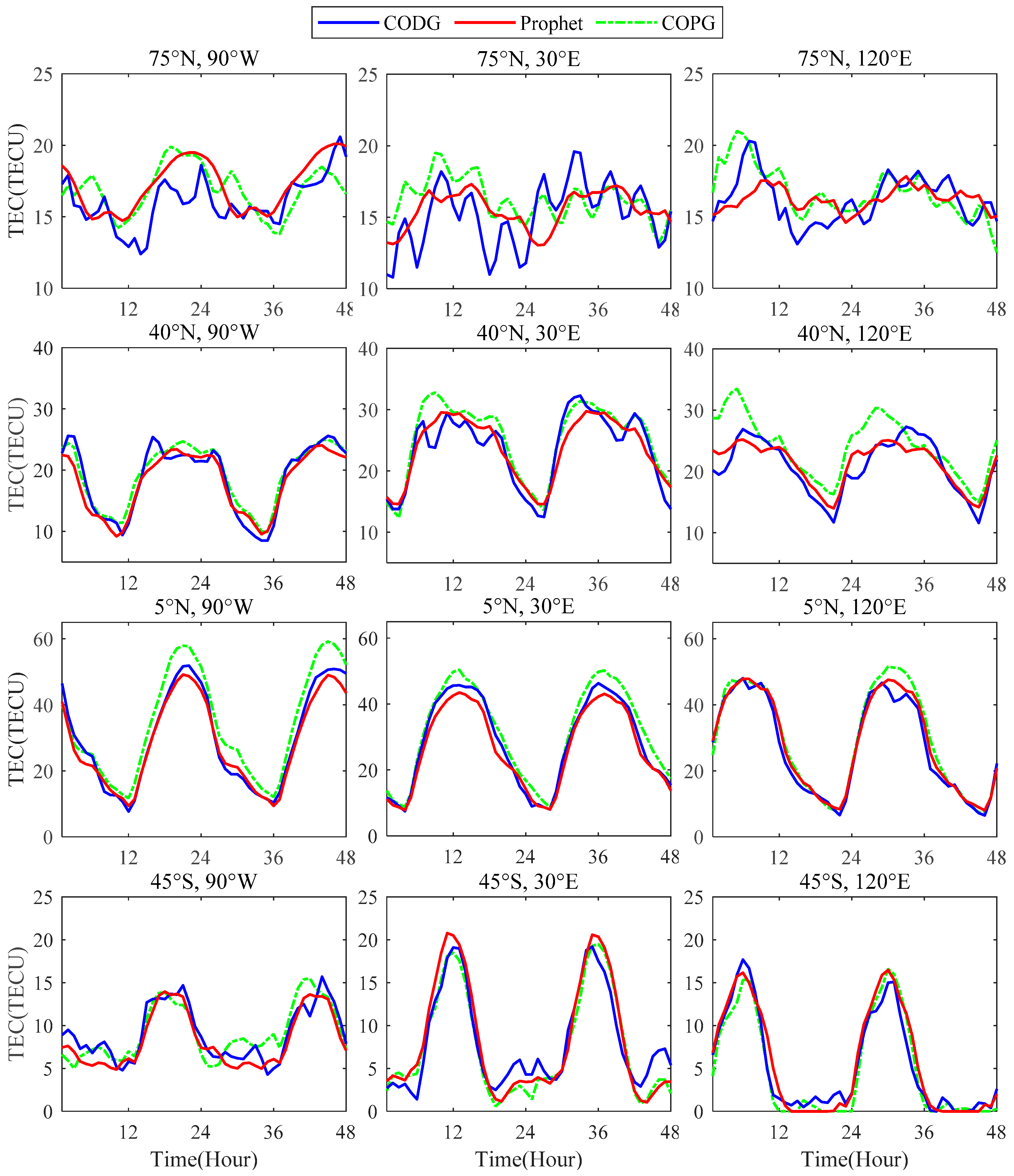
Latitude and Longitude	Forecasting Model	Performance Index
		RMSE (TECU)	MAE (TECU)	R
75°N, 120°E	Prophet	1.5	1.2	0.42
	COPG	1.6	1.2	0.63
40°N, 120°E	Prophet	2.0	1.6	0.91
	COPG	4.6	3.7	0.76
5°N, 120°E	Prophet	2.2	1.7	0.99
	COPG	3.7	2.6	0.98
45°S, 120°E	Prophet	1.4	1.1	0.97
	COPG	1.5	1.2	0.97

shows a forecast assessment for different latitudes at a longitude of 120°E. The prediction error of the Prophet model in high-latitude areas is small, but the correlation is lower than that of the COPG model. This reflects the irregular change in the TEC in low-latitude regions, for which the Prophet model is not ideally suited. Nevertheless, the prediction effect of the Prophet model is significantly better than that of the COPG model at middle and low latitudes. Compared with the COPG model, the RMSE of the Prophet model at middle and low latitudes is reduced by 2.6 TECU and 2.1 TECU, respectively, and the MAE is lower by 1.4 TECU and 0.9 TECU, respectively. It is worth noting that in the Southern Hemisphere, there are some 0 values in the prediction results of the Prophet model, and the prediction accuracy is slightly higher than that of the COPG model. On the whole, the prediction accuracy of the Prophet model is better than that of the COPG model.

Figure 13 shows the RMSE statistics of the two models in June for a low-solar-activity year and a high-solar-activity year. Compared with the results of C1PG and C2PG. The root mean square errors (RMSE) of the first day forecasts for the considered days of the low-solar-activity year and the high-solar-activity year are significantly reduced. For the low-solar-activity year, we calculated the total RMSE of 720 hourly forecasted values with CODG values for the forecast 30 days, and the RMSE of the Prophet model for the first day forecasts for the considered days and the second day forecasts for the considered days both are 1.1 TECU. For the high-solar-activity year, the Prophet model forecasts an RMSE of 3.4 TECU for both the first and second day. The forecast accuracy does not decrease with time.

Figure 14 shows the correlation coefficient statistics of the two models at the low-solar-activity year and the high-solar-activity year. In the low-solar-activity year, the correlation coefficients between the Prophet model and CODG values are all above 0.93. Comparing the correlation coefficients between the two models and the CODG values, the Prophet model forecast of 24 days outperforms the COPG values in the first day forecasts for the considered days, and the Prophet model forecast of 20 days outperforms the COPG values in the second day forecasts for the considered days. In the high-solar-activity year, comparing the correlation coefficients between the two models and the CODG values, the Prophet model forecast of 17 days outperforms the COPG values in the first day forecasts for the considered days and the Prophet model forecast of 19 days outperforms the COPG values in the second day forecasts for the considered days. The average of correlation coefficients for the predicted 30 days between the predicted results and the CODG values on the first day and second day in the low-solar-activity year both are 0.96. The average of correlation coefficients for the predicted 30 days between the predicted results and CODG values on the first day and second day in the high-solar-activity year both are 0.93. These results indicate that the predicted values are highly correlated with the actual values and that the forecasting results are reliable. The correlation between the two model predictions is poor during extremely large magnetic storm days 173 and 174.

Figure 15 shows the RMSE statistics of the two models at low-solar-activity year and high-solar-activity year. As seen from the figure, the forecasted error is low for June, July and August throughout the year. In 2015, a year of intense solar activity, the error in the Prophet model forecasts for March, influenced by magnetic storms, was slightly larger. We calculated the RMSE for both models for a full year. The RMSEs of the Prophet model for the first and second day of the low-solar-activity year are both 1.5 TECU. The RMSEs of the Prophet model for the first and second day of the high-solar-activity year both are 4.1 TECU. Therefore, the Prophet model has good performance in global forecasting during geomagnetic quiet periods, the difference in performance between the two days is not significant.

Figure 16 shows the variation of RMSE with Kp index and F10.7 index. As can be seen from the top left and top right panels, the RMSE increases with increasing Kp index. The overall performance of the Prophet model for low-solar-activity years is better than the COPG values. In the high-solar-activity year, the Prophet model performs better when Kp < 3. The Prophet forecasted error is greater than C1PG and less than C2PG when Kp > 3. Analysis based on solar activity, the RMSE of the two models is larger when the f10.7 index is less than 65 in the low-solar-activity year, and the forecast accuracy remains stable as the f10.7 index increases. The RMSE of the high-solar-activity year has a minimum value at an F10.7 index of 95 and gradually increases with the intensity of solar activity. Prophet’s two-day forecast accuracy remained stable, while C1PG and C2PG values differed considerably.

4. Discussion

Machine learning is suitable in finding patterns and relationships from historical data to solve problems. Computer systems learn by example and extract useful information from a large set of historical data in a mathematical approach. It usually contains a large amount of data, spanning as many parameters as possible [45]. In the paper, the Prophet model was used to take into account multiple factors affecting forecasting when modeling and forecasting the 15th-order spherical harmonic function coefficients of the ionosphere and generating a global ionospheric TEC map. Training samples with three-time scales of 7 days, 15 days, and 30 days were selected for experimental analysis based on the unique ionospheric activity occurring in years of quiet solar activity and high solar activity. The RMSEs, MAEs and correlation coefficients were used for evaluation.

We used the Prophet model to perform sliding prediction of the spherical harmonic coefficients for a month. The results show that the model exhibits good performance in both years with low solar activity and years with high solar activity. The average of correlation coefficients for the predicted 30 days between the predicted results and the CODG values on the first day and second day in the low-solar-activity year are both 0.96. The average of correlation coefficients for the predicted 30 days between the predicted results and CODG values on the first day and second day in the high-solar-activity year are both 0.93. These results indicate that the predicted values are highly correlated with the actual values and that the forecasting results are reliable. The prediction accuracy of this model is affected by the number of days of training data used. We calculated the correlation coefficients for three sets of experiments for the predicted days of low solar activity year and the predicted days of high solar activity year. In low solar activity years, the correlation coefficients between the CODG values and the forecasts derived from the seven days, 15 days, and 30 days’ time scales as training sets are 0.97, 0.98, and 0.97, respectively. In high solar activity years, these indicators were 0.97, 0.98 and 0.97. Specifically, the accuracy of the prediction results obtained using a 15-day training set is the best. The RMSEs for the two forecasted days of the low-solar-activity year were 1.1 TECU and 0.9 TECU, and the MAEs were 0.8 TECU and 0.6 TECU, respectively. The RMSEs for the two forecasted days in the high-solar-activity year were 2.4 TECU and 2.3 TECU, and the MAEs were 1.8 TECU and 1.6 TECU, respectively. Overall, a time scale of 15 days data is appropriate as a training set in short-term forecasting.

With the model presented in this paper, the prediction effects at middle and low latitudes were the best, and the prediction accuracy for the Northern Hemisphere was better than that for the Southern Hemisphere. The prediction error was lower than that of the COPG model, possibly due to the density of GNSS stations in the northern hemisphere, the more accurate data collected for the history, and the better quality of the training set data. The low number of GNSS receivers in the southern hemisphere led to missing ionospheric modeling details, which affects forecast accuracy. The trend of TEC changes could be accurately predicted in high-latitude areas, but the prediction of details was not precise, leading to a relatively slight correlation. This may be due to how the ionosphere is calmer at high latitudes with less TEC changes that are less cyclical, resulting in a low correlation between forecasted values and CODG values. In the future, we will analyze and discuss spherical harmonic function coefficients of various orders, incorporate geographical factors into the prediction model, and further optimize and improve the model.

5. Conclusions

We address several problems faced by traditional forecasting models, such as the consideration of relatively few factors, complex parameter settings and unstable forecasting effects. This paper proposes a global ionospheric TEC prediction model based on machine learning. The model combines indirect forecasting methods from previous studies with machine learning methods to achieve a global TEC map forecast for the next two days. The results show that the Prophet model has good accuracy for both 2-day forecasts. The machine learning model—the Prophet model—is robust and outperforms the results of C2PG when comparing with COPG in terms of their performance. In general, the model can be considered applicable and can provide a powerful data basis for GNSS error correction. This provides more stable and accurate positioning services for single-frequency GNSS users. In the future, we will consider more influencing factors and training models considering more characteristic conditions to achieve better prediction results.

References

- Komjathy, A. Global Ionospheric Total Electron Content Mapping Using the Global Positioning System. Ph.D. Thesis, University of New Brunswick Fredericton, Fredericton, NB, Canada, 1997. [Google Scholar]
- Rovira-Garcia, A.; Juan, J.M.; Sanz, J.; González-Casado, G. A worldwide ionospheric model for fast precise point positioning. IEEE Trans. Geosci. Remote Sens. 2015, 53, 4596–4604. [Google Scholar] [CrossRef] [Green Version]
- Yuan, Y.; Tscherning, C.C.; Knudsen, P.; Xu, G.; Ou, J. The ionospheric eclipse factor method (IEFM) and its application to determining the ionospheric delay for GPS. J. Geod. 2008, 82, 1–8. [Google Scholar] [CrossRef]
- Cai, X.; Burns, A.G.; Wang, W.; Qian, L.; Liu, J.; Solomon, S.C.; Eastes, R.W.; Daniell, R.E.; Martinis, C.R.; McClintock, W.E.; et al. Observation of postsunset OI 135.6 nm radiance enhancement over south America by the GOLD Mission. J. Geophys. Res. Space Phys. 2021, 126, e2020JA028108. [Google Scholar] [CrossRef]
- Martinis, C.; Daniell, R.; Eastes, R.; Norrell, J.; Smith, J.; Klenzing, J.; Solomon, S.; Burns, A. Longitudinal variation of postsunset plasma depletions from the global-scale observations of the limb and disk (GOLD) mission. J. Geophys. Res. Space Phys. 2021, 126, e2020JA028510. [Google Scholar] [CrossRef]
- Li, Q.; Hao, Y.; Zhang, D.; Xiao, Z. Nighttime enhancements in the midlatitude ionosphere and their relation to the plasmasphere. J. Geophys. Res. Space Phys. 2018, 123, 7686–7696. [Google Scholar] [CrossRef]
- Klimenko, M.; Zakharenkova, I.E.; Klimenko, V.V.; Lukianova, R.Y.; Cherniak, I. Simulation and observations of the polar tongue of ionization at different heights during the 2015 St. Patrick’s day storms. Space Weather 2019, 17, 1073–1089. [Google Scholar] [CrossRef] [Green Version]
- Jin, S.; Jin, R.; Li, D. GPS detection of ionospheric rayleigh wave and its source following the 2012 Haida Gwaii earthquake. J. Geophys. Res. Space Phys. 2017, 122, 1360–1372. [Google Scholar] [CrossRef]
- Jin, S. Two-mode ionospheric disturbances following the 2005 Northern California offshore earthquake from GPS measurements. J. Geophys. Res. Space Phys. 2018, 123, 8587–8598. [Google Scholar] [CrossRef]
- Liu, T.; Zhang, B.; Yuan, Y.; Li, M. Real-time precise point positioning (RTPPP) with raw observations and its application in real-time regional ionospheric VTEC modeling. J. Geod. 2018, 92, 1267–1283. [Google Scholar] [CrossRef]
- Wang, Y.; Yao, Y.; Zhang, L.; Fang, M. A refinement method of real-time ionospheric model for China. Remote Sens. 2020, 12, 3354. [Google Scholar] [CrossRef]
- Jin, S.; Gao, C.; Yuan, L.; Guo, P.; Calabia, A.; Ruan, H.; Luo, P. Long-term variations of plasmaspheric total electron content from topside GPS observations on LEO satellites. Remote Sens. 2021, 13, 545. [Google Scholar] [CrossRef]
- Zhang, W.; Huo, X.; Yuan, Y.; Li, Z.; Wang, N. Algorithm research using GNSS-TEC data to calibrate TEC calculated by the IRI-2016 model over China. Remote Sens. 2021, 13, 4002. [Google Scholar] [CrossRef]
- He, X.; Bos, M.S.; Montillet, J.P.; Fernandes, R.; Melbourne, T.; Jiang, W.; Li, W. Spatial variations of stochastic noise properties in GPS time series. Remote Sens. 2021, 13, 4534. [Google Scholar] [CrossRef]
- Klobuchar, J.A. Ionospheric time-delay algorithms for single-frequency GPS users. IEEE Trans. Aerosp. Electron. Syst. 1987, AES-23, 325–331. [Google Scholar] [CrossRef]
- Yuan, Y.; Huo, X.; Ou, J.; Zhang, K.; Chai, Y.; Wen, D.; Grenfell, R. Refining the Klobuchar ionospheric coefficients based on GPS observations. IEEE Trans. Aerosp. Electron. Syst. 2008, 44, 1498–1510. [Google Scholar] [CrossRef]
- Pongracic, B.; Wu, F.; Fathollahi, L.; Brčić, D. Midlatitude Klobuchar correction model based on the K-means clustering of ionospheric daily variations. GPS Solut. 2019, 23, 80. [Google Scholar] [CrossRef]
- Nava, B.; Coïsson, P.; Radicella, S.M. A new version of the NeQuick ionosphere electron density model. J. Atmos. Sol.-Terr. Phy. 2008, 70, 1856–1862. [Google Scholar] [CrossRef]
- Yuan, Y.; Wang, N.; Li, Z.; Huo, X. The BeiDou global broadcast ionospheric delay correction model (BDGIM) and its preliminary performance evaluation results. Navigation 2019, 66, 55–69. [Google Scholar] [CrossRef] [Green Version]
- Bilitza, D.; McKinnell, L.A.; Reinisch, B.; Rowell, T.F. The international reference ionosphere today and in the future. J. Geod. 2011, 85, 909–920. [Google Scholar] [CrossRef]
- Yuan, Y.; Ou, J. An improvement to ionospheric delay correction for single-frequency GPS users—The APR-I scheme. J. Geod. 2001, 75, 331–336. [Google Scholar] [CrossRef]
- Yuan, Y.; Ou, J. Differential Areas for Differential Stations (DADS): A new method of establishing grid ionospheric model. Chin. Sci. Bull. 2002, 47, 1033–1036. [Google Scholar] [CrossRef]
- Bilitza, D.; Altadill, D.; Truhlik, V.; Shubin, V.; Galkin, I.; Reinisch, B.; Huang, X. International reference ionosphere 2016: From ionospheric climate to real-time weather predictions. Space Weather 2017, 15, 418–429. [Google Scholar] [CrossRef]
- Feltens, J. The international GPS service (IGS) ionosphere working group. Adv. Space Res. 2003, 31, 635–644. [Google Scholar] [CrossRef]
- Hernández-Pajares, M.; Juan, J.M.; Sanz, J.; Orus, R.; Garcia-Rigo, A.; Feltens, J.; Komjathy, A.; Schaer, S.C.; Krankowski, A. The IGS VTEC Maps: A reliable source of ionospheric information since 1998. J. Geod. 2009, 83, 263–275. [Google Scholar] [CrossRef]
- Dow, J.M.; Neilan, R.E.; Rizos, C. The international GNSS service in a changing landscape of global navigation satellite systems. J. Geod. 2009, 83, 191–198. [Google Scholar] [CrossRef]
- Jee, G.; Lee, H.B.; Kim, Y.H.; Chung, J.K.; Cho, J. Assessment of GPS global ionosphere maps (GIM) by comparison between CODE GIM and TOPEX/Jason TEC data: Ionospheric perspective. J. Geophys. Res. Space Phys. 2010, 115, A10319. [Google Scholar] [CrossRef] [Green Version]
- Roma-Dollase, D.; Hernández-Pajares, M.; Krankowski, A.; Kotulak, K.; Ghoddousi-Fard, R.; Yuan, Y.; Li, Z.; Zhang, H.; Shi, C.; Wang, C. Consistency of seven different GNSS global ionospheric mapping techniques during one solar cycle. J. Geod. 2018, 92, 691–706. [Google Scholar] [CrossRef] [Green Version]
- Tulunay, E.; Senalp, E.T.; Radicella, S.M.; Tulunay, Y. Forecasting total electron content maps by neural network technique. Radio Sci. 2006, 41, RS4016. [Google Scholar] [CrossRef]
- Xia, G.; Liu, Y.; Wei, T.; Wang, Z.; Huang, W.; Du, Z.; Zhang, Z.; Wang, X.; Zhou, C. Ionospheric TEC forecast model based on Ssupport vector machine with GPU acceleration in the China region. Adv. Space Res. 2021, 68, 1377–1389. [Google Scholar] [CrossRef]
- Zhukov, A.V.; Sidorov, D.; Mylnikova, A.; Yasyukevich, Y. Machine learning methodology for ionosphere total electron content nowcasting. Int. J. Artif. Intell. 2018, 16, 144–157. [Google Scholar] [CrossRef]
- Zhukov, A.V.; Yasyukevich, Y.V.; Bykov, A.E. GIMLi: Global ionospheric total electron content model based on machine learning. GPS Solut. 2021, 25, 19. [Google Scholar] [CrossRef]
- Huang, Z.; Yuan, H. Ionospheric single-station TEC short-term forecast using RBF neural network. Radio Sci. 2014, 49, 283–292. [Google Scholar] [CrossRef]
- Lee, S.; Ji, E.Y.; Moon, Y.J.; Park, E. One-day forecasting of global TEC using a novel deep learning model. Space Weather 2021, 19, e2020SW002600. [Google Scholar] [CrossRef]
- Srivani, I.; Prasad, G.S.V.; Ratnam, D.V. A Deep Learning-based approach to forecast ionospheric delays for GPS signals. IEEE Geosci. Remote Sens. Lett. 2019, 16, 1180–1184. [Google Scholar] [CrossRef]
- Ruwali, A.; Kumar, A.S.; Prakash, K.B.; Sivavaraprasad, G.; Ratnam, D.V. Implementation of hybrid deep learning model (LSTM-CNN) for ionospheric TEC forecasting using GPS data. IEEE Geosci. Remote Sens. Lett. 2020, 18, 1004–1008. [Google Scholar] [CrossRef]
- Li, Z.; Cheng, Z.; Feng, C.; Li, W.; Li, H. A study of prediction models for ionosphere. Chin. J. Geophys. 2007, 50, 307–319. [Google Scholar] [CrossRef]
- Wang, C.; Xin, S.; Liu, X.; Shi, C.; Fan, L. Prediction of global ionospheric VTEC maps using an adaptive autoregressive model. Earth Planets Space 2018, 70, 1–14. [Google Scholar] [CrossRef] [Green Version]
- Wang, X.; Bian, S.; Li, Z.; Ke, J.; Ren, Q.; Pan, X. Prediction of global ionospheric TEC using the semiparametric kernel estimation method. Chin. J. Geophys. 2020, 63, 1271–1281. [Google Scholar] [CrossRef]
- Qiu, F.; Pan, X.; Luo, X.; Lai, Z.; Jiang, K.; Wang, G. Global ionospheric TEC prediction model integrated with semiparametric kernel estimation and autoregressive compensation. Chin. J. Geophys. 2021, 64, 3021–3029. [Google Scholar] [CrossRef]
- Liu, L.; Zou, S.; Yao, Y.; Wang, Z. Forecasting global ionospheric TEC using deep learning approach. Space Weather 2020, 18, e2020SW002501. [Google Scholar] [CrossRef]
- Taylor, S.J.; Letham, B. Forecasting at scale. Am. Stat. 2018, 72, 37–45. [Google Scholar] [CrossRef]
- Schaer, S. Mapping and Predicting the Earth’s Ionosphere Using the Global Positioning System. Ph.D. Thesis, University of Bern, Bern, Switzerland, 1999. [Google Scholar]
- Tian, R.; Dong, X. Ionosphere VTEC prediction model fused with wavelet decomposition and Prophet framework. Syst. Eng. Electron. 2021, 43, 610–622. [Google Scholar] [CrossRef]
- Zewdie, G.K.; Valladares, K.; Cohen, M.B.; Lary, D.J.; Ramani, D.; Tsidu, G.M. Data-driven forecasting of low-latitude ionospheric total electron content using the random forest and LSTM machine learning methods. Space Weather 2021, 19, e2020SW002639. [Google Scholar] [CrossRef]