LSNet: Learned Sampling Network for 3D Object Detection from Point Clouds

Abstract

The3D object detection of LiDAR point cloud data has generated widespread discussion and implementation in recent years. In this paper, we concentrate on exploring the sampling method of point-based 3D object detection in autonomous driving scenarios, a process which attempts to reduce expenditure by reaching sufficient accuracy using fewer selected points. FPS (farthest point sampling), the most used sampling method, works poorly in small sampling size cases, and, limited by the massive points, some newly proposed sampling methods using deep learning are not suitable for autonomous driving scenarios. To address these issues, we propose the learned sampling network (LSNet), a single-stage 3D object detection network containing an LS module that can sample important points through deep learning. This advanced approach can sample points with a task-specific focus while also being differentiable. Additionally, the LS module is streamlined for computational efficiency and transferability to replace more primitive sampling methods in other point-based networks. To reduce the issue of the high repetition rates of sampled points, a sampling loss algorithm was developed. The LS module was validated with the KITTI dataset and outperformed the other sampling methods, such as FPS and F-FPS (FPS based on feature distance). Finally, LSNet achieves acceptable accuracy with only 128 sampled points and shows promising results when the number of sampled points is small, yielding up to a 60% improvement against competing methods with eight sampled points.

1. Introduction

Three-dimensional data captured by LiDAR and the RGB-D camera have applications in various fields such as autonomous driving, virtual reality, and robotics. Many deep learning techniques have been applied to point cloud tasks such as point cloud classification, segmentation, completion, and generation. In this paper, we focus on 3D object detection of autonomous driving.

In recent years, 3D object detection of autonomous driving has been a major focus. Refs. [1,2,3,4] fuse point clouds and images together to detect 3D objects. In this paper, we focus on the processing of point clouds. With a point cloud captured by LiDAR, the different methodologies to approach this issue can be classified as view-based, point-based, and voxel-based methods. Additionally, some methods utilize the advantages of both the point-based method and voxel-based method to enable both high-quality 3D proposal generation and flexible receptive fields to improve 3D detection performance. With the massive number of raw points in a point cloud, it is not trivial to downsample the point cloud data efficiently and reserve as many meaningful points as possible. With this said, the sampling approaches themselves have received comparatively less attention.

View-based methods project the 3D point cloud data into different 2D views so that mature 2D convolution techniques can be applied to solve the problem efficiently. The downsampling process is reflected in both the pooling process and the step size of convolution. Voxel-based methods view the 3D point cloud space as a cube and divide it into voxels. This means the size of the sampled point subset can be controlled by the length, width, and height of each voxel, while the step size of 3D convolution and 3D pooling can also downsample the data. Additionally, point-based methods take the raw point cloud as input and generate predictions based on each point. This causes the point-based methods to suffer from a heavy computational burden due to the need to process so much data. Ref. [5] addressed this issue and proposed an efficient and lightweight neural architecture for semantic segmentation task of large-scale point clouds. Ref. [6] introduced kernel point convolution to improve the efficiency of feature extraction in point-based methods. Hence, developing an appropriate sampling strategy has become a crucial issue.

In a point-based model, one naive approach is to sample points randomly. The most widely used method is furthest-point-sampling (FPS), which selects a group of points that are farthest apart from each other based on their 3D Euclidean distance. However, there is one sampling approach that first voxelizes the whole 3D space and only preserves one point in each voxel. KPConv [6] used grid subsampling and chose barycenters of the original input points contained in all non-empty grid cells. The 3DSSD [7] utilizes the F-FPS and FS methods. F-FPS samples points based on feature distance instead of Euclidean distance in FPS, while FS is the fusion of D-FPS(FPS) and F-FPS. Crucially, these sampling strategies are non-learned approaches and cannot preserve important points when the sampling size is small, leading to poor performance. Recently there have been a few learned approaches. Refs. [8,9,10] proposed learning-based methods, but they are limited to simple datasets such as ModelNet40 [11] and are not suitable to autonomous driving scenarios.

In conclusion, the small sampling size can save the cost of both memory and computation. However, existing sampling approaches either perform poorly in small sampling size cases or are not suitable for autonomous driving scenarios. Motivated by these issues, in this paper, we present a novel architecture named LSNet, shown in Figure which contains a learning-based sampling module and works extraordinarily well in low sampling size cases. The sampling process faces two main challenges. The first is how to allow backpropagation and the second is how to avoid excessive time consumption. The learned sampling module of LSNet is a deep learning network that must be kept streamlined to avoid the issue of excessive computation time because if the sampling network is too complex, the resources and time invested would render the downsampling strategy moot. The LS module outputs a one-hot-like sampling matrix and uses matrix multiplication to create the sampling subset of points. Since the sampling process itself is discrete and is not trainable, we instead adjust the grouping method in the SA module and use the $\tau$-based softmax function in the LS module to make it differentiable. Additionally, we add random relaxation to the sampling matrix in the early part of the training with the degree of relaxation decaying to zero along the training step. However, the sampling matrix of the LS module cannot ensure that the sampled points will not be redundant. To solve this issue, a new sampling loss was proposed. Finally, of major importance is that the entire LSNet model is end-to-end trainable.

We evaluate the model on the widely used KITTI [12] dataset. To verify the effectiveness of the LS module, we compare it with random sampling, D-FPS, F-FPS, and FS. The results of these comparisons show that the LS module method outperformed the other methods and it was close to the state-of-the-art 3D detectors with 512 sampled points. Specifically, LSNet with 128 sampled points has relatively little accuracy loss and achieves acceptable accuracy. It is also shown that the fewer the sampling points, the better the improvement. Figure 1 shows the results of different sampling methods with only eight sampled points. Unlike other sampling methods, such as FPS, this learning-based sampling approach utilizes semantically high-level representations, which is reflected in the fact that the points sampled by the LS module are distributed around the target objects. Furthermore, it pays more attention to regions of interest and is less sensitive to outliers.

In addition, the proposed LS module can be viewed as a complete standalone module. This means it can be attached to another model to sample points flexibly. Following the results of the end-to-end training is the study of the multi-stage training process. Based on the results from the experiment evaluation, when given a trained task network with limited training time, the number of sampled points can be reduced by half. This can be accomplished quickly with the only cost an affordable loss of accuracy.

To summarize, the key contribution of the proposed model lies in the following four points:

• First, the proposed LSNet, a point-based 3D object detector with a novel sampling approach (LS module), can be trained end-to-end to sample points with consideration for a specific task. The approach nears parity with state-of-the-art 3D detectors when using 512 sampling points while still achieving acceptable performance with only 128 sampling points.
• Second, to enable backpropagation of the sampling process and make it differentiable, the vanilla SA module’s grouping method was adjusted and the $\tau$-based softmax function was used to approximate one-hot-encoding while also applying random relaxation to the sampling matrix to boost the performance.
• Third, to address the issue of duplicate sampling, a new sampling loss technique was used. This resulted in a significant increase of unique samples as well as improved accuracy.
• Fourth, the LS module can be flexibly transferred and inserted into other point-based detection models to reduce the number of points needed. Of significant importance is the fact that the multi-stage training method enables the LS module to be easily attached to other trained models, while reducing the necessary number of points with relatively little training time.

2. Related Work

In this section, recent advances in 3D object detection of autonomous driving are reviewed, after which some of the pioneer works related to point cloud sampling methods are examined.

For the purposes of 3D object detection, recent 3D object detection models based on LiDAR point clouds can be roughly categorized into view-based methods, voxel-based methods, point-based methods, and integrated methods.

With the rapid development of computer vision, much effort has been devoted to detecting objects from images. In the service of this effort, representing 3D point clouds as 2D views is helpful as it makes it easy to apply off-the-shelf and mature computer vision skills to the problem. The most used views are front view ([13,14,15]), bird’s eye view ([1,3,16,17,18]), and range view ([19,20]). However, these methods cannot localize 3D objects accurately due to the loss of information.

In the voxel-based methods ([21,22,23,24,25,26]), the point clouds are divided into 3D voxels equally to be processed by 3D CNN. Due to the massive amount of empty voxels, 3D sparse convolution [23,27] is introduced for efficient computation. For example, ref. [22] used 3D sparse convolutions through the entire network. VoxelNet ([24]), SECOND ([23]), and PointPillars ([25]) learn the representation of each voxel with the voxel feature encoding (VFE) layer. TANet ([26]) learns a more discriminative and robust representation for each voxel through triple attention (channel-wise, point-wise, and voxel-wise attention). Then, the 3D bounding boxes are computed by a region proposal network based on the learned voxel representation.

Point-based methods are mostly based on the PointNet series [28,29]. The set abstraction operation proposed by PointNet is widely used in point-based approaches [7]. PointRCNN [30] generates 3D proposals directly from the whole point clouds. Qi, Litany, He, and Guibas proposed VoteNet [31], the Hough voting strategy for better object feature grouping. The work in [32] introduces StarNet, a flexible, local point-based object detector. The work in [33] proposed PointGNN, a new object detection approach using a graph neural network on the point cloud.

PV-RCNN [34] takes advantages of both the voxel-based and point-based methods for 3D point-cloud feature learning, leading to improved performance of 3D object detection with manageable memory consumption. The work in [35] combines both voxel-based CNN and point-based shared-MLP for efficient point cloud feature learning.

In relation to point clouds sampling, farthest point sampling (FPS) is widely used in many models ([7,29,31,33]) to handle the downsampling issue inherent in using point clouds. Ref. [36] applied graph-based filters to extract features. Haar-like low/highpass graph filters are used to preserve specific points efficiently, and 3DSSD [7] proposed F-FPS and FS. According to [8], the proposed simplification network, termed S-Net, is the first learned point clouds sampling approach. After this, SampleNet [9] further improved the performance with sampled point clouds to classify and reconstruct the tasks based on it. Ref. [10] used Gumbel subset sampling to replace FPS to improve its accuracy.

3. Methods

3.1. Problem Formulation

Consider a general matrix representation of a point cloud with N points and K attributes,

$$\begin{array}{c}\hfill \mathrm{P}=\left[\begin{array}{cccc}{\mathsf{f}}_1\hfill & {\mathsf{f}}_2\hfill & \dots \hfill & {\mathsf{f}}_K\hfill \end{array}\right]=\left[\begin{array}{c}{\mathbf{p}}_1^T\\ {\mathbf{p}}_2^T\\ ⋮\\ {\mathbf{p}}_N^T\end{array}\right]\in {\mathbb{R}}^{N\times K},\end{array}$$

(1)

where ${\mathsf{f}}_i\in {\mathbb{R}}^N$ denotes the ith attribute and ${\mathbf{p}}_j\in {\mathbb{R}}^K$ denotes the jth point. Specifically, the actual number of K varies according to the output feature size of each layer. The attributes contain 3D coordinates and context features. The context features can be the original input features or the extracted features. For instance, the input feature of velodyne LiDAR is the one-dimensional laser reflection intensity, and it is the three-dimensional RGB colors of the RGB-D camera. Additionally, the extracted features come from the neural network layers. To distinguish 3D coordinates from the other attributes, we store them in the first three columns of $\mathrm{P}$ and call that submatrix ${\mathrm{P}}_c\in {\mathbb{R}}^{N\times 3}$, while storing the rest in the last $K-3$ columns of $\mathrm{P}$ and call that submatrix ${\mathrm{P}}_o\in {\mathbb{R}}^{N\times (K-3)}$.

The target of the LS module in Figure 2 is to create a sampling matrix,

$$\begin{array}{c}\hfill \mathrm{S}=\left[\begin{array}{cccc}{\mathbf{p}}_1^{\prime }\hfill & {\mathbf{p}}_2^{\prime }\hfill & \dots \hfill & {\mathbf{p}}_{N^{\prime }}^{\prime }\hfill \end{array}\right]=\left[\begin{array}{c}{\mathbf{p}}_1^T\\ {\mathbf{p}}_2^T\\ ⋮\\ {\mathbf{p}}_N^T\end{array}\right]\in {\mathbb{R}}^{N\times N^{\prime }},\end{array}$$

(2)

where ${\mathbf{p}}_i^{\prime }\in {\mathbb{R}}^N$ represents the ith sampled point and ${\mathbf{p}}_j\in {\mathbb{R}}^{N^{\prime }}$ represents the jth point before sampling. N is the original points size and $N^{\prime }$ is the sampled points size. This matrix is used to select $N^{\prime }$($N^{\prime }<N$) points from the original points. Let the sampled point cloud be ${\mathrm{P}}_{N^{\prime }}\in {\mathbb{R}}^{N^{\prime }\times K}$ and the original point cloud be ${\mathrm{P}}_N\in {\mathbb{R}}^{N\times K}$. To achieve this, column ${\mathbf{p}}_i^{\prime }$ should be a one-hot vector, defined as

$$\begin{array}{c}\hfill {\mathbf{p}}_{i,j}^{\prime }=\left\{\begin{array}{cc}1,\hfill & j=\mathrm{the}\mathrm{index}\mathrm{of}\mathrm{selected}\mathrm{point}\mathrm{in}\mathrm{N}\mathrm{original}\mathrm{points};\hfill \\ 0,\hfill & \mathrm{otherwise}.\hfill \end{array}\right.\end{array}$$

(3)

There should be only one original point selected in each column ${\mathbf{p}}_i^{\prime }$, defined as

$$\begin{array}{c}\hfill \sum _{j=1}^N\left({\mathbf{p}}_{i,j}^{\prime }\right)=1.\end{array}$$

(4)

With the sampling matrix $\mathrm{S}$ and original point cloud ${\mathrm{P}}_N$, we can acquire the new sampling point cloud ${\mathrm{P}}_{N^{\prime }}$ through matrix multiplication:

$$\begin{array}{c}\hfill {\mathrm{P}}_{N^{\prime }}={\mathrm{S}}^T\otimes {\mathrm{P}}_N,{\mathrm{P}}_{N^{\prime }}\in {\mathbb{R}}^{N^{\prime }\times K};{\mathrm{S}}^T\in {\mathbb{R}}^{N^{\prime }\times N};{\mathrm{P}}_N\in {\mathbb{R}}^{N\times K}.\end{array}$$

(5)

The invariance properties of the sampling approach are pivotal. Since the intrinsic distribution of 3D points remains the same when we permutate, shift, and rotate a point cloud, the outputs of the sampling strategy are also not expected to be changed. These invariance properties will be analyzed on the coordinate matrix ${\mathrm{P}}_c$ alone because the features of each point (${\mathrm{P}}_o$) will not be influenced by them.

Definition 1.

A sampling strategy is permutation-invariant when, given input ${\mathrm{P}}_N\in {\mathbb{R}}^{N\times K}$, ∀ permutation matrix ${\mathrm{M}}_p$ of size N,

$$\begin{array}{c}\hfill SAMPLE({\mathrm{M}}_p·{\mathrm{P}}_N)=SAMPLE\left({\mathrm{P}}_N\right).\end{array}$$

(6)

Definition 2.

A sampling strategy is shift-invariant when, given input ${\mathrm{P}}_N\in {\mathbb{R}}^{N\times K}$, ∀ shift matrix ${\mathrm{M}}_s$ of size 3,

$$\begin{array}{c}\hfill SAMPLE({\mathrm{M}}_s·{\mathrm{P}}_N)=SAMPLE\left({\mathrm{P}}_N\right).\end{array}$$

(7)

Definition 3.

A sampling strategy is rotation-invariant when, given input ${\mathrm{P}}_N\in {\mathbb{R}}^{N\times K}$, ∀ rotation matrix ${\mathrm{M}}_r$ of size 3,

$$\begin{array}{c}\hfill SAMPLE({\mathrm{M}}_r·{\mathrm{P}}_N)=SAMPLE\left({\mathrm{P}}_N\right).\end{array}$$

(8)

The softmax function is also permutation-invariant, which is already proved in [10].

Lemma 1.

Given $\mathrm{A}\in {\mathbb{R}}^{N\times N}$, ∀ permutation matrix ${\mathrm{M}}_p$ of size N,

$$\begin{array}{c}\hfill softmax\left({\mathrm{M}}_p\mathrm{A}{\mathrm{M}}_p^T\right)={\mathrm{M}}_{p}softmax\left(\mathrm{A}\right){\mathrm{M}}_p^T.\end{array}$$

(9)

3.2. Network Architecture

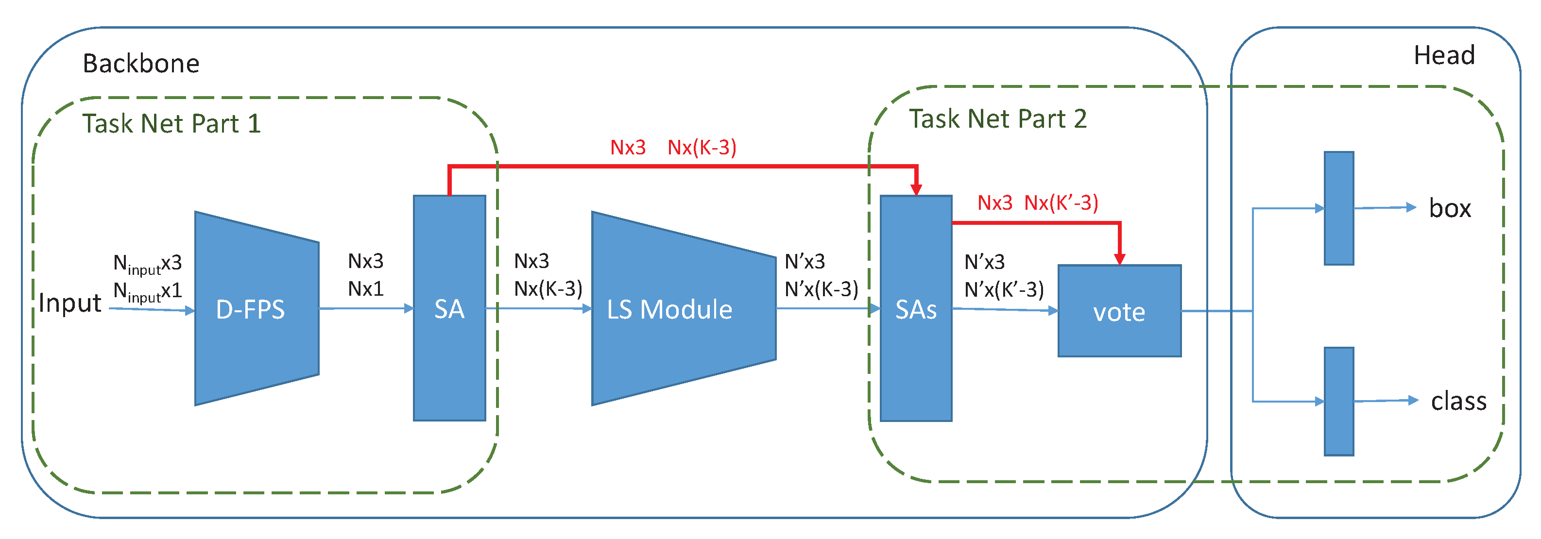
The entire network structure of LSNet is displayed in Figure 2. It is a point-based, single-stage 3D object detection network with a feature extraction backbone and a detection head. The backbone, similar to many other point-based methods [7,29,31,34], uses the multi-scale set abstraction(SA) proposed by PointNet++ [29] to gather neighborhood information and extract features, making it a PointNet-based model as well. Multiple SA modules were stacked to abstract high-level features and enlarge the receptive field. Inspired by VoteNet [31] and 3DSSD [7], a vote layer was added to improve network performance. For downsampling points, the FPS sampling method, i.e., D-FPS in 3DSSD [7], is used to downsample the raw points roughly, while the LS module is used to further sample the points delicately. In addition, there are two 3D detection heads in the proposed model, one for box regression and the other for classification.

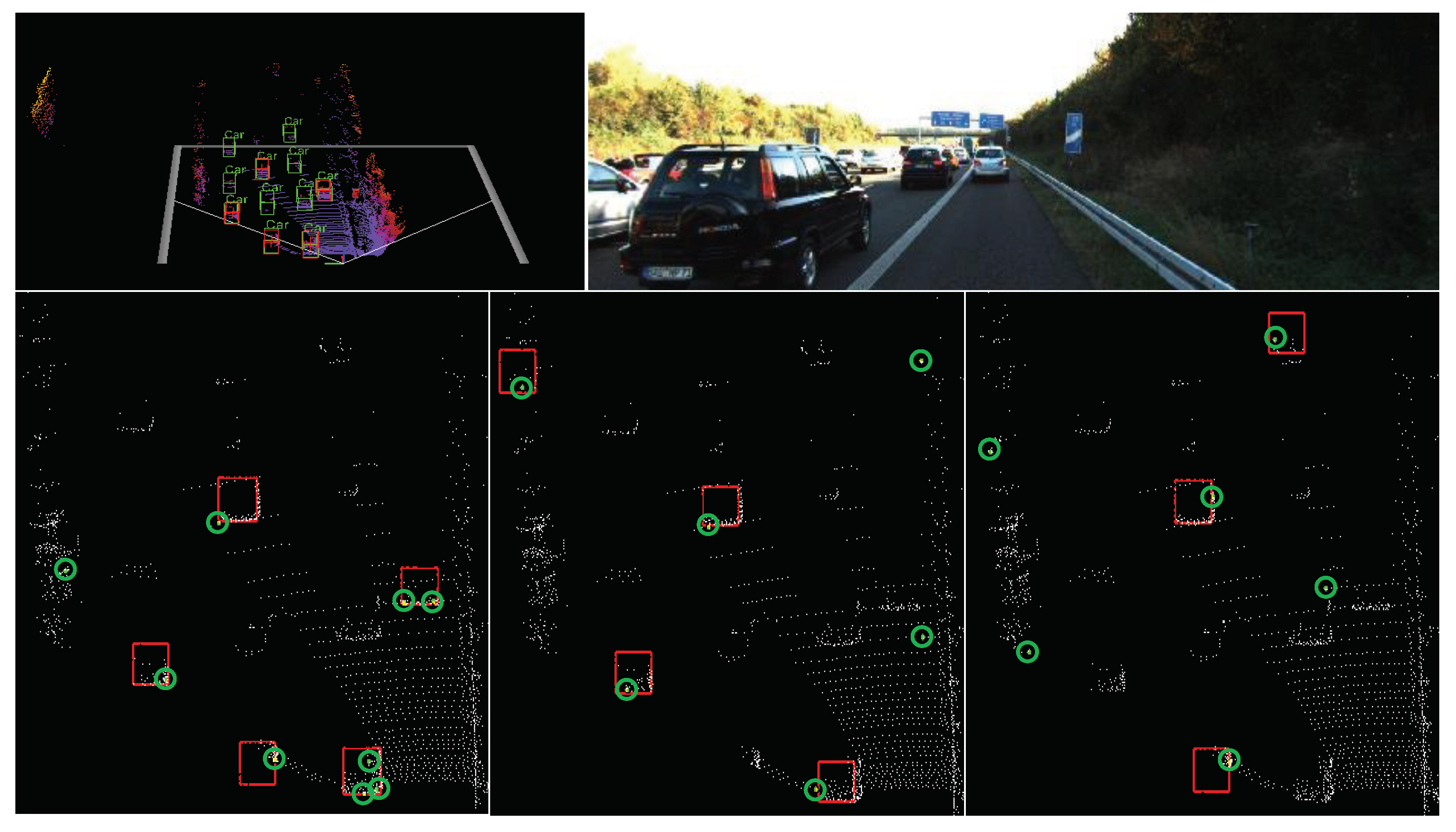
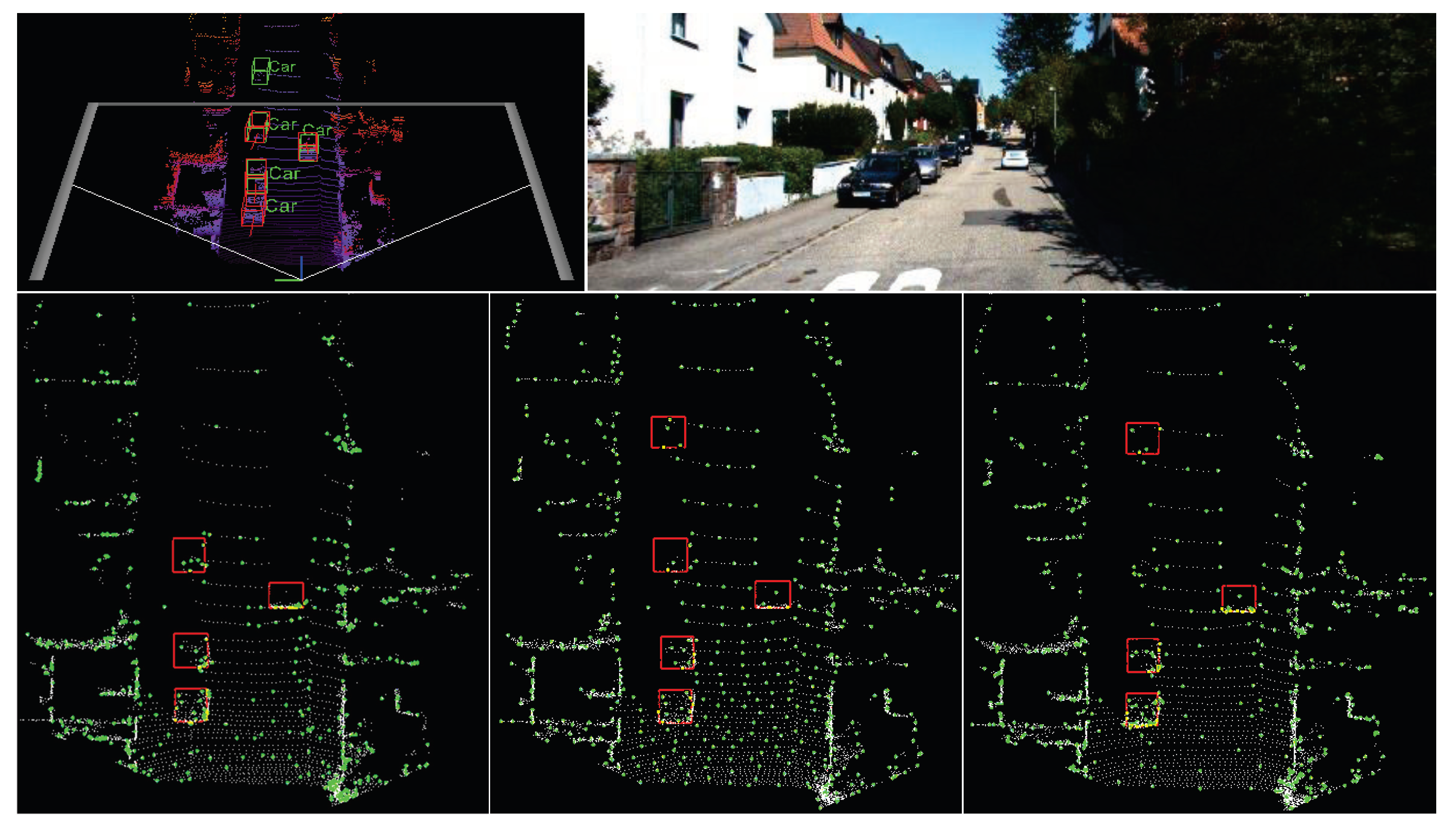
In relation to the LiDAR point cloud, the inputs of the model consist of 3D coordinates and 1D laser reflection intensity, i.e., ${\mathrm{P}}_{input}=\left[{\mathrm{P}}_c{\mathrm{P}}_o\right]$, ${\mathrm{P}}_{input}\in {\mathbb{R}}^{N\times 4},{\mathrm{P}}_c\in {\mathbb{R}}^{N\times 3}$, ${\mathrm{P}}_o\in {\mathbb{R}}^{N\times 1}$. The predicted object in the KITTI 3D object detection dataset can be represented by a 3D bounding box $(c_x,c_y,c_z,h,w,l,\theta )$, including its center, $c_x$, $c_y$, $c_z$, size, h, w, l, and orientation, $\theta$, which indicates the heading angle around the up-axis.

First, FPS based on 3D Euclidean distance is used to sample a subset of the raw points ${\mathrm{P}}_{input}$. Then, the vanilla multi-scale SA module is applied to extract the low-level features ${\mathrm{P}}_o\in {\mathbb{R}}^{N\times \left(K-3\right)}$, which will be viewed as the inputs of the LS module with their coordinates. Working from these middle features, the LS module generates the sampling point cloud ${\mathrm{P}}_{N^{\prime }}$ and ${\mathrm{P}}_{N^{\prime }}\subset {\mathrm{P}}_N$. After several SA modules and a vote layer, the final features are fed into the detection head to predict the box and class of the object. After this, NMS is applied to remove the redundant boxes. Non-maximum suppression (NMS) is a critical post-processing procedure to suppress redundant bounding boxes based on the order of detection confidence, which is widely used in object detection tasks.

According to PointNet++, the SA module has many 1D-convolution-like layers, which are composed of shared-MLP layers. For each point, the SA module groups the surrounding points within a specific radius and uses shared-MLP to extract the features. The box regression head and the classification head are both fully connected (FC) layers.

3.3. LS Module

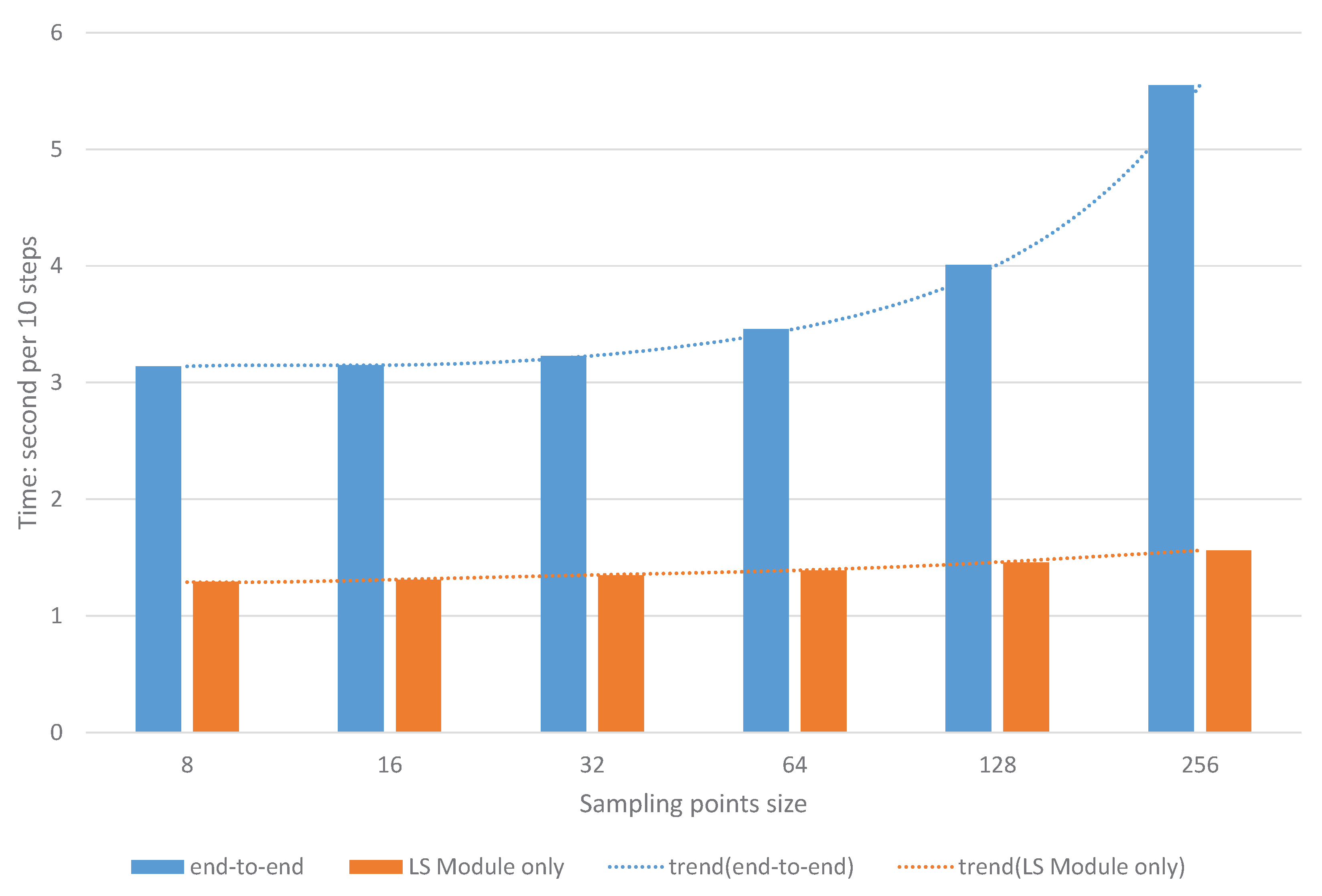
The traditional sampling approaches are neither differentiable nor task-agnostic. Therefore, they cannot be trained using the loss method. Since the sampling process is discrete, we need to convert it to a continuous issue to smoothly integrate the sampling operation into a neural network. Ref. [8] proposed S-Net and [9] proposed its variant SampleNet to ameliorate this shortcoming. These sampling strategies have several defects. First, they generate new point coordinates, which are not in the subset of the original points. In addition, they can only be placed at the beginning of the total network and the entire model lacks the ability to be trained end-to-end. Another issue is due to the fact that the sampling network extracts features from coordinate inputs, while the task network also extracts features from the raw inputs. This duplicated effort inevitably results in a level of redundant extraction in regard to low-level features. A final issue is that the sampling network is relatively complex and time-consuming. This problem will become more severe as the number of points grows. A sampling process that requires burdensome levels of computation to function defeats the purpose of its application to the issue. In consideration of these issues, the discussed methods are not suitable for autonomous driving tasks.

To overcome such problems, the LS module was developed. As illustrated in Figure 3, the network architecture of the LS module has only a few layers, which keeps the complexity low. Rather than extracting useful features to create a sampling matrix from a fresh start, these features are instead extracted by the task network part 1 and are shared, and the matrix is the output based on them to improve computational efficiency and to avoid the repeated extraction of the underlying features.

The input of the LS module is ${\mathrm{P}}_N$, which is the subset of the points sampled by FPS with the features extracted by the former SA module. First a shared-MLP convolution layer is applied to obtain the local feature $F_{local}$ of each point,

$$\begin{array}{c}\hfill F_{local}=f\left(P_N\right|W_1),F_{local}\in {\mathbb{R}}^{N\times k^{\prime }}.\end{array}$$

(10)

Function $f$ represents the shared-MLP convolution layer with its weights W. Then, a symmetric feature-wise max pooling operation is used to obtain a global feature vector $F_{global}$,

$$\begin{array}{c}\hfill F_{global}=MaxPool\left(F_{local}\right)F_{global}\in {\mathbb{R}}^{1\times k^{\prime }}.\end{array}$$

(11)

With the global features and the local features, we concatenate them of each point and pass these features to the shared-MLP convolution layers and use the sigmoid function to generate a matrix $\widehat{S}$, defined as

$$\begin{array}{cc}\hfill \widehat{S}& =f\left(f\left(concat(F_{local},F_{global})\right|W_2)\right|W_3),\hfill \end{array}$$

(12)

$$\begin{array}{cc}\hfill \widehat{S}& =Sigmoid\left(\widehat{S}\right)\widehat{S}\in {\mathbb{R}}^{N\times N^{\prime }}.\hfill \end{array}$$

(13)

$\widehat{S}$ has the same shape as the sampling matrix $\mathrm{S}$. It is the output of the LS module while also being the middle value of $\mathrm{S}$.

To sample data based on ${\mathrm{P}}_N$, the sampling matrix is further adjusted to $\mathrm{S}$ (used in the inference stage) or ${\mathrm{S}}^{\prime }$ (used in the training stage). $\mathrm{S}$ can be computed as

$$\begin{array}{c}\hfill \mathrm{S}=\underset{{\mathbf{p}}_i^{\prime }\in {\mathbb{R}}^N,i\in [1,N^{\prime }]}{one\_hot\_encoding}\left(argmax\left(\widehat{S}\right)\right),\end{array}$$

(14)

where the $argmax$ function and the $one\_hot\_encoding$ function are applied to each column of $\widehat{S}$, i.e., ${\mathbf{p}}_i^{\prime }$ with the shape of original points size N. Since $\widehat{S}$ has $N^{\prime }$ columns, corresponding to $N^{\prime }$ sampled points, and each column of $\mathrm{S}$ is a one-hot vector, Equation (5) can be used to obtain the final sampled points ${\mathrm{P}}_{N^{\prime }}$.

However, the $argmax$ operation and the $one\_hot\_encoding$ operation are not differentiable, indicating that Equation (14) cannot be used in the training stage to enable backpropagation. Inspired by the Gumbel-softmax trick [10,37,38], softmax is applied to each column of $\widehat{S}$ with parameter $\tau$ to approximate the $one\_hot\_encoding$ operation. The generated sampling matrix is called ${\mathrm{S}}^{\prime }$,

$$\begin{array}{c}\hfill {\mathrm{S}}^{\prime }=\underset{{\mathbf{p}}_i^{\prime }\in {\mathbb{R}}^N,i\in [1,N\prime ]}{softmax}(\widehat{S}/\tau ),\end{array}$$

(15)

where parameter $\tau >0$ is the annealing temperature, as $\tau \to 0^{+}$, each column in ${\mathrm{S}}^{\prime }$ degenerates into a one-hot distribution such as $\mathrm{S}$. When the distribution of each column in ${\mathrm{S}}^{\prime }$ does not degenerate to a one-hot distribution, the features of sampled points ${\mathrm{P}}_{o,N^{\prime }}$ are not the same as before. ${\mathrm{P}}_{o,N^{\prime }}$ is computed by the matrix multiplication with ${\mathrm{S}}^{\prime }$,

$$\begin{array}{c}\hfill {\mathrm{P}}_{o,N^{\prime }}={{\mathrm{S}}^{\prime }}^T\otimes {\mathrm{P}}_{o,N},{\mathrm{P}}_{o,N^{\prime }}\in {\mathbb{R}}^{N^{\prime }\times (K-3)};{{\mathrm{S}}^{\prime }}^T\in {\mathbb{R}}^{N^{\prime }\times N};{\mathrm{P}}_{o,N}\in {\mathbb{R}}^{N\times (K-3)}.\end{array}$$

(16)

Nevertheless, it is desirable to keep the coordinates of the sampled points the same as they were previously. So, the $argmax$ operation and the $one\_hot\_encoding$ operation are applied to ${\mathrm{S}}^{\prime }$ to generate sampling matrix $\mathrm{S}$. Then, the coordinates of the sampled points ${\mathrm{P}}_{c,N^{\prime }}$ are computed as

$$\begin{array}{c}\hfill {\mathrm{P}}_{c,N^{\prime }}={\mathrm{S}}^T\otimes {\mathrm{P}}_{c,N},{\mathrm{P}}_{c,N^{\prime }}\in {\mathbb{R}}^{N^{\prime }\times 3};{\mathrm{S}}^T\in {\mathbb{R}}^{N^{\prime }\times N};{\mathrm{P}}_{c,N}\in {\mathbb{R}}^{N\times 3}.\end{array}$$

(17)

Additionally, before Equation (15), a random relaxation trick is employed to further boost the performance of the model, represented as

$$\begin{array}{cc}\hfill \gamma & =r^{\frac{current\_step}{decay\_steps}},r\in [0,1];\hfill \end{array}$$

(18)

$$\begin{array}{cc}\hfill \widehat{S}& =\widehat{S}+Random\left(\gamma \right),Random\left(\gamma \right)\in {\mathbb{R}}^{N\times N^{\prime }},\hfill \end{array}$$

(19)

where r is the decay rate and $\gamma$ is the upper boundary of the random number. Parameter $\gamma$ is decayed with the training step exponentially and eventually approaches 0 when there is no relaxation.

In actuality, the sampling matrix ${\mathrm{S}}^{\prime }$ introduces the attention mechanism to the model. Each column of ${\mathrm{S}}^{\prime }$ indicates the newly generated sampling point’s attention on old points. Then, the new features in ${\mathrm{P}}_{o,N^{\prime }}$ contain the point-wise attention on the old points. Since each column of $\mathrm{S}$ is a one-hot distribution, the coordinates of the sampled points ${\mathrm{P}}_{c,N^{\prime }}$ calculated with $\mathrm{S}$ mean its attention is focused on the single old point when it comes to coordinate generation.

In all the above functions, the shared-MLP function $f$ and the $Sigmoid$ function are point-wise operations, while the random relaxation is an element-wise operation. In addition, the $MaxPool$ function operates from the feature dimension and selects the max value of each feature from all points. This means these functions do not change the permutation equivariance of the LS module. Separate from these functions, Lemma 1 shows the permutation invariance of $softmax$. Thus, our proposed sampling method is permutation-invariant (Definition 1).

3.4. SA Module

The set abstraction procedure proposed by Qi et al., PointNet++, which is widely used in many point-based models, can be roughly divided into a sampling layer, grouping layer, and a PointNet layer. To obtain better coverage of the entire point set, PointNet++ uses FPS to select $N^{\prime }$ grouping center points from N input points in the sampling layer. Based on the coordinates of these center points, the model will gather Q points within a specified radius, contributing to a group set. In relation to the PointNet layer, a mini-PointNet (composed of multiple shared-MLP layers) is used to encode the local region patterns of each group into feature vectors. In this paper, the grouping layer and the PointNet layer are retained in our SA module. The LS module is used instead of FPS to generate a subset of points serving as the grouping center points, while the grouping layer is adjusted to fit our learned sampling model.

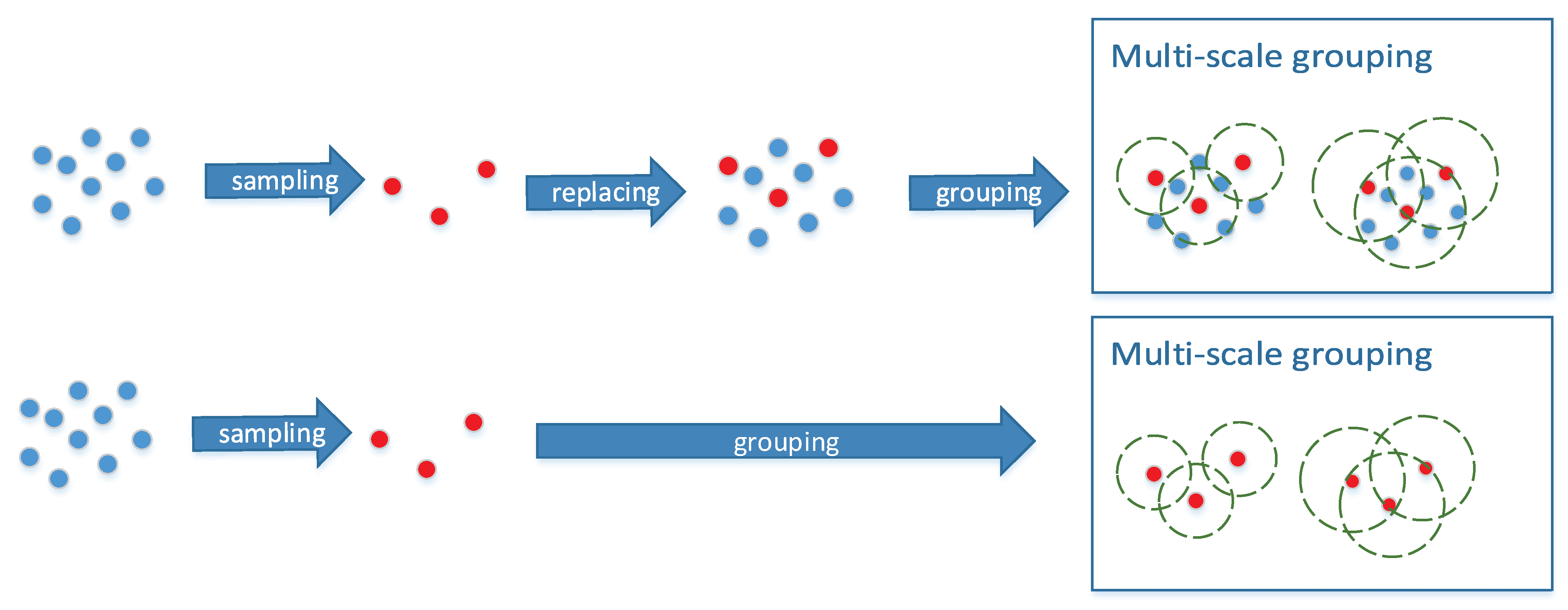
As shown in Figure 4, multi-scale grouping is used to group the points of each center point with different scales. Features at different scales are learned by different shared-MLP layers and then concatenated to form a multi-scale feature. If the points sampled by the LS module are viewed as ball centers and perform the ball grouping process on the original dataset N, similar to PointNet++, the entire network cannot be trained through backpropagation since the outputs of the LS module are not passed to the following network explicitly. Two methods have been developed to address this issue. The first method is to ignore the old dataset before sampling and instead use the newly sampled dataset for both the grouping center points and grouping pool. The other possibility is to use the new sampled dataset as grouping center point and replace the points of the old dataset with the new points in their corresponding positions. Using this method, it is possible to concatenate the features of the new sampled points to each group and pass the outputs (new points) of the LS module to the network.

Within each group, the local relative location of each point from the center point is used to replace the absolute location ${\mathrm{P}}_c$. Importantly, the extracted features ${\mathrm{P}}_o$ will not be affected by shifting or rotating the point cloud. So, it follows that the inputs to the LS module remain the same despite the shift and rotation operations, which also indicates that the proposed sampling method is shift-invariant (Definition 2) and rotation-invariant (Definition 3).

3.5. Loss

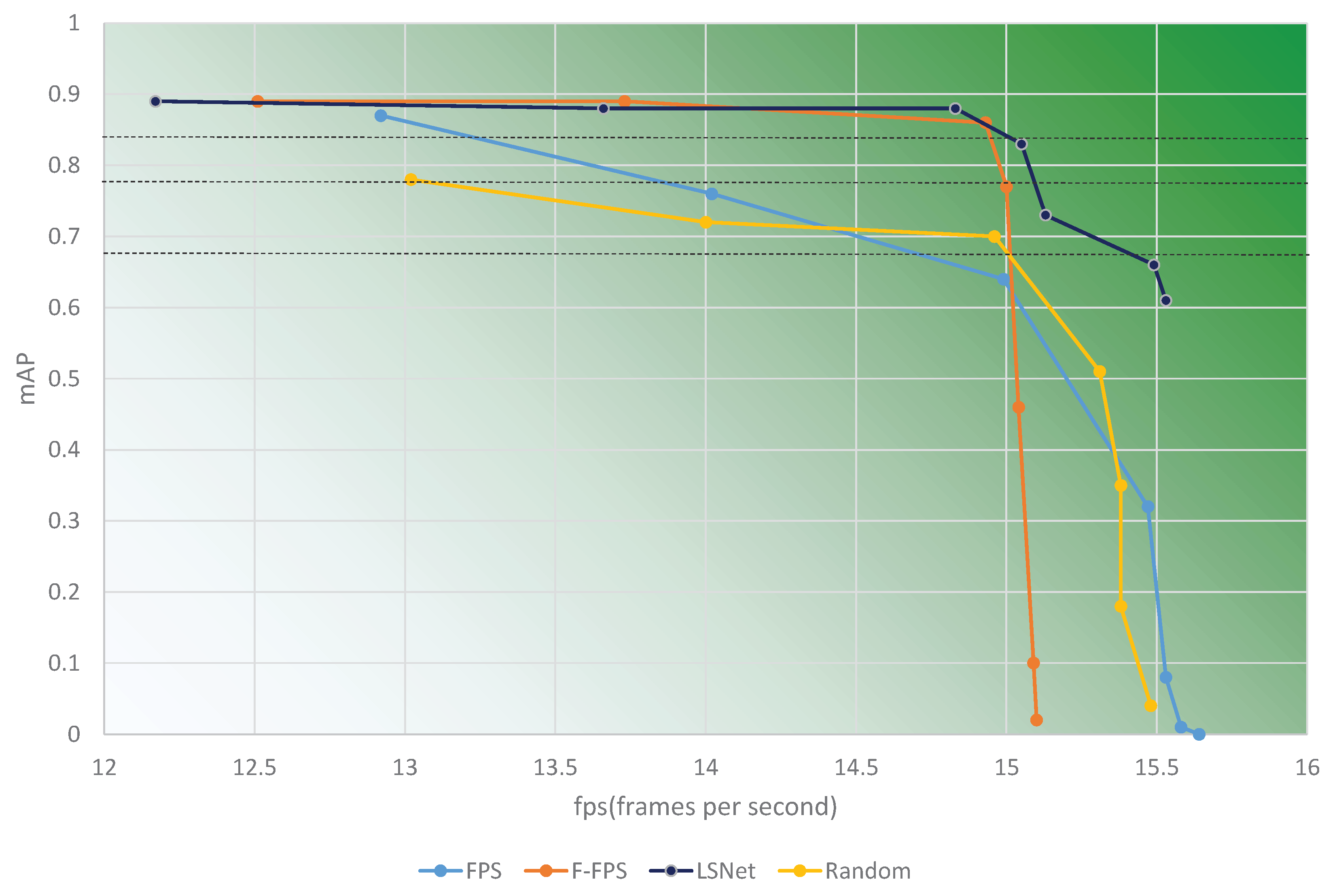
Sampling loss. Unlike the D-FPS and F-FPS methods, the point in the sampling subset generated by the LS module is not unique and the high duplicate rate will result in unwanted levels of computational usage while being unable to make full use of a limited sampling size. This problem increases in severity as the sampling decreases in size.

As illustrated in Equation (20), a sampling loss has been presented to reduce the duplicate rate and sample unique points to as great an extent as feasible. We accumulate each row of ${\mathrm{S}}^{\prime }$, i.e., ${\mathbf{p}}_j\in {\mathbb{R}}^{N^{\prime }}$. ${\mathbf{p}}_j$ represents the sampling value of each point in the original dataset ${\mathrm{P}}_N$. The ideal case is that the point in ${\mathrm{P}}_N$ is sampled 0 or 1 time. Since each column in ${\mathrm{S}}^{\prime }$ can be summarized to 1 and tends to be a one-hot distribution, the accumulation of ${\mathbf{p}}_j$ should tend to be near 0 or 1 if the point is not sampled more than once. Equation (20) is designed to control this issue. The more the accumulation of ${\mathbf{p}}_j$ nears 0 or 1, the less the loss.

$$\begin{array}{c}\hfill L_{sample}=\frac{1}{N}\sum _{j=1}^N\left(\left|\right|\sum _{i=1}^{N^{\prime }}{\mathrm{S}}^{\prime }[j,i]-0.5|-0.5|\right)\end{array}$$

(20)

Each row of ${\mathrm{S}}^{\prime }$ indicates the old point’s attention on the newly generated sampling points. If there are many high values in one row, this old point is highly relevant to more than one new point, and the new point’s features will be deeply affected by the old point with high attention when each column in ${\mathrm{S}}^{\prime }$ tends to be a one-hot distribution. That is, these new points tends to be similar to the same old point, which leads to repeated sampling. However, we expect a variety of new sampling points. In a word, we utilized Equation (20) to restrain each old point’s attention.

Task loss. In the 3D object detection task, the task loss consists of 3D bounding box regression loss $L_r$, classification loss $L_c$, and vote loss $L_{vote}$. ${\theta }_1$, ${\theta }_2$, and ${\theta }_3$ are the balance weights for these loss terms, respectively.

$$\begin{array}{c}\hfill L_{task}={\theta }_1{L}_r+{\theta }_2{L}_c+{\theta }_3{L}_{vote}\end{array}$$

(21)

Cross-entropy loss is used to calculate classification loss $L_r$ while vote loss related to the vote layer is calculated as VoteNet [31]. Additionally, the regression loss in the model is similar to the regression loss in 3DSSD [7]. The regression loss includes distance regression loss $L_{dist}$, size regression loss $L_{size}$, angle regression loss $L_{angle}$, and corner loss $L_{corner}$. The smooth-$l_1$ loss is utilized for $L_{dist}$ and $L_{size}$, in which the targets are offsets from the candidate points to their corresponding instance centers and sizes of the corresponding instances, respectively. Angle regression loss contains orientation classification loss and residual prediction loss. Corner loss is the distance between the predicted eight corners and assigned ground-truth.

Total loss. The overall loss is composed of sampling loss and task loss with $\alpha$ and $\beta$ adopted to balance these two losses.

$$\begin{array}{c}\hfill L=\alpha L_{sample}+\beta L_{task}\end{array}$$

(22)

3.6. Training Method

3.6.1. End-to-End Training

Problem statement: Given a point set ${\mathrm{P}}_N\in {\mathbb{R}}^{N\times K}$, a sample size $N^{\prime }\le N$, and a untrained task network T, find a subset ${\mathrm{P}}_{N^{\prime }}^{*}\in {\mathbb{R}}^{N^{\prime }\times K}$ of $N^{\prime }$ points and a group of weights W of T that minimize the total objective function L:

$$\begin{array}{c}\hfill {\mathrm{P}}_{N^{\prime }}^{*}=\underset{{\mathrm{P}}_{N^{\prime }},W}{argmin}L\left(T\left({\mathrm{P}}_{N^{\prime }}\right)\right|W),{\mathrm{P}}_{N^{\prime }}\subseteq {\mathrm{P}}_N,\left|{\mathrm{P}}_{N^{\prime }}\right|=N^{\prime }\le N.\end{array}$$

(23)

For the end-to-end training method, the task network T and the LS module are trained simultaneously using the total loss L. Compared to the network in the multi-stage training method, the task network part 2 is trained and inferred on the same sampling points distribution. Thus, the entire network is well trained with a certain sampling size.

3.6.2. Multi-Stage Training and Flexibility of the LS Module

Problem statement: Given a point set ${\mathrm{P}}_N\in {\mathbb{R}}^{N\times K}$, a sample size $N^{\prime }\le N$, and a trained task network T, find a subset ${\mathrm{P}}_{N^{\prime }}^{*}\in {\mathbb{R}}^{N^{\prime }\times K}$ of $N^{\prime }$ points that minimizes the total objective function L:

$$\begin{array}{c}\hfill {\mathrm{P}}_{N^{\prime }}^{*}=\underset{{\mathrm{P}}_{N^{\prime }}}{argmin}L\left(T\left({\mathrm{P}}_{N^{\prime }}\right)\right),{\mathrm{P}}_{N^{\prime }}\subseteq {\mathrm{P}}_N,\left|{\mathrm{P}}_{N^{\prime }}\right|=N^{\prime }\le N.\end{array}$$

(24)

Figure 5 shows the flexibility of the LS module and the multi-stage training procedure. The task network part 2 is first trained on sampling points distribution $D_N$. After this, the task network parts are loaded and fixed to train the sampling network(LS module). Therefore, it is possible to obtain a learned sampling points distribution $D_{N^{\prime }}$. Subsequently, in the inference stage, the distribution $D_{N^{\prime }}$ is passed to the task network part 2 for detection. Due to these factors, the task network part 2 is trained and inferred on different sampling points distribution. With the sampled dataset ${\mathrm{P}}_{N^{\prime }}^{*}$ being the best subset of ${\mathrm{P}}_N$ that can make full use of the trained task network, the performance of the network using this method is relatively inferior to the performance of an end-to-end training network because the task network part 2 has not been fully trained with the sampled dataset ${\mathrm{P}}_{N^{\prime }}^{*}$.

In relation to the flexibility of the LS module, the effectiveness of the multi-stage training demonstrates that the LS module can be transferred and adjusted to other point-based models to replace FPS or any other sampling approaches concisely. Even in the case of an already trained task network, point size can still be reduced simply by attaching the LS module to the existing task network and training the LS module solely. This training process can be accomplished quickly because stage 1 is skipped and the LS module is relatively simple and small.

4. Experimental Results

4.1. Setup

Datasets. The KITTI Dataset [12] is one of the most popular dataset for 3D object detection for autonomous driving. All of the experiments for the proposed module are conducted on it. The KITTI dataset collects point cloud data using a 64-scanning-line LiDAR and contains 7481 training samples and 7518 test samples. The training samples are generally divided into the training split (3712 samples) and the val split (3769 samples). Each sample provides both the point cloud and the camera image. Using this approach, only the point cloud is used. Since the dataset only annotates objects that are visible within the image, the point cloud is processed only within the field of view of the image. The KITTI benchmark evaluates the mean average precision (mAP) of three types of objects: car, pedestrian and cyclist. We perform all our experiments on the car objects. Three difficulty levels are involved (easy, moderate, and hard), which depend on the size, occlusion level, and truncation of the 3D objects. For training purposes, samples that do not contain objects of interest are removed.

Data Augmentation. To prevent overfitting, data augmentation is performed on the training data. The point cloud is randomly rotated by yaw $\Delta \theta \sim \mathcal{U}(-\pi /4,+\pi /4)$ and flipped along its x-axis. Each axis is also shifted by $\Delta x$, $\Delta y$, and $\Delta z$ (independently drawn from $\mathcal{N}(0,0.25)$). The mix-up strategy used in SECOND [23] is also used to randomly add foreground instances from other scenes to the current scene. During the translation, it is checked to avoid collisions among boxes, or between background points and boxes.

Network Architecture Details. The network architecture is illustrated in Figure 2. FPS is used to sample 4096 points from the raw input. The LS module will sample points from these 4096 points. There are four multi-scale SA modules in the network with a different shared-MLP structure and a different grouping radius. The shared-MLP layer is a stack of “FC–BN–FC–BN–FC–BN”.

Training and Inference Details. All of the experiments are conducted on a single RTX 2080Ti GPU card. The Adam optimizer [39] is used in the training stage with a learning rate of 0.002. The mini-batch size differs according to each sampling size.

Evaluation Metric. Mean average precision (mAP) is utilized as the evaluation metric. For a fair comparison, the official evaluation protocol is followed. Specifically, the IoU threshold is set to 0.7 for cars. As for the unique rate of the sampled points, this is determined by taking the size of the unique points divided by the size of the entire points.

4.2. 3D Object Detection on the KITTI Dataset

LSNet is evaluated along two points. First is submitting the results of the car objects to the KITTI 3D object detection benchmark and the BEV object detection benchmark.

Table 1. The mean average precision (mAP) comparison of 3D object detection and bird’s eye view(BEV) object detection on the KITTI test set.

Method	Modality	Car-3D (%)			Car-BEV (%)
		Easy	Moderate	Hard	Easy	Moderate	Hard
MV3D [1]	Image + LiDAR	74.97	63.63	54.00	86.62	78.93	69.80
F-PointNet [2]	Image + LiDAR	82.19	69.79	60.59	91.17	84.67	74.77
AVOD-FPN [3]	Image + LiDAR	83.07	71.76	65.73	90.99	84.82	79.62
VoxelNet [24]	LiDAR	81.97	65.46	62.85	89.60	84.81	78.57
PointPillars [25]	LiDAR	82.58	74.31	68.99	90.07	86.56	82.81
SECOND [23]	LiDAR	83.34	72.55	65.82	89.39	83.77	78.59
3DSSD [7]	LiDAR	88.36	79.57	74.55	92.66	89.02	85.86
LSNet (ours)	LiDAR	86.13	73.55	68.58	92.12	85.89	80.80

shows a comparison of the submitted results and the existing literature on the KITTI test dataset. The LSNet-512 (LSNet with 512 sampled points) model is applied to detect the 3D objects of the test dataset, with the results showing that LSNet outperforms other 3D detectors [1,2,3,23,24,25] with only 512 points, and the performance of LSNet-512 is similar to 3DSSD [7] on the easy difficulty level and is a little worse than it on the moderate and hard difficulty levels. For a more specific and detailed comparison of the two models,

Table 2. The mean average precision (mAP) and speed comparison of 3D object detection on the KITTI validation set between 3DSSD and LSNet.

Method	Speed (fps)	Car-3D (%)
		Easy	Moderate	Hard
3DSSD	10.89	90.87	82.62	79.82
LSNet-512	12.17	89.29	78.36	75.46
LSNet-1024	10.71	91.04	82.15	78.98

compares their precision and speed on the KITTI validation set. LSNet-1024 (LSNet with 1024 sampled points) works better than LSNet-512 and shows competitive accuracy compared to 3DSSD. However, LSNet-1024 runs slower than LSNet-512. Although LSNet-512 sacrifices some accuracy, it runs faster than 3DSSD. To balance the accuracy and speed, we chose LSNet-512 as the final model which was used to generate results on the KITTI test set in Table 1.

Second,

Table 3. Performance comparison on the easy difficulty level between different sampling methods on the KITTI validation set. The results are evaluated using the mean average precision (mAP).

Sampled Points	Random (%)	FPS (%)	F-FPS (%)	FS (%)	LS Module (%)
8	4.12	0.18	2.06	0.06	61.28 (+59.67)
16	18.71	1.83	10.87	0.15	66.59 (+58.70)
32	35.95	8.29	46.38	9.09	73.48 (+48.55)
64	51.40	32.61	77.21	45.30	83.57 (+31.94)
128	70.55	64.82	86.63	74.94	88.19 (+13.95)
256	72.81	76.10	89.66	86.10	88.56 (+7.39)
512	78.93	87.75	89.17	85.27	89.29 (+4.01)

,

Table 4. Performance comparison on the moderate difficulty level between different sampling methods on the KITTI validation set. The results are evaluated using the mean average precision (mAP).

Sampled Points	Random (%)	FPS (%)	F-FPS (%)	FS (%)	LS Module (%)
8	3.19	0.18	0.32	0.08	42.49 (+41.54)
16	13.30	2.07	8.57	0.24	46.53 (+40.49)
32	27.11	7.82	35.70	7.56	53.29 (+37.74)
64	39.21	28.60	64.28	34.34	65.18 (+23.57)
128	54.87	54.77	75.87	63.01	72.64 (+10.51)
256	61.20	64.66	79.08	74.72	74.51 (+4.60)
512	66.97	76.79	79.52	76.83	78.36 (+3.33)

and

Table 5. Performance comparison on the hard difficulty level between different sampling methods on the KITTI validation set. The results are evaluated using the mean average precision (mAP).

Sampled Points	Random (%)	FPS (%)	F-FPS (%)	FS (%)	LS Module (%)
8	2.16	0.32	1.31	0.03	33.46 (+32.50)
16	11.76	1.62	7.54	0.28	39.17 (+33.87)
32	24.18	7.49	30.77	6.82	46.28 (+28.97)
64	34.77	26.89	58.65	30.54	58.43 (+20.71)
128	51.20	52.31	71.62	57.05	67.19 (+9.15)
256	57.99	62.84	76.43	70.60	72.63 (+5.67)
512	64.82	73.94	78.83	74.45	75.46 (+2.45)

compare the mAP of different sampling approaches with different sampling sizes. To make a fair comparison, the only change is replacing the LS module with other sampling methods such as random, FPS, F-FPS, and FS sampling, with the rest of the model remaining unchanged. F-FPS and FS are sampling methods raised by 3DSSD [7]. After detailed study about the structure and code of SampleNet, we found that the sampling method of SampleNet [9] is too heavy and not suitable for massive points scenarios such as autonomous driving. Therefore, it is not necessary to conduct experiments on it. The red values between parentheses in these tables are calculated by subtracting the mean of random, FPS, F-FPS, and FS from the value of the LS module. With only eight sampled points, LSNet outperforms other sampling methods significantly with a 60% mAP gain on the easy difficulty level, a 42% mAP gain on the moderate difficulty level, and a 33% mAP gain on the hard difficulty level. Also shown is the fact that when the number of sampling points is decreased, the LS module increasingly outperforms the other approaches. However, once the number of points reaches 512, the differences between these approaches are small. The cause of this behavior is due to the fact that there are already enough points to describe the whole 3D space and the sampling mode does not affect the coverage of key information.

In Figure 6, Figure 7 and Figure 8, visual examples of the described behavior are shown that illustrate the advantages of the LS module. Firstly, by comparing these three sampling methods, we can see that our sampling approach generates more points within the region of interest and near the target object, which is the reason why LSNet works extremely well when the sampling size is small. Furthermore, Figure 6 and Figure 7 depict a complex scene with various features and a simple scene with relatively less different features. It is obvious that FPS and F-FPS performed poorly in the complex scene because there is relatively more distraction. In contrast, our sampling approach can still locate the key areas by selecting the corresponding points nearby.

4.3. Effects of Multi-Stage Training and the Flexibility of the LS Module

As previously described, only the LS module is replaced, with the rest of the architecture remaining the same. This ease of insertion and the removal of the part of the LS module illustrates how flexibly it can be used. Additionally,

Table 6. Multi-stage training on the trained task network with 256 sampled points using the F-FPS sampling method. The first line of the table shows the original performance of the trained model and the results are evaluated by the mean average precision (mAP).

Sampled Points	Easy (%)	Moderate (%)	Hard (%)
256 (task-net)	89.66	79.08	76.43
8	30.19	18.23	14.56
16	42.61	27.13	22.34
32	69.24	50.36	42.28
64	76.47	59.29	50.82
128	84.13	70.08	65.21

and

Table 7. Multi-stage training on the trained task network with 512 sampled points using the F-FPS sampling method. The first line of the table shows the original performance of the trained model and the results are evaluated by the mean average precision (mAP).

Sampled Points	Easy (%)	Moderate (%)	Hard (%)
512 (task-net)	89.17	79.52	78.83
8	6.80	4.36	3.31
16	21.43	15.33	12.52
32	50.31	32.29	26.48
64	64.28	46.47	39.61
128	79.36	52.86	55.31
256	85.58	70.36	66.53

show the results of multi-stage training when starting from an already-trained task network. In this paper, the model trained with the F-FPS sampling approach was used as the task network. Following this, F-FPS was substituted with the LS module. Once the substitution was finished, the weights were set as fixed to solely train the LS module. Finally, Table 6 and Table 7 show the results inferred by the new model with the LS module. Using the LS module, the number of sampled points is halved in short order with only a small loss of accuracy. The number of sampled points of the fixed task model is 256 in Table 6 and 512 in Table 7. This illustrates that the greater the difference in the number of sampled points between the original task network and the LS module, the larger the performance degradation. For example, with 128 sampling points, task-network-256 leads task-network-512 by over 17% mAP gain in moderate difficulty. Figure 9 shows that the training time of the LS module is much shorter in comparison to the time required for the end-to-end training. Furthermore, the growth trend of the time cost for training the LS module is more gentle.

5. Discussion

Ablation Study

In this section, extensive ablation experiments are conducted to analyze the individual components of the proposed approaches. All the models are trained on the training split and evaluated on the validation split for the car class of the KITTI dataset [12].

Effects of the Different Grouping Methods.

Table 8. The mAP results for different groupings.

Sampled Points	Old + New (%)			New Points Only (%)
	Easy	Moderate	Hard	Easy	Moderate	Hard
8	61.24	42.36	33.12	46.49	35.01	29.15
16	66.38	46.09	39.31	69.16	51.61	42.29
32	73.07	53.35	46.21	74.08	57.81	50.26
64	83.47	65.81	58.43	83.13	69.42	63.16
128	88.12	72.42	67.35	87.52	74.16	69.63
256	88.63	74.36	72.61	88.17	74.56	70.47
512	89.36	78.61	75.47	89.35	75.43	72.39

compares the performance between the grouping with the old points and new points together versus the grouping with the new points only. The result is that while there is no difference when the number of points is large, when the number of points is very small, the approach of grouping old and new points together gains higher accuracy. For example, the mAP of eight sampled points for “new points only” is lower than the one for “old + new”, which is caused by the relatively smaller information loss of grouping old and new points together.

Effects of the Sampling Loss. As shown in

Table 9. The effectiveness of sampling loss evaluated by unique rate and mAP results.

Sampled Points	Unique Rate (%)		mAP (%)
	With SL	Without SL	With SL			Without SL
			Easy	Moderate	Hard	Easy	Moderate	Hard
8	95	94	46.49	35.01	29.15	47.35	35.12	30.56
16	95	85	69.16	51.61	42.29	63.26	45.63	39.18
32	95	75	74.08	57.81	50.26	72.53	55.45	49.32
64	95	54	83.13	69.42	63.16	70.64	56.36	50.21
128	96	51	87.52	74.16	69.63	79.10	65.12	60.03
256	96	33	88.17	74.56	70.47	80.59	65.51	60.52
512	95	22	89.35	75.43	72.39	76.53	62.59	56.24

, the proposed sampling loss can boost the unique rate significantly. With our sampling loss, the average unique rate of the points can be stabilized at around 95%. On the contrary, once we remove the sampling loss, the repetition rate climbs to 88% with 512 sampled points and 77% with 256 sampled points. Another issue is that the model performs poorly with a large number of repetition points when it comes to mAP.

Effects of Relaxation.

Table 10. The effectiveness of random relaxation evaluated by mAP results.

Sampled Points	With Relaxation (%)			Without Relaxation (%)
	Easy	Moderate	Hard	Easy	Moderate	Hard
8	61.24	42.36	33.12	54.23	36.19	30.09
16	66.38	46.09	39.31	60.63	41.71	35.32
32	73.07	53.35	46.21	70.52	49.63	44.37
64	83.47	65.81	58.43	81.25	63.61	56.47
128	88.12	72.42	67.35	86.21	70.45	65.21
256	88.63	74.36	72.61	88.04	73.54	71.58
512	89.36	78.61	75.47	88.54	77.31	75.65

confirms that the random relaxation strategy of the sampling matrix yields a higher mAP, i.e., increasing the mAP by an average of 2.96%, 2.94%, and 1.97% on the easy, moderate, and hard difficulty levels, respectively.

Speed Analysis of LSNet. All the speed experiments were run on a 2080Ti GPU.

Table 11. Speed comparison between different sampling methods by checking the fps (frames per second) of the entire model.

Sampled Points	Random	FPS	F-FPS	LS module
8	15.48	15.64	15.10	15.53
16	15.38	15.58	15.09	15.49
32	15.38	15.53	15.04	15.13
64	15.31	15.47	15.00	15.05
128	14.96	14.99	14.93	14.83
256	14.00	14.02	13.73	13.66
512	13.02	12.92	12.51	12.17

illustrates the inference speed of the entire network in fps(frames per second). The processing time of each model with different sampling approaches has little variation, which proves that replacing the original sampling strategy in other models with the LS module will not introduce excessive time consumption. Thus, this shows that the LS module is lightweight and can be plugged into other models without encumbering them. Under the consideration of both inference speed and accuracy, LSNet outperforms the other tested methods according to Figure 10. The green gradient background of the table shows the overall performance of the method, and the darker the color, the better the performance. Then, we can see that LSNet gains higher overall performance, especially when it comes to faster inference speed. Furthermore, we add several auxiliary lines (black dashed lines) in Figure 10 to address this superiority. Each auxiliary line indicates the same accuracy, and LSNet runs faster than other methods with the same accuracy. In addition, FPS collapses very quickly at speeds above 15 fps. The inference time of LSNet-256 is 73 ms and the inference time of LSNet-8 is 64 ms.

6. Conclusions

In this paper, LSNet was proposed to solve the 3D object detection task that operates on LiDAR point clouds. Importantly, the LS module, which is a novel deep-learning-based sampling approach that is differentiable and task-related, was presented. Specifically, with 128 sampled points, it attained a computational acceleration at the cost of acceptable accuracy loss. In addition, the random relaxation method was introduced to the sampling matrix. Evaluated on the challenging KITTI dataset, the LS module of LSNet was found to work extremely well when only using a small amount of sampling data in comparison to the D-FPS and F-FPS methods. The proposed sampling loss was proven to be highly effective in ameliorating the issue of sampling duplicates. Finally, it has been shown that, with an already trained point-based task network, the LS module can be attached to the task network flexibly to replace the original sampling method such as FPS.

As the proposed method has been shown to be superior in comparison to other sampling methods for usage in low sampling size cases and complex scenarios, it is therefore particularly appropriate for autonomous driving usage on urban roads. This is due to the increased complexity faced on urban roads in comparison to highway driving. Additionally, if autonomous vehicles, i.e., trucks, are equipped with multiple LiDARs, this would greatly increase the initial amount of raw points in the system, an issue this sampling method is well suited to handling, giving rise to a reduction in the required memory and computational cost. In a similar vein, the large amount of exploration undertaken recently in China on vehicle-to-everything (V2X) scenarios can also benefit from the LS module. As V2X involves multiple sensors containing LiDAR, they inevitably produce more point cloud data than vehicle-only scenarios. Once again, this means that the module’s efficiency in dealing with such issues is applicable. These varied use cases show the widespread potential and applicability of the LS module.

The LS module tends to sample more points in dense objects than sparse objects, which results in relatively weak performance in moderate and hard categories. In the future, we will work on sampling points evenly on each object and regard their density. Furthermore, it is expected to keep at least one point, even when the object is badly shaded. In addition, we look forward to achieving better accuracy with less points in the following study.

References

1. Chen, X.; Ma, H.; Wan, J.; Li, B.; Xia, T. Multi-View 3D Object Detection Network for Autonomous Driving. In Proceedings of the 2017 IEEE Conference on Computer Vision and Pattern Recognition (CVPR), Honolulu, HI, USA, 21–26 July 2017. [Google Scholar]
2. Qi, C.R.; Liu, W.; Wu, C.; Su, H.; Guibas, L.J. Frustum pointnets for 3d object detection from rgb-d data. In Proceedings of the IEEE Conference on Computer Vision and Pattern Recognition, Salt Lake City, UT, USA, 18–22 June 2018; pp. 918–927. [Google Scholar]
3. Ku, J.; Mozifian, M.; Lee, J.; Harakeh, A.; Waslander, S. Joint 3D Proposal Generation and Object Detection from View Aggregation. In Proceedings of the 2018 IEEE/RSJ International Conference on Intelligent Robots and Systems (IROS), Madrid, Spain, 1–5 October 2019. [Google Scholar]
4. Wang, J.; Zhu, M.; Wang, B.; Sun, D.; Wei, H.; Liu, C.; Nie, H. KDA3D: Key-Point Densification and Multi-Attention Guidance for 3D Object Detection. Remote Sens. 2020, 12, 1895. [Google Scholar] [CrossRef]
5. Hu, Q.; Yang, B.; Xie, L.; Rosa, S.; Guo, Y.; Wang, Z.; Trigoni, N.; Markham, A. RandLA-Net: Efficient Semantic Segmentation of Large-Scale Point Clouds. In Proceedings of the IEEE Conference on Computer Vision and Pattern Recognition, Seattle, WA, USA, 14–19 June 2020. [Google Scholar]
6. Thomas, H.; Qi, C.R.; Deschaud, J.E.; Marcotegui, B.; Goulette, F.; Guibas, L.J. KPConv: Flexible and Deformable Convolution for Point Clouds. In Proceedings of the IEEE International Conference on Computer Vision, Seoul, Korea, 27 October–3 November 2019. [Google Scholar]
7. Yang, Z.; Sun, Y.; Liu, S.; Jia, J. 3dssd: Point-based 3d single stage object detector. In Proceedings of the IEEE/CVF Conference on Computer Vision and Pattern Recognition, Seattle, WA, USA, 14–19 June 2020; pp. 11040–11048. [Google Scholar]
8. Dovrat, O.; Lang, I.; Avidan, S. Learning to sample. In Proceedings of the IEEE Conference on Computer Vision and Pattern Recognition, Long Beach, CA, USA, 16–20 June 2019; pp. 2760–2769. [Google Scholar]
9. Lang, I.; Manor, A.; Avidan, S. SampleNet: Differentiable Point Cloud Sampling. In Proceedings of the IEEE/CVF Conference on Computer Vision and Pattern Recognition, Seattle, WA, USA, 14–19 June 2020; pp. 7578–7588. [Google Scholar]
10. Yang, J.; Zhang, Q.; Ni, B.; Li, L.; Liu, J.; Zhou, M.; Tian, Q. Modeling point clouds with self-attention and gumbel subset sampling. In Proceedings of the IEEE Conference on Computer Vision and Pattern Recognition, Long Beach, CA, USA, 16–20 June 2019; pp. 3323–3332. [Google Scholar]
11. Wu, Z.; Song, S.; Khosla, A.; Yu, F.; Zhang, L.; Tang, X.; Xiao, J. 3d shapenets: A deep representation for volumetric shapes. In Proceedings of the IEEE Conference on Computer Vision and Pattern Recognition, Boston, MA, USA, 7–12 June 2015; pp. 1912–1920. [Google Scholar]
12. Geiger, A.; Lenz, P.; Urtasun, R. Are we ready for autonomous driving? the kitti vision benchmark suite. In Proceedings of the 2012 IEEE Conference on Computer Vision and Pattern Recognition, Providence, RI, USA, 16–21 June 2012; pp. 3354–3361. [Google Scholar]
13. Song, S.; Chandraker, M. Joint SFM and detection cues for monocular 3D localization in road scenes. In Proceedings of the IEEE Conference on Computer Vision and Pattern Recognition, Boston, MA, USA, 7–12 June 2015; pp. 3734–3742. [Google Scholar]
14. Chen, X.; Kundu, K.; Zhang, Z.; Ma, H.; Fidler, S.; Urtasun, R. Monocular 3d object detection for autonomous driving. In Proceedings of the IEEE Conference on Computer Vision and Pattern Recognition, Las Vegas, NV, USA, 27–30 June 2016; pp. 2147–2156. [Google Scholar]
15. Mousavian, A.; Anguelov, D.; Flynn, J.; Kosecka, J. 3d bounding box estimation using deep learning and geometry. In Proceedings of the IEEE Conference on Computer Vision and Pattern Recognition, Honolulu, HI, USA, 21–27 June 2017; pp. 7074–7082. [Google Scholar]
16. Yang, B.; Luo, W.; Urtasun, R. Pixor: Real-time 3d object detection from point clouds. In Proceedings of the IEEE Conference on Computer Vision and Pattern Recognition, Salt Lake City, UT, USA, 18–23 June 2018; pp. 7652–7660. [Google Scholar]
17. Simony, M.; Milzy, S.; Amendey, K.; Gross, H.M. Complex-YOLO: An Euler-Region-Proposal for Real-time 3D Object Detection on Point Clouds. In Proceedings of the European Conference on Computer Vision (ECCV) Workshops, Munich, Germany, 1–4 September 2018. [Google Scholar]
18. Yang, B.; Liang, M.; Urtasun, R. Hdnet: Exploiting hd maps for 3d object detection. In Proceedings of the Conference on Robot Learning, Zurich, Switzerland, 29–31 October 2018; pp. 146–155. [Google Scholar]
19. Li, B.; Zhang, T.; Xia, T. Vehicle detection from 3d LiDAR using fully convolutional network. arXiv 2016, arXiv:1608.07916. [Google Scholar]
20. Chai, Y.; Sun, P.; Ngiam, J.; Wang, W.; Caine, B.; Vasudevan, V.; Zhang, X.; Anguelov, D. To the Point: Efficient 3D Object Detection in the Range Image With Graph Convolution Kernels. In Proceedings of the IEEE/CVF Conference on Computer Vision and Pattern Recognition (CVPR), Virtual, 19–25 June 2021; pp. 16000–16009. [Google Scholar]
21. Chen, Y.; Liu, S.; Shen, X.; Jia, J. Fast point r-cnn. In Proceedings of the IEEE International Conference on Computer Vision, Seoul, Korea, 27 October–3 November 2019; pp. 9775–9784. [Google Scholar]
22. Shi, S.; Wang, Z.; Shi, J.; Wang, X.; Li, H. From points to parts: 3d object detection from point cloud with part-aware and part-aggregation network. IEEE Trans. Pattern Anal. Mach. Intell. 2020, 43, 2647–2664. [Google Scholar] [CrossRef] [PubMed] [Green Version]
23. Yan, Y.; Mao, Y.; Li, B. Second: Sparsely embedded convolutional detection. Sensors 2018, 18, 3337. [Google Scholar] [CrossRef] [PubMed] [Green Version]
24. Zhou, Y.; Tuzel, O. Voxelnet: End-to-end learning for point cloud based 3d object detection. In Proceedings of the IEEE Conference on Computer Vision and Pattern Recognition, Salt Lake City, UT, USA, 18–23 June 2018; pp. 4490–4499. [Google Scholar]
25. Lang, A.H.; Vora, S.; Caesar, H.; Zhou, L.; Yang, J.; Beijbom, O. Pointpillars: Fast encoders for object detection from point clouds. In Proceedings of the IEEE Conference on Computer Vision and Pattern Recognition, Seoul, Korea, 27 October–3 November 2019; pp. 12697–12705. [Google Scholar]
26. Liu, Z.; Zhao, X.; Huang, T.; Hu, R.; Zhou, Y.; Bai, X. TANet: Robust 3D Object Detection from Point Clouds with Triple Attention. In Proceedings of the AAAI Conference on Artificial Intelligence, New York, NY, USA, 7–12 February 2020; pp. 11677–11684. [Google Scholar]
27. Graham, B.; Engelcke, M.; Van Der Maaten, L. 3d semantic segmentation with submanifold sparse convolutional networks. In Proceedings of the IEEE Conference on Computer Vision and Pattern Recognition, Salt Lake City, UT, USA, 18–23 June 2018; pp. 9224–9232. [Google Scholar]
28. Qi, C.R.; Su, H.; Mo, K.; Guibas, L.J. Pointnet: Deep learning on point sets for 3d classification and segmentation. In Proceedings of the IEEE Conference on Computer Vision and Pattern Recognition, Honolulu, HI, USA, 21–27 June 2017; pp. 652–660. [Google Scholar]
29. Qi, C.R.; Yi, L.; Su, H.; Guibas, L.J. Pointnet++: Deep hierarchical feature learning on point sets in a metric space. Adv. Neural Inf. Process. Syst. 2017, 30, 5099–5108. [Google Scholar]
30. Shi, S.; Wang, X.; Li, H. Pointrcnn: 3d object proposal generation and detection from point cloud. In Proceedings of the IEEE Conference on Computer Vision and Pattern Recognition, Long Beach, CA, USA, 16–20 June 2019; pp. 770–779. [Google Scholar]
31. Qi, C.R.; Litany, O.; He, K.; Guibas, L.J. Deep hough voting for 3d object detection in point clouds. In Proceedings of the IEEE International Conference on Computer Vision, Seoul, Korea, 27 October–3 November 2019; pp. 9277–9286. [Google Scholar]
32. Ngiam, J.; Caine, B.; Han, W.; Yang, B.; Chai, Y.; Sun, P.; Zhou, Y.; Yi, X.; Alsharif, O.; Nguyen, P.; et al. Starnet: Targeted computation for object detection in point clouds. arXiv 2019, arXiv:1908.11069. [Google Scholar]
33. Shi, W.; Rajkumar, R. Point-gnn: Graph neural network for 3d object detection in a point cloud. In Proceedings of the IEEE/CVF Conference on Computer Vision and Pattern Recognition, Seattle, WA, USA, 14–19 June 2020; pp. 1711–1719. [Google Scholar]
34. Shi, S.; Guo, C.; Jiang, L.; Wang, Z.; Shi, J.; Wang, X.; Li, H. Pv-rcnn: Point-voxel feature set abstraction for 3d object detection. In Proceedings of the IEEE/CVF Conference on Computer Vision and Pattern Recognition, Seattle, WA, USA, 14–19 June 2020; pp. 10529–10538. [Google Scholar]
35. Liu, Z.; Tang, H.; Lin, Y.; Han, S. Point-Voxel CNN for efficient 3D deep learning. Adv. Neural Inf. Process. Syst. 2019, 32, 965–975. [Google Scholar]
36. Chen, S.; Tian, D.; Feng, C.; Vetro, A.; Kovačević, J. Fast resampling of three-dimensional point clouds via graphs. IEEE Trans. Signal Process. 2017, 66, 666–681. [Google Scholar] [CrossRef] [Green Version]
37. Jang, E.; Gu, S.; Poole, B. Categorical reparameterization with gumbel-softmax. arXiv 2016, arXiv:1611.01144. [Google Scholar]
38. Maddison, C.J.; Mnih, A.; Teh, Y.W. The concrete distribution: A continuous relaxation of discrete random variables. arXiv 2016, arXiv:1611.00712. [Google Scholar]
39. Kingma, D.P.; Ba, J. Adam: A method for stochastic optimization. arXiv 2014, arXiv:1412.6980. [Google Scholar]
Figure 1. The results of different sampling methods processing the same eight sampled points in the same scene. The top-left picture is the 3D object detection results of our model and the green box shows the ground truth, while the red box shows the detection of our model with eight points. The remaining three pictures demonstrate the points before sampling (4096 white points) and the points after sampling (eight green points inside green circle) in the bird’s eye view (BEV). Top-right: sampling results of the LS module, zoomed in and cropped for better illustration since there are no outliers, unlike the other two pictures. Bottom-left: sampling results of D-FPS (FPS). Bottom-right: sampling results of F-FPS.
Remotesensing 14 01539 g001
Figure 2. The overall architecture of the proposed LSNet. The input data of each module contain coordinates data ( N × 3 ) and feature data ( N × K ). The raw coordinates information is kept for point grouping and feature extraction. The blue arrows represent the main data flow of LSNet, while the red arrows demonstrate the data flow in the multi-stage training method when the LS module is skipped. There are two ways to split the entire network for a concise model description in the paper. One is dividing the network into a feature extraction backbone and a detection head. The other is dividing the network into a task network and a sampling network (LS module).
Remotesensing 14 01539 g002
Figure 3. The details of the LS module’s network structure, where B is the batch size, N is the points size, and K is the feature size.
Remotesensing 14 01539 g003
Figure 4. Adjusted multi-scale grouping methods. The red points are sampled by the LS module, while the blue points are old points before sampling. The dotted circle represents a ball of a particular radius. Top: Grouping with old points and new points. Bottom: Grouping with new points only.
Remotesensing 14 01539 g004
Figure 5. Flexibility and multi-stage training. Illustration of the proposed multi-stage training and inference procedure. In stage 1, the LS module is skipped and the task network is trained on N points data with task loss. In stage 2, we use the trained weights from the former stage and fix the weights of the task network layers, after which the LS module is trained through task loss and sampling loss. The LS module will output N sampled points. In stage 3, the inference step, the trained LS module is used to sample data and generate the results.
Remotesensing 14 01539 g005
Figure 6. Visualizing the results of LSNet with 16 sampled points and different sampling approaches. The top-left frame presents the 3D object detection results, where ground truth and predictions are labeled in red and green, respectively. Moreover, the area surrounded by gray lines is the visible area within the image, which can be also recognized as a region of interest. The top-right frame displays the image of the scene. The second line illustrates the sampling results of the LS module, D-FPS, and F-FPS, where the sampled points are displayed in green and the 4096 original points before sampling are displayed in white.
Remotesensing 14 01539 g006
Figure 7. Visualizing the results of LSNet with 16 sampled points and different sampling approaches. This is an easier scene compared to Figure 6.
Remotesensing 14 01539 g007
Figure 8. Visualizing the results of LSNet with 512 sampled points and different sampling approaches.
Remotesensing 14 01539 g008
Figure 9. Time comparison between training the entire model end-to-end and training the LS module only with a batch size of eight.
Remotesensing 14 01539 g009
Figure 10. Speed-precision demonstration of different sampling size and different sampling methods.
Remotesensing 14 01539 g010