Article

Mapping Canopy Cover in African Dry Forests from the Combined Use of Sentinel-1 and Sentinel-2 Data: Application to Tanzania for the Year 2018

1
Joint Research Centre (JRC), Directorate D—Sustainable Resources, European Commission, Via E. Fermi, 2749, I-21027 Ispra, Italy
2
ARHS Developments S.A., 4370 Esch-sur-Alzette, Luxembourg
*
Author to whom correspondence should be addressed.
Remote Sens. 2022, 14(6), 1522; https://doi.org/10.3390/rs14061522
Submission received: 21 January 2022 / Revised: 9 March 2022 / Accepted: 16 March 2022 / Published: 21 March 2022
(This article belongs to the Special Issue Accelerating REDD+ Initiatives in Africa Using Remote Sensing)

Abstract

:
High-resolution Earth observation data is routinely used to monitor tropical forests. However, the seasonality and openness of the canopy of dry tropical forests remains a challenge for optical sensors. In this study, we demonstrate the potential of combining Sentinel-1 (S1) SAR and Sentinel-2 (S2) optical sensors in order to map the tree cover in East Africa. The overall methodology consists of: (i) the generation of S1 and S2 layers, (ii) the collection of an expert-based training/validation dataset and (iii) the classification of the satellite data. Three different classification workflows, together with different approaches to incorporating the spatial information to train the classifiers, are explored. Two types of maps were derived from these mapping approaches over Tanzania: (i) binary tree cover–no tree cover (TC/NTC) maps, and (ii) maps of the canopy cover classes. The overall accuracy of the maps is >95% for the TC/NTC maps and >85% for the forest types maps. Considering the neighboring pixels for training the classification improved the mapping of the areas that are covered by 1–10% tree cover. The study relied on open data and publicly available tools and can be integrated into national monitoring systems.

Graphical Abstract

1. Introduction

The Reduced Emissions from Deforestation and Degradation (REDD+) framework from the United Nations Framework Convention on Climate Change (UNFCCC) is key to addressing climate change and other related environmental emergencies, such as deforestation and forest degradation [1]. REDD+ activities have triggered the need for National Forest Monitoring Systems (NFMS) that produce high-quality, reliable data on forests and forest carbon stocks. The UNFCCC encourages NFMS to use a combination of remote sensing and ground-based forest carbon inventories in order to estimate the greenhouse gas emissions that are associated with forest ecosystems [2,3,4].
In the last ten years, the remote sensing community has witnessed many efforts to produce accurate maps of tree cover and tree cover change with increasing spatial and temporal resolutions. While global initiatives to map tropical forest change do exist [5,6,7], national institutions often look for methods over which they can have complete governance. The current quality, quantity and free availability of remote sensing data is helping to achieve such a goal. In Africa, however, alternative methods are still needed in order to overcome certain limitations and challenges, such as specific technical capacities and skills, computing power and data availability [8].
In the case of East Africa, those limitations add to the already existing challenge of mapping and assessing the tree cover in the dry domain [9,10]. The monitoring of tropical dense moist and boreal forests by optical remote sensing platforms is largely operational [5,6,11,12]; while, in contrast, mapping dry forests with satellite imaginary presents several challenges [10,13]. As illustrated in Figure 1, these challenges include the deciduous nature of the dry forests, the high variation in the structure and canopy cover over time and across biomes as well as a wide range of factors that may distort their aspect as viewed from remote sensing platforms.
As opposed to evergreen forests where the canopy tends to be fully closed, dry forests have a full range of canopy coverage levels, from closed to open. Furthermore, the structure of dry forests is also varied, with the tree cover in open forests (or woodlands) being mixed in different proportions with herbaceous and shrub formations [14,15].
Regarding phenology, dry forests present a mix of phenological characteristics, from semi-deciduous where only a certain proportion of the trees simultaneously loses their leaves through to fully deciduous [16]. During the dry season many of these forests are subject to fires, generally passing through the understory, with burn scars making a major impact on the forest’s level of reflectance. Generally, dry forests are under high anthropogenic pressure from fuel wood collection, charcoal production and grazing, all of which change the structure and composition of the forest canopy and understory [17].
In consequence, dry forests’ reflectance and backscatter, as measured from remote sensing platforms, vary both in time and in space, making the consistent monitoring and discrimination of these dry forests from other land-cover types very challenging, especially through the use of optical data, given the low number of cloud-free acquisitions. Most cloud-free optical satellite images are available in the dry season, a period when these forests have lost their leaves, making them difficult to discriminate from an understory grass layer. Conversely, during the wet season it may be difficult to distinguish a tree layer from shrubs. Despite collecting imagery in all cloud conditions, space-borne synthetic aperture radar (SAR) data have only been used on an ad-hoc basis for forest monitoring until recently, with a test case investigating SAR data’s use in dry tropical forests of Bolivia [18] and another in the humid tropical forests of Central Africa [19].
The increase in the number of available images at a high spatial resolution from 2016 with Sentinel-1 (S1) and Sentinel-2 (S2) allows the use of temporal analysis of reflectance [20] and backscatter [18] for dry forest monitoring. While, for optical data, the increased image acquisition brings the availability of a greater number of cloud-free images and the possibility of temporal analysis of phenology, for SAR data it provides an opportunity to remove the variations in the recorded radar signal due to viewing angles and soil moisture [18]. The potential of combining optical and SAR data has been demonstrated for the mapping and monitoring of the tropical savanna in the Sahel [21,22,23] and it opens new avenues to map and monitor tropical dry forests [24]. It also paves the way for the combined use of S1 and S2 or Landsat-8 time series through data fusion [25].
The exploitation of these large data volumes has been made possible by the development of cloud-based computing capacities with a range of classifiers, allowing rapid processing [26]. Cloud computer processing and machine learning techniques are now becoming the norm for extracting meaningful information from terabytes of satellite images [27,28]. However, there is a learning and technological gap for many of the users in the field [29]. A transition from image interpretation methods to more advanced big data processing is needed. A successful way to operate that transition is to create user-flexible methods with different levels of uptake from the users [30].
The main objective of this present study is to demonstrate the potential of open Copernicus data, namely S1 and S2, for the national-scale mapping of dry tropical forests in the framework of REDD+. First, we explored what is the best period in which to handle the seasonality and the availability of the S2 data and we evaluated the benefit of S1 data. Second, an expert-based data collection was performed that resulted in a training dataset that was suitable for dry forest monitoring applications with Earth observation (EO) data. Third, different classification models and approaches to incorporate the spatial information into the models were tested. In order to support the work that is done by NFMS, we share the scripts for processing the satellite imageries, the resulting maps and the expert-based reference dataset.

2. Study Area

The study area covers the United Republic of Tanzania. To consider the potential discrepancies in the country’s boundaries, we considered a polygon encompassing a buffer zone of approximately 40 km from the national boundary of Tanzania.
Tanzania lies in Eastern Africa, bordering the Indian Ocean, between Kenya and Mozambique and covering a land area of 945,087 square kilometers. Tanzania has a tropical climate with regional variations due to its topography. A central highland of around 900–1800 m is covering the major part of the country, including the Kilimanjaro mountain range with its highest peak of 5895 m [31].
Regarding precipitation, the country has a complex seasonality with a mix of bimodal and unimodal rainfall patterns. The south western and central parts of Tanzania have one rainy season from December to April. The north-east of the country, except Lake Victoria, receives rainfall in two periods, from October to December and from March to May. In the area of Lake Victoria, a long rainy season usually lasts from October to May. The west of the country, bordering Lake Tanganyika, has one rainy season from November to April [32].
Agricultural land covers more than 43% of the country’s area and forests cover up to 37%. While agriculture and forestry are both important components of Tanzania’s economy, agriculture contributes to the gross domestic product to a much larger extent than the forests do. This might change in the future as the forests’ exploitation share is increasing significantly [33]. Tanzania possesses a range of forests with different structures, canopy cover and phenology; evergreen montane forests [34], semi-evergreen coastal forests [35] and dry miombo forests [36]. Despite conservation efforts, more than 5.86 million hectares of Tanzania’s forests were lost due to deforestation and degradation between 2000–2015. That represents approximately 10% of the country’s forests overall [37]. As bioenergy provides more than 90% of the country’s energy needs, the main cause of the forest loss is charcoal production [33].

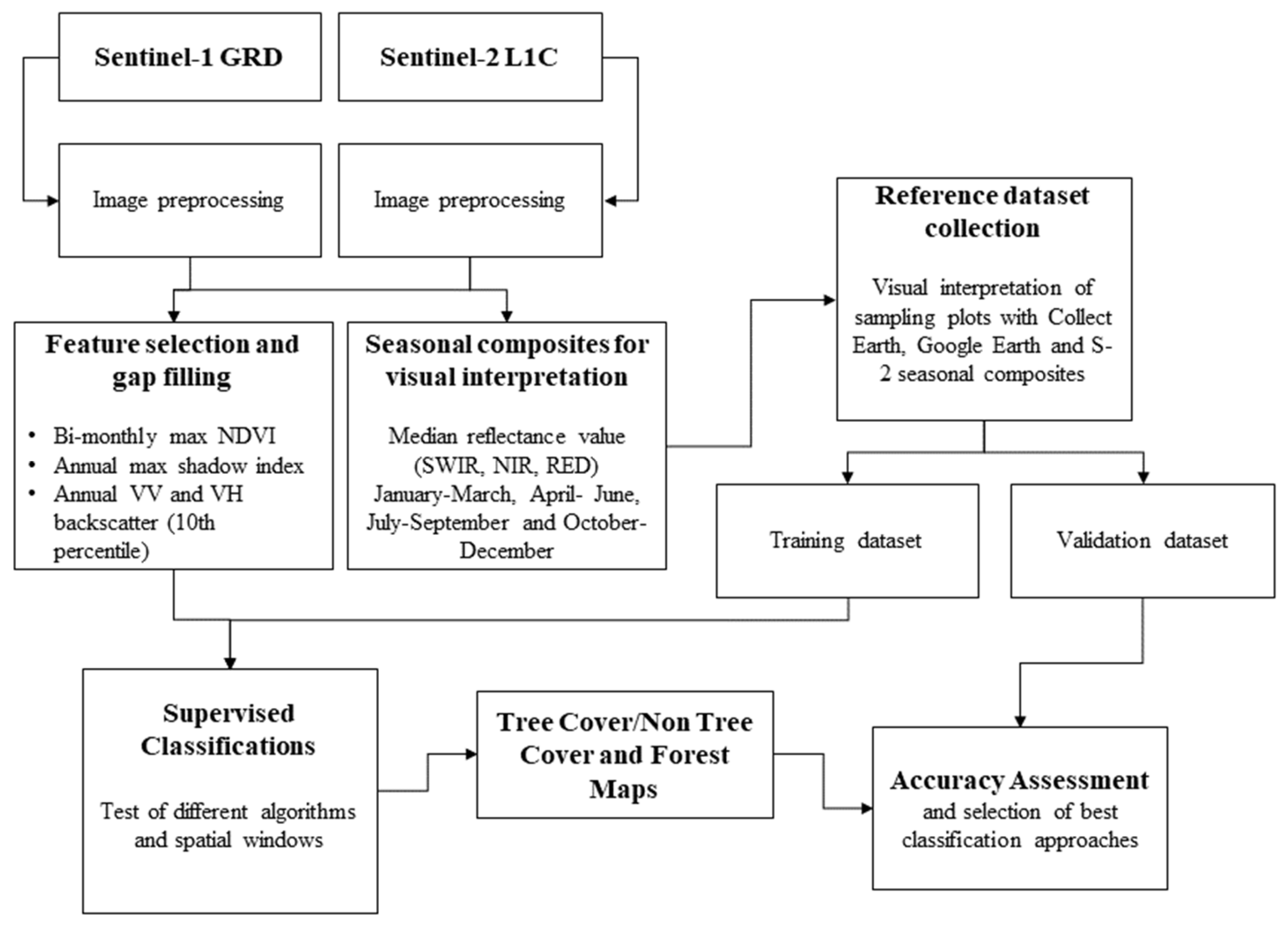
3. Materials and Methods

The overall methodology consists of three main steps, which are presented in Figure 2: (i) the generation of the S1 and S2 layers, (ii) the collection of an ad-hoc training/validation dataset and (iii) the classification of the data. In this study, we tested three supervised classification algorithms and evaluated their suitability for the mapping of dry tropical forests. Additionally, different approaches to incorporate the spatial information in order to train the classifiers were explored. The following sections describe the steps of the methodology that was developed.

3.1. Sentinel-1 and Sentinel-2 Layers

The first step of the methodology was the processing of the S1 and S2 data into layers that are relevant for dry forest monitoring. The data were processed on the Google Earth Engine (GEE, [26]) platform. For the processing of the initial selection of the S1 and S2 image tiles, a buffer of 100 km was added to the study area’s polygon in order to include those tiles that do not have their centroid inside the initial polygon.

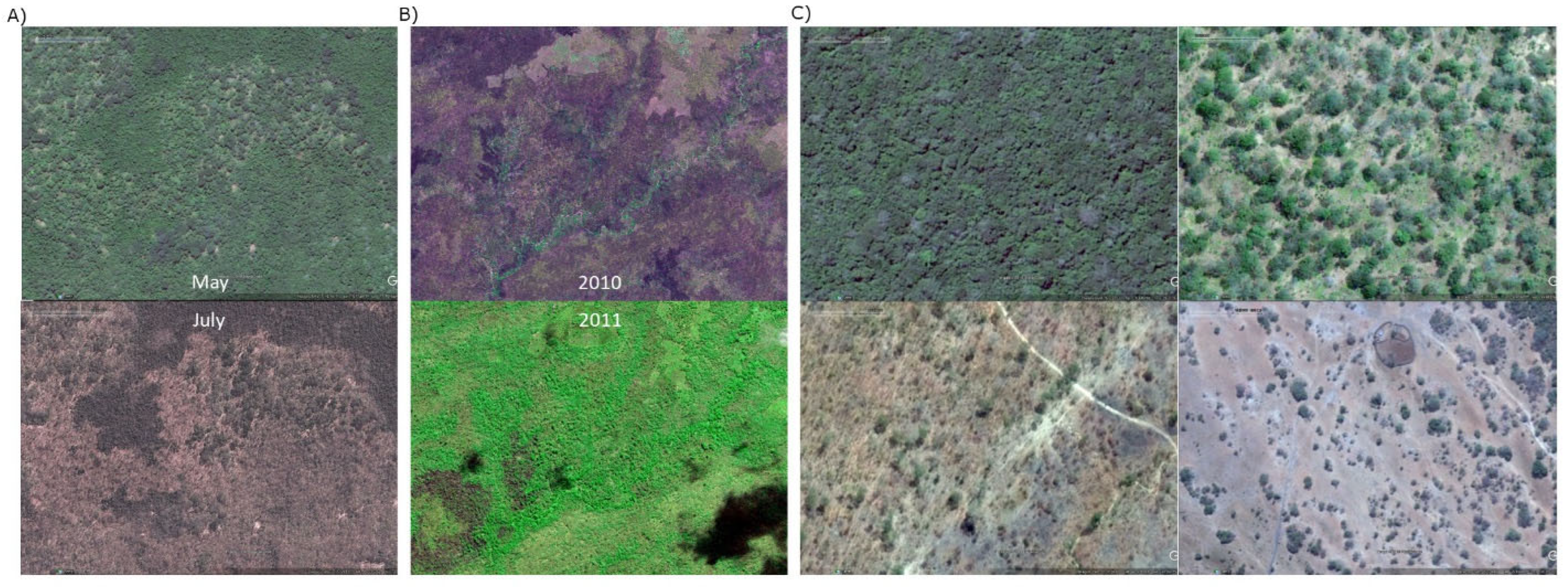
3.1.1. Optical Data: Sentinel-2

S2 satellites carry a wide-swath, high-resolution Multispectral Instrument (MSI) with 13 spectral bands spanning from the visible to the short-wave infrared. The spatial resolution varies from 10 m to 60 m depending on the spectral band. The swath is 290 km. The temporal resolution of the S2A satellite is 10 days [38]. The S2A satellite was launched on the 23 June 2015. A revisitation period of five days at the equator is ensured by the launch of the S2B twin satellite on the 7 March 2017.
All of the available S2 Level 1C (L1C) top of atmosphere (TOA) reflectance scenes on the GEE platform for 2018 over Tanzania were used. The year 2018 is the first year with a complete coverage from S2A and S2B. The top of canopy reflectance products (Level-2A) were only in the process of being ingested into the GEE system for the year 2018 at the time of the processing. While surface reflectance is preferred across the literature, atmospheric correction is not always a prerequisite for classification applications [39]. Furthermore, the classification was based on the vegetation indices (VI) that reduce the atmospheric effects.
A custom cloud and shadow masking was applied to the L1C single images. The cloud masking was an adaptation of the cloud-score that was developed by [40] for Landsat 8 and used by [41]. A higher cloud-score was assigned to pixels with (i) higher brightness in the blue and cirrus bands (S2 bands 1, 2 and 10); (ii) higher brightness in all of the visible bands (bands 2 to 4) and (iii) higher normalized difference water index (NDWI) value. The NDWI was calculated with S2 bands 8 and 11 [42]. Any pixel with a cloud-score that was higher than 40 was considered to be cloud-contaminated.
Two VIs were selected, the normalized difference vegetation index (NDVI) and the shadow index (SI) [43]. The NDVI highlights the seasonal behavior of the vegetation while the SI was used as a proxy for the forest canopy’s density.

NDVI Bi-Monthly Time Series

NDVI is commonly used as an indicator of the status of vegetation due to its sensitivity to photosynthetically active biomass and the phenological dynamics that are present in the vegetation [44]. The seasonal variation of the vegetation is captured following the yearly evolution of the NDVI. However, a trade-off between the length of the compositing period and the availability of non-cloudy data had to be found. Despite a 5 day acquisition scheme, it was difficult to build S2 composites at a country level that were shorter than two months since the cloud coverage was too impactful during the rainy season. Figure 3 shows the number of cloud-free observations for each bi-monthly period.
First, the NDVI was calculated for each single image using Equation (1). Second, the maximum value was retained for a two-month period.
NDVI = (NIR − RED)/(NIR + RED)
where NIR is band 8 and RED is band 4 of S2.
All of the layers were exported in the scale of 8-bits, adding +1 to the NDVI continuous value and multiplying by 100, which resulted in values from 0 to 200.

Shadow Index

The second vegetation index that was used is the SI. The SI rises as the forest density increases; i.e., young and evenly spaced trees have a low canopy shadow index compared to mature natural forest stands [43]. A study by [45] highlighted SI as a strong explicative factor in aboveground biomass prediction from remote sensing biophysical parameters.
The SI was calculated with the Equation (2) on cloud-masked images. To eliminate the extreme values, the 90th percentile over the monthly SI was applied as a cut-off value. Then, the maximum value among the 12 months was retained.
SI = ( ( 1 BLUE ) × ( 1 GREEN ) × ( 1 RED ) ) 1 / 3

Composite for Visual Interpretation

In addition to the VIs, four composites were created for visual interpretation purposes. The median reflectance values for a three month period were computed from the cloud-masked S2 images for band 4 (Red), band 8 (NIR) and band 12 (Swir~2190 nm).

3.1.2. SAR Data: Sentinel-1
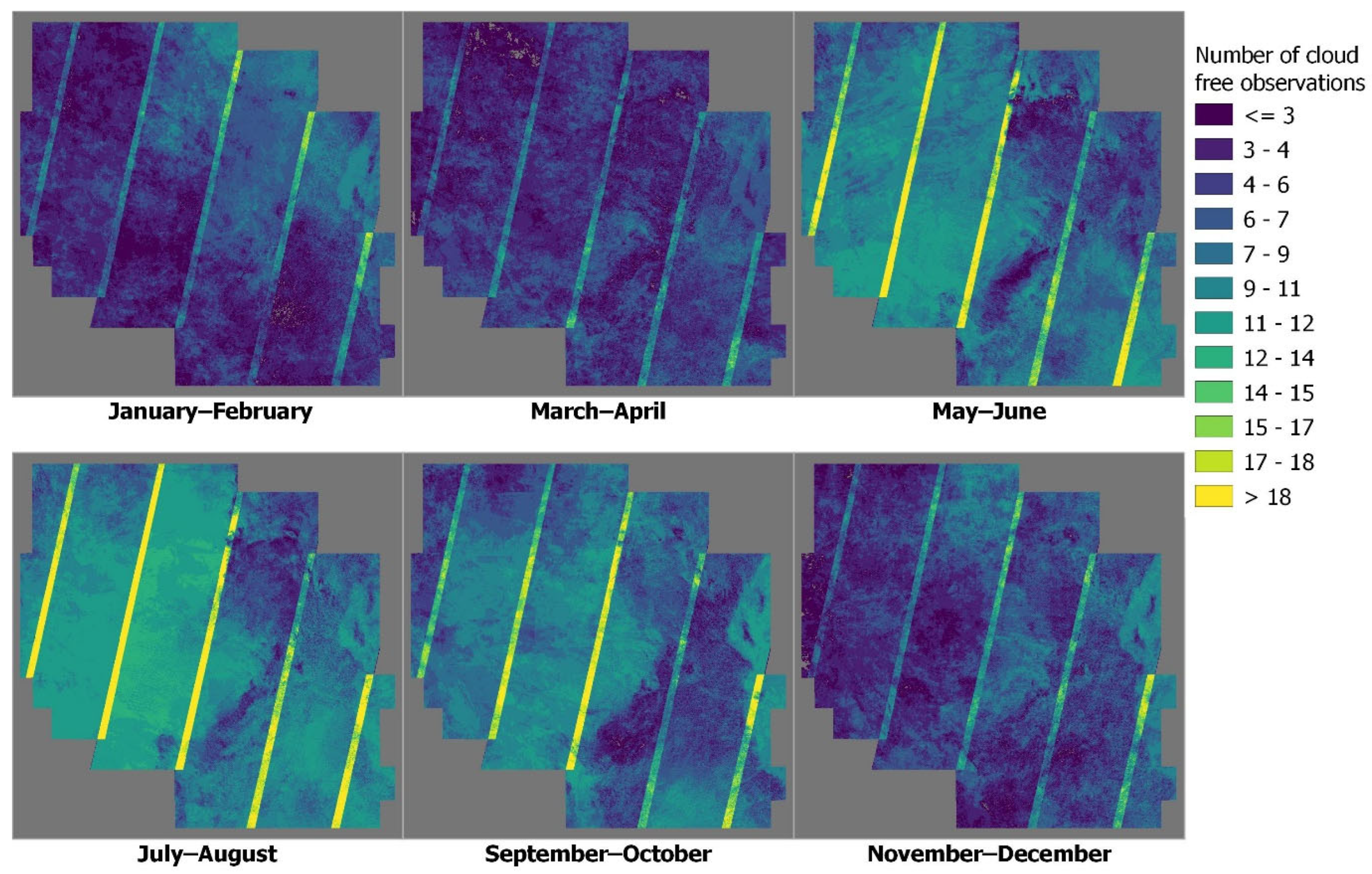
S1 satellites carry a C-SAR sensor, which offers medium and high resolution [46]. The C-band SAR instrument supports operation in single polarization (HH or VV) and dual polarization (HH + HV or VV + VH). S1 is a two-satellite constellation (S1A and S1B) with a revisit-frequency over Africa of 12 days. Considering the overlap and combining the ascending and descending orbits, this leads to a S1 observation every ~4 days [47].
We used all of the S1 tiles that were acquired in the interferometric wide (IW) swath mode, providing dual-polarization (VV and VH) in both the ascending and descending orbits, that were available in GEE for 2018 over Tanzania. In GEE, the Level-1 Ground Range Detected (GRD) IW product is processed with the S1 Toolbox [48] for thermal noise removal, radiometric calibration and terrain correction and projected onto a regular 10 m grid.
The understanding of the backscattering variation of a C-band wavelength in its interaction with deciduous trees’ phenological changes is still in its early stages [49,50]. The knowledge for Eastern African dry forests is even more limited. The C-band of S1 interacts with elements of an approximate size of 5 cm. For trees, the dominance of the crown return with the C-band is stronger than with lower frequencies, such as S- or L- band [50].
The temporal profiles in VV and VH polarization (Figure 4) show that pixels covered by trees tend to have higher backscatter values throughout the year, while open land presents more variation. For instance, agriculture land presents a decrease in the backscatter intensity during the dry season. One hypothesis is that the tree, even without leaves, is still interacting strongly with the signal while open land only leads to a stronger backscatter signal when herbaceous vegetation is present. An annual minimum value, not contaminated by noise, is likely to highlight the tree cover’s presence inside a pixel. Accordingly, the full 2018 time series was decomposed into bi-monthly composites for each polarization, VV and VH. The 10th percentile was retained for two months and filtered with a Lee filter. Then, the minimum value over the 6 bi-monthly composites was retained for each polarization.

3.1.3. Gap Filling

A total of 9 layers were used as the final input for the classification models (Table 1). The layers that were not highly correlated and heavily affected by noise or missing data were selected and downloaded from GEE. Despite the careful selection, the S2 layers contained some missing data. As missing data are not correctly handled by machine learning classifiers, a gap-filling procedure was applied on the six NDVI layers prior to the classification workflow. The missing values were filled by combining the median value over an incremental spatial window with the maximum NDVI value over the 6 bi-monthly composites. The average value resulting from the two approaches was used to fill in the gaps.

3.2. Reference Dataset Design

Field data describing the dry forests in East Africa are generally very sparse on the large scale due to location and accessibility limitations. In addition, field data are usually not designed for EO applications, which require homogenous polygon-based data (i.e., data that are not referred to a single point). In Tanzania, an NFI commonly named National Forest Resources Monitoring and Assessment (NAFORMA) was carried out from 2009 to 2014 by the Tanzania Forest Services [51,52], which provided ground-based data related to forest biomass. However, the field data can exhibit inconsistencies in terms of the data collection and a lack of precision of the GPS coordinates. In order to extract the information that is related to dry forests from S1 and S2, we therefore created a training dataset which was suited to this study as well as to other broader applications.

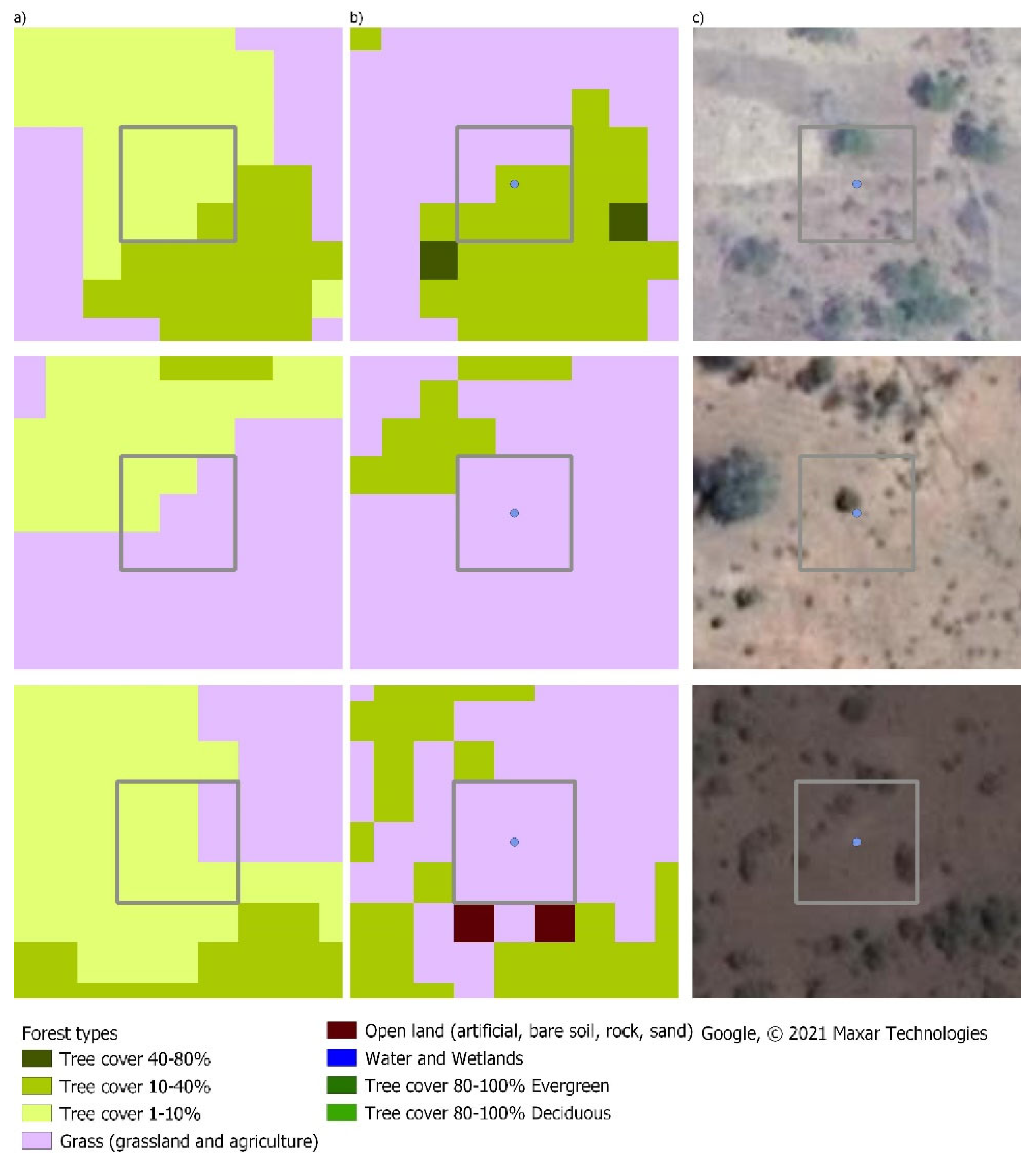
3.2.1. Classification Legend

A multi-level legend is proposed in Table 2. The first step was to gather the information on the presence of tree cover, single trees or the absence of woody vegetation (Level 0 in Table 2). Any woody element with a height of over 3 m was considered to be a tree. The second step was to categorize the canopy cover into four categories (Level 1 in Table 2): 80–100% canopy cover, corresponding to a closed evergreen forest or bushland; 40–80% canopy cover, corresponding to a closed woodland or bushland; 10–40% canopy cover, corresponding to an open woodland or bushland and 1–10% canopy cover, representing a landscape that is covered by grassland or agriculture and single isolated trees. The third step was to document some of the characteristics that are specific to the type of woody vegetation that was present (Level 2 in Table 2). For the 80–100% class, the distinction between evergreen or semi-evergreen and deciduous trees was made.

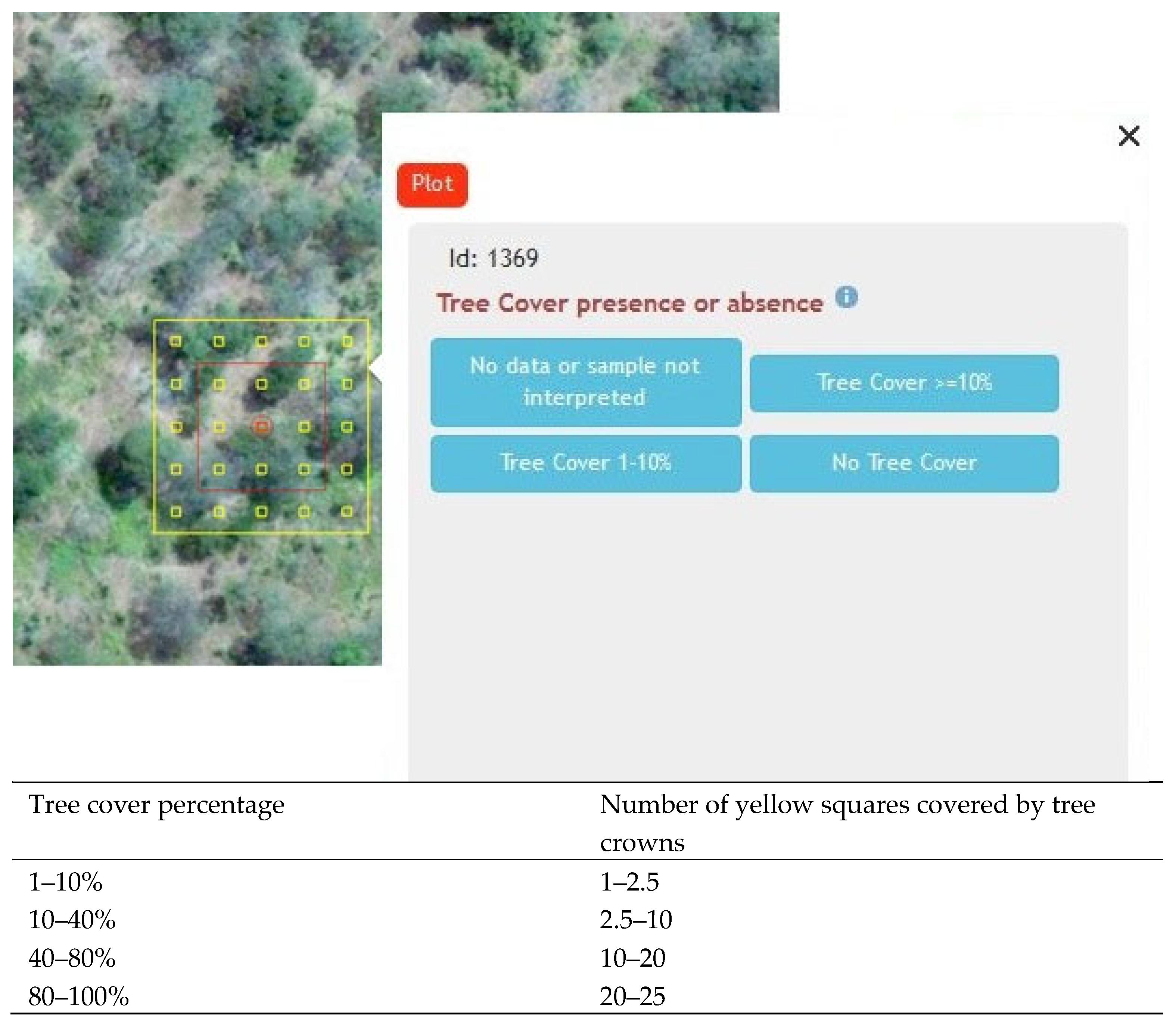
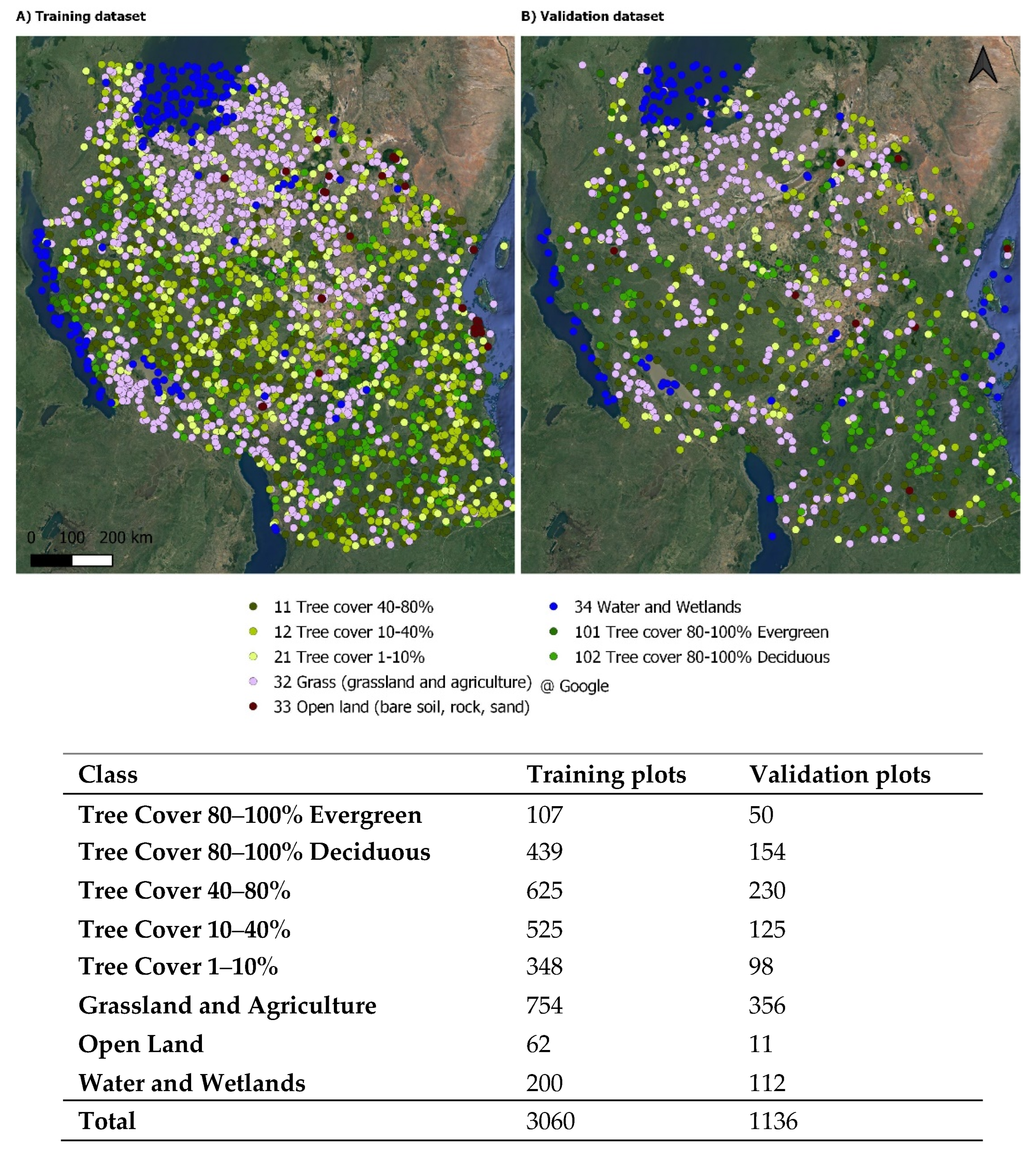
3.2.2. Sampling and Response Design

The marked plots were distributed through a random stratified sampling that was derived from a vegetation–non vegetation stratification based on an S2 annual maximum NDVI composite. The sampling for the validation process was additionally fine-tuned based on the classification results using the recommendations for adjusting for classes that were less-represented in the map [53].
The samples of the reference dataset were collected by the visual interpretation of very high resolution (VHR) images from Google Earth with the free and open-access software tool Collect Earth [54]. Collect Earth, a tool developed by the UN-FAO for the monitoring of land cover and land use, is a state-of-the-art technique for the visual interpretation of VHR images [55]. Collect Earth allows for the collection of plot-level information using various sources of remote-sensing data. Built on Google Earth technologies, it provides access to all of the available satellite archives of VHR images [55]. It also facilitates access to Bing Maps’ collection and enables multi-user interpretation.
The interpretation was performed on a square plot of 0.25 ha, corresponding to 25 S2 pixels at a 10 m resolution. In order to take into account the possible shift from the Google Earth and Bing images with the S2 and S1 images, the classification considered the 9 central pixels of the square plot, equivalent to an area of 0.09 ha.
Various tests showed that a visual distinction between trees and shrubs could not be carried out consistently on the country scale solely on the basis of the VHR imagery. Indeed, the presence of multiple stems and the height of the woody element are two discriminant features that are commonly used to differentiate between trees and shrubs when collecting field data, but these parameters cannot be retrieved from optical remotely-sensed VHR imagery. It was therefore decided that any woody element having a crown of at least 5 m in the 0.25 ha window would be interpreted as a tree element. For the visual interpretation, tree cover was defined hereafter as a woody element with a canopy crown ≥ 5 m in diameter and a height of more than 3 m (these are features that cannot be seen on the VHR images). As illustrated in Figure 5, the interpreter visualizes a 0.25 ha square plot, a 0.09 ha central square plot and a circle of 5 m diameter around the central point. The circle is there indicating the 5 m tree crown threshold that is fixed to discriminate woody vegetation. The four categories of tree cover were evaluated according to the number of yellow squares that were covered by tree canopies. In addition to the VHR image archives that are available in Google Earth and Bing Maps, the interpreter had access to the S2 composite for the year 2018. The composite was displayed with the three bands which are useful in the context of forest monitoring (band 11 SWIR 1, band 8 NIR and band 4 RED). To document the seasonality of the 80–100% plots specifically, NDVI profiles from Landsat 8 and MODIS were provided through a script running on the GEE platform.
Only plots with a VHR image that was available from close to year 2018 in Google Earth or Bing were interpreted. The interpreter also discarded any plot that did not present homogeneous vegetation cover in the 0.25 ha square (e.g., plots at the border of a forest). A total of 4196 plots were interpreted with a sufficient level of confidence (split between 3060 plots for training and 1136 for validation—Figure 6).

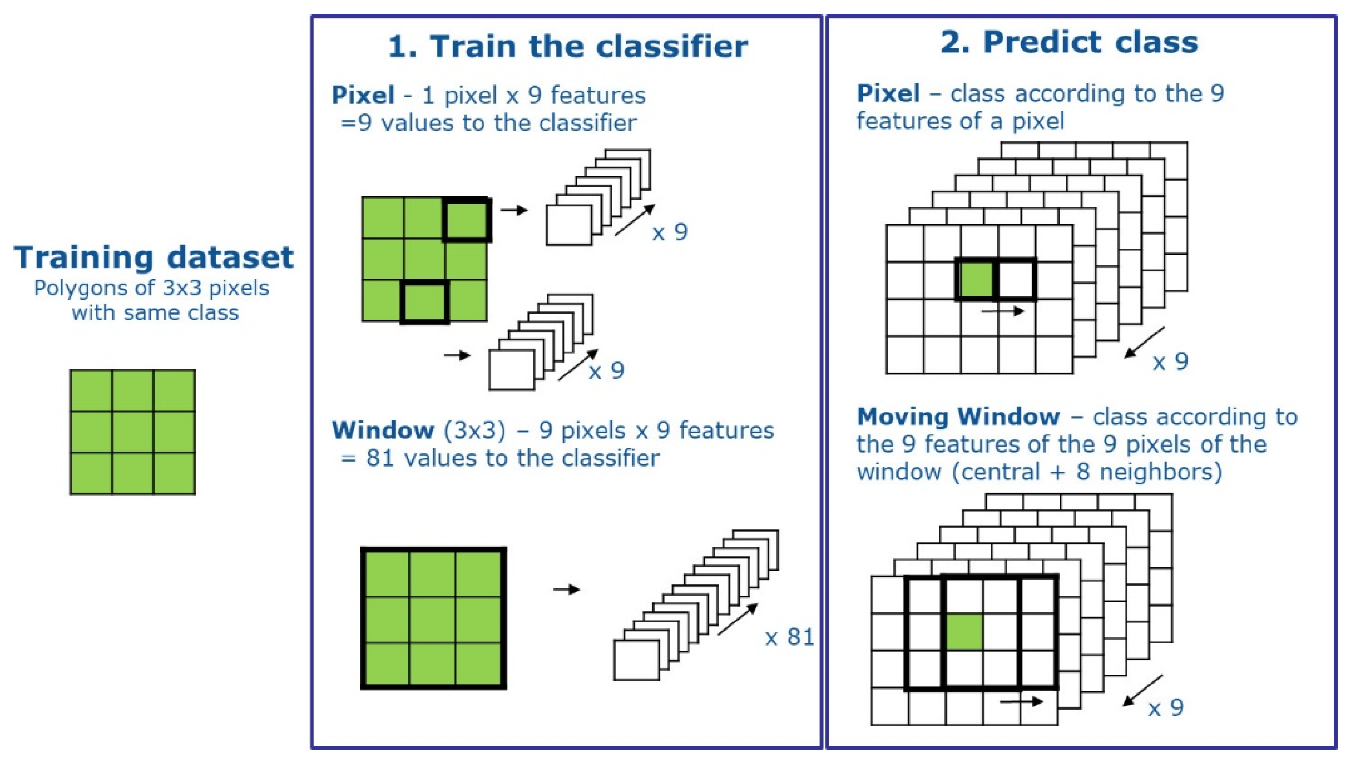
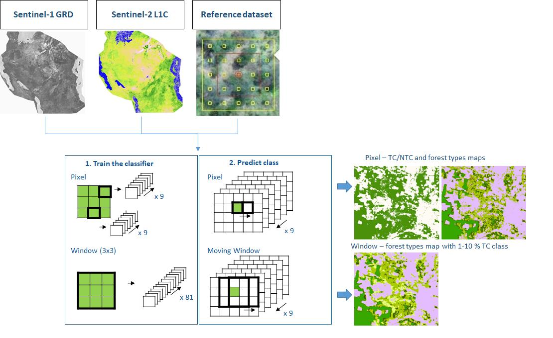
3.3. Classification Workflows

The presence of tree cover and the distribution of the forest types at a national level were predicted through three different classification workflows. From the training dataset, Level 0 of Table 2 was used in order to predict the binary presence or absence of tree cover, while Level 1 was used to predict the different levels of canopy cover. For closed canopy cover, we distinguished between tree cover from evergreen and deciduous forests (classes 101 and 102 from Level 3).
The classification was done based on the 3 × 3 pixels central plot from the 5 × 5 pixels that were interpreted for each plot. The 9 annotated pixels from the central plot were used into two different thematic mapping approaches: the first approach, called “pixel” in Figure 7, classified the pixels into classes according to their intrinsic spectral values, while the second approach, called “window” in Figure 7, used a contextual spectral approach to classify the pixels while also considering their neighboring pixels.
The binary tree cover–no tree cover discrimination was trained with the “pixel” approach only; that is, the 9 pixels were considered as 9 independent training samples. For the classification of the canopy cover classes, both approaches were tested. The “window” approach, where the 9 pixels were considered as a single training sample, was specifically used to include the class Tree Cover 1–10%, expressing the presence of one or several single trees on the interpreted plot. Indeed, in a window of 3 × 3 pixels, the presence of single trees would not give a homogenous signal for each of the single pixels of the pixel model. The use of the window method allowed for compensation for the possible geo-localization gap between a single tree that was interpreted on a VHR images from Google Earth and the Sentinel layers.
For both the binary and the canopy cover predictions, two different machine-learning classifiers were used with the S1 and S2 layers; the random forest (RF) classifier and the extreme tree classifier (ETC). The linear regression CV (LRCV) and support vector machine (SVM) classification algorithms were also tested for the “pixel” and the “window” approaches, respectively, but were then discarded due to the poor results that were obtained.
The 6 classification models were trained with the spectral and backscatter information from the 9 layers of S1 and S2 of Table 1 and the labels from the 3060 plots of the training dataset.
The hyper-parameters of each classification model were optimized with a grid-search approach. The classification was done on the JRC Big Data Analytics platform (BDAP) [56], a versatile multi-petabyte-scale platform from the European Commission’s Joint Research Centre. The classification algorithms of the scikit-learn Python project [57] were used.

3.4. Accuracy Assessment

A systematic accuracy assessment was performed on the six maps that resulted from the classification workflows described in Section 3.3. The assessment was performed on the set of 1136 plots that were kept for the validation of the models, which were not used in the calibration process nor in the training of the models. As for the training, only the central part of the plot (3 × 3 pixel) was considered in order to take into account any shifts between the S1 and S2 and Google Earth images that were used in the response design.
Little guidance is available on how to handle sample units that are pixel blocks and not single pixels [58]). Ref. [59] recommends not to use the mode of the pixel block as it does not correspond to the map that is given to the user and [53] advises that the rules for defining an agreement between the reference and the map classification need to be clearly stated. In our case, we chose to compare the different workflows in a similar way despite the two different training approaches that were used (“pixel” versus “window”). We defined the population map (i.e., the per-class areas of agreement and the areas of each class-specific type of disagreement) as the difference map that was created by overlaying the single class from the reference sample onto the output map [59]. The specific value of each pixel of the output maps was kept and not averaged for the size of the sample unit. The overall accuracy (OA), the producer accuracy (PA) and the user accuracy (UA) were the selected metrics that were employed in order to compare the performance of each machine learning classifier in each classification workflow. A visual assessment was also performed in order to identify the classifier that best captured the landscape.
Class 21 (grass and single trees) was designed to give us information regarding whether there were single trees in the 5 × 5 plot. Due to the specificity of this non-homogeneous class, it could not be used in an accuracy assessment that compared the population of the 9 pixels of the reference map and the classification map. The window-based classification models were therefore evaluated with class 21 considered as class 32 (grass). In addition, a specific evaluation of the 98 samples of class 21 was conducted for the three classification workflows. The different maps were assessed in terms of the presence or absence of tree cover and the presence of class 21 in the 5 × 5 plots identified visually as 1–10% tree cover.

4. Results

4.1. S1 and S2 Composites

The processing of the S1 and S2 images provided consistent composites, country-wide. The two months’ temporal compositing left few pixels without observation. For those ‘missing’ pixels, an interpolation that was based on the other layers of the classification model allowed us to have a satisfying estimation of the value of those pixels. The resulting NDVI bi-monthly composites are illustrated in Figure 8.

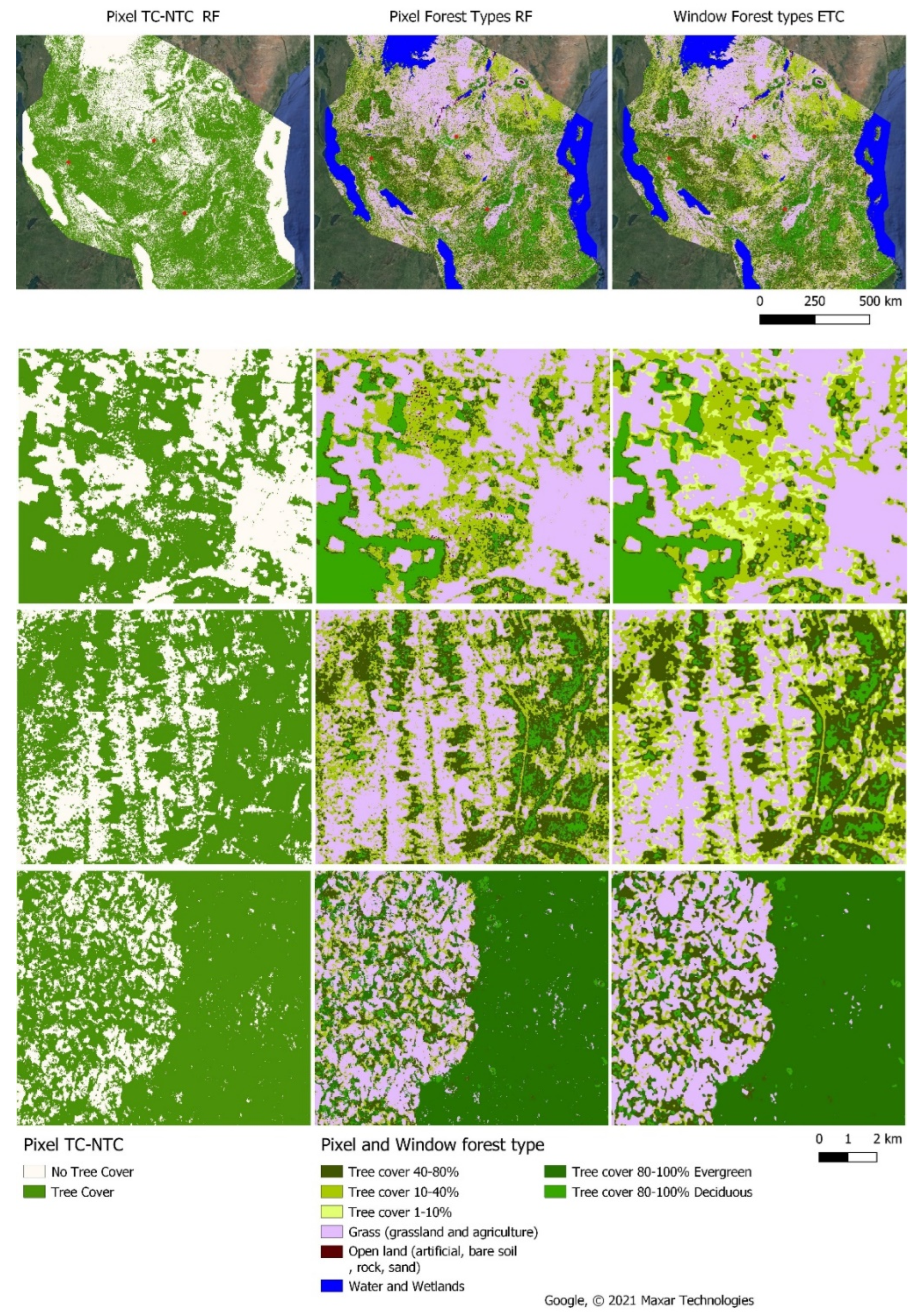
4.2. The Tree Cover–No Tree Cover and Forest Types Maps

The classification of a 10 m spatial resolution data source with ad-hoc training produced consistent maps showing the different categories of tree cover over Tanzania. We captured the spatial distribution of the tree cover in three different ways. As shown in Figure 9, the tree cover–no tree cover map gave an indication of where trees were present but it did not give information on the tree cover’s density. The two approaches (pixel and window) that mapped the different forest types offered a more detail picture of the spatial distribution of the canopy cover of the different forests in Tanzania. While the “window” approach presented a more “patchy” representation of the different classes than the “pixel” approach, it did give additional information about the presence of single trees in some of the pixels.

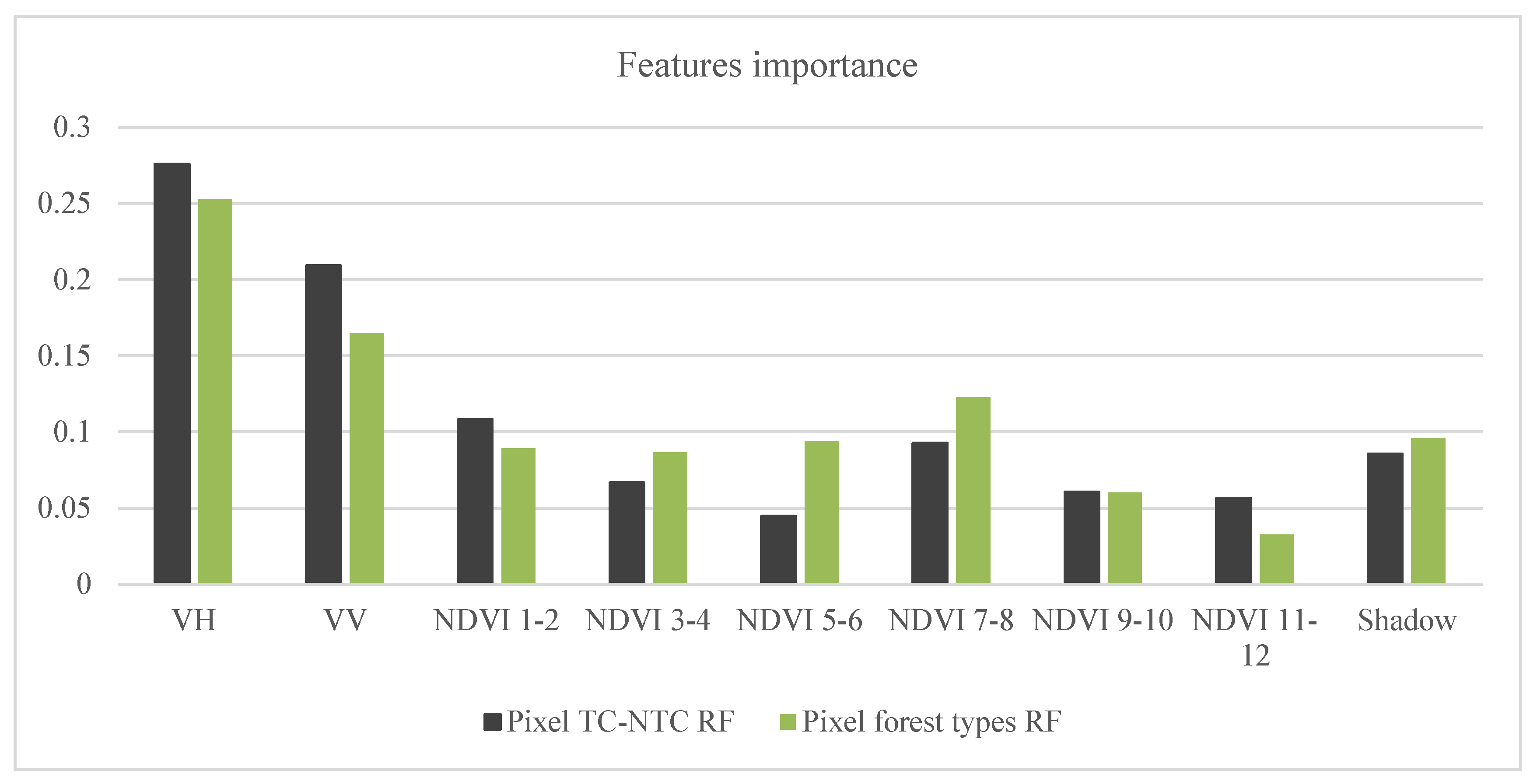
4.3. Features’ Importance

Both RF and ETC are capable of measuring a feature’s significance during the growing of the decision trees. In this application, the Gini index has been used to rank the spectral and temporal features. The Gini indices were analyzed in order to identify the influential spectral and temporal features. The two radar backscatters VV and VH were identified as the most important features, despite being annual composites (Figure 10).

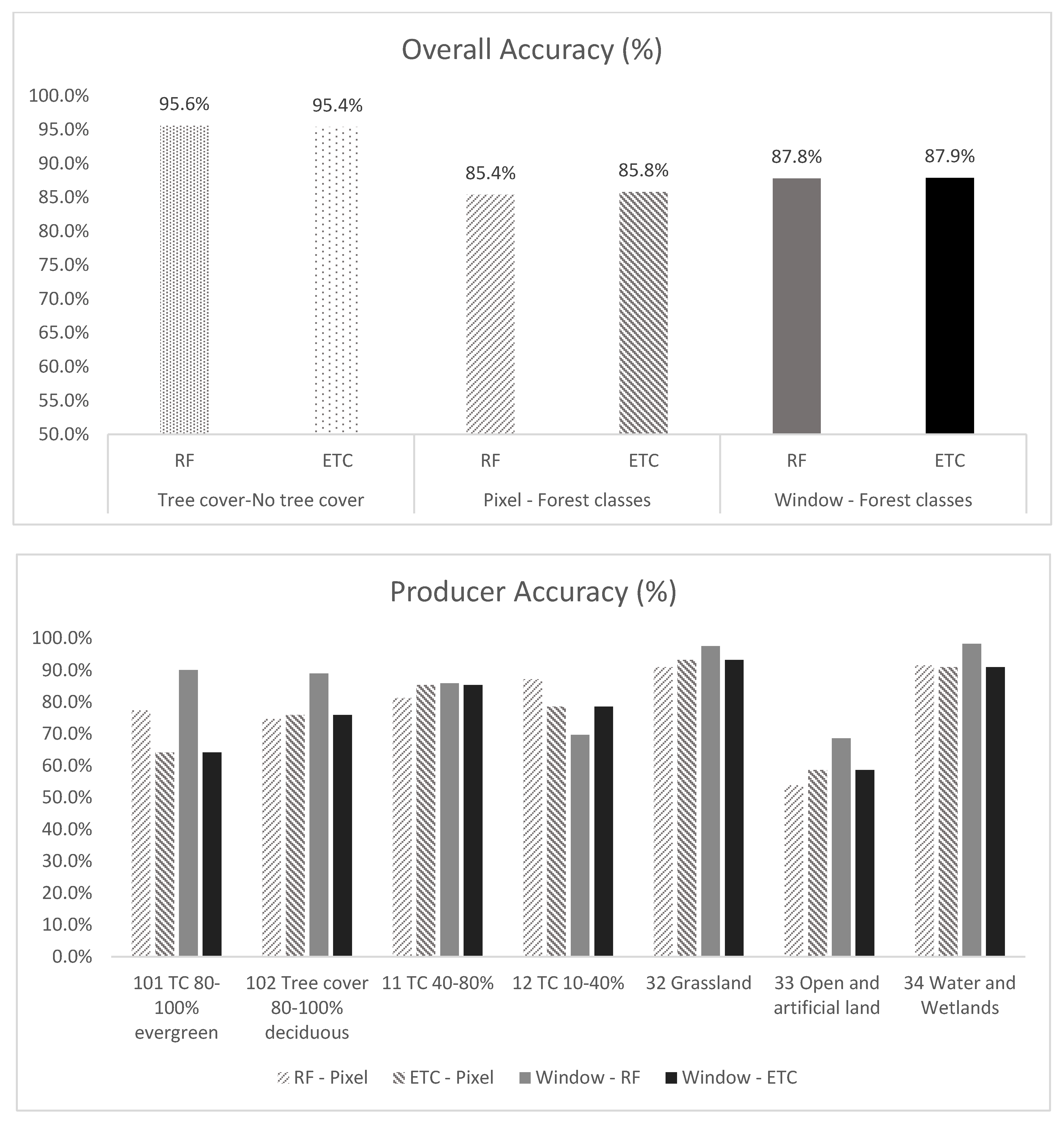
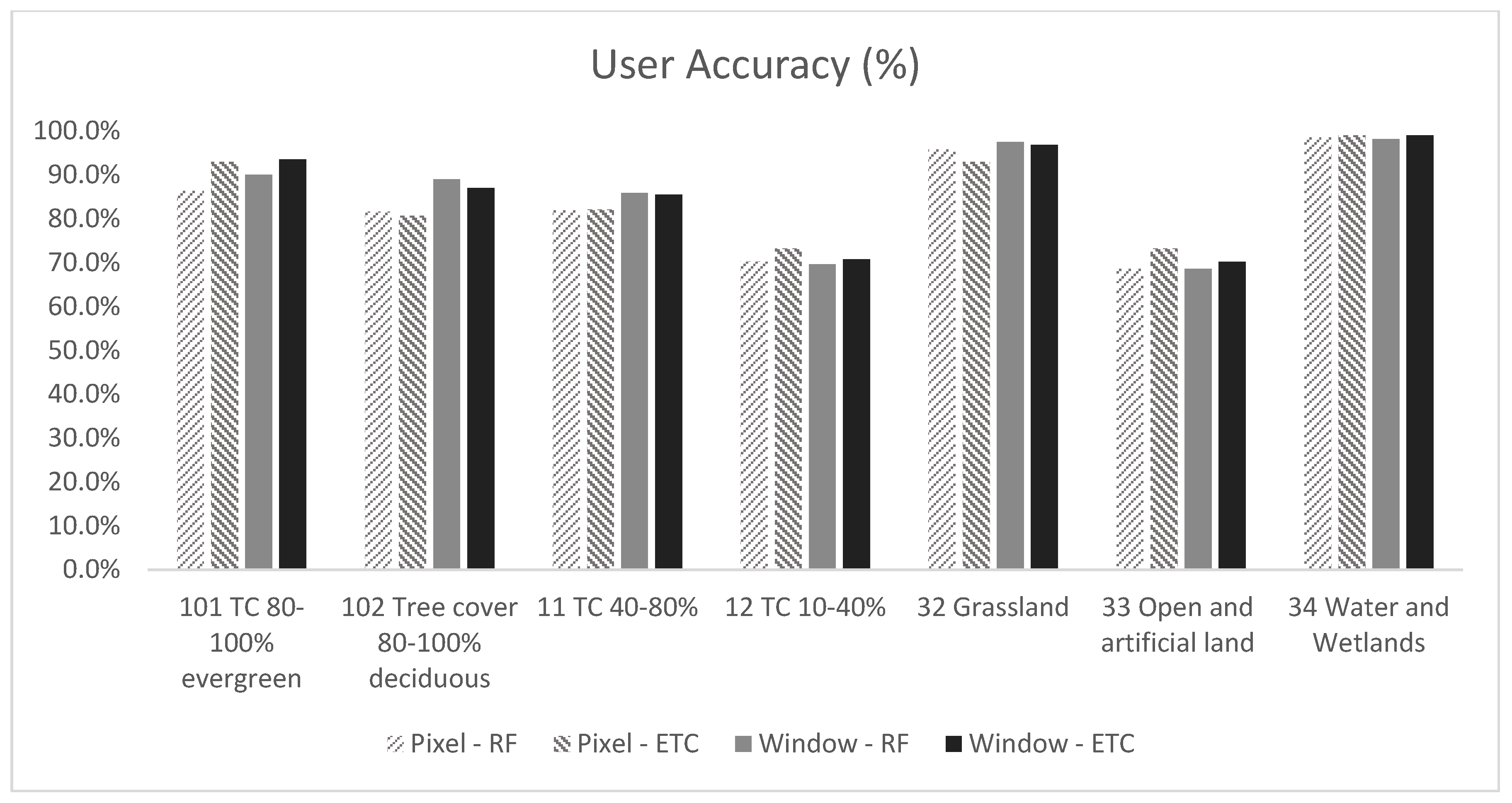
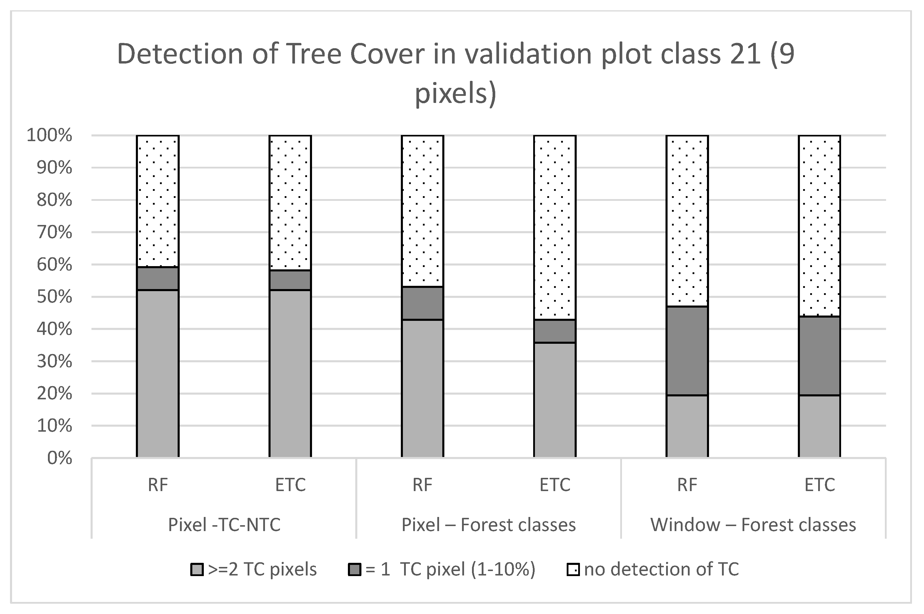
4.4. Accuracy Assessment

The different classification workflows were compared based on their accuracy metrics. Figure 11 reports the OA for the 6 maps that were obtained. The binary maps capturing only the presence and absence of tree cover have the highest accuracy, with an OA higher than 95%. For the classification representing the forest type, the “window” approach, wherein the spatial context is taken into account, outperformed the “pixel” approach in terms of OA (87% versus 85%). With respect to the OA, the difference between the RF and the ETC classifier was not important. When looking at the PA and UA, a greater difference between the two classifiers was visible, especially between the RF and ETC classifiers in regard to the “window” approach. Lower values of PA were observed for the ETC classifier with reference to the 80–100% forest classes indicating higher omission errors for those classes compared to RF.
The second part of the accuracy assessment evaluated the discrimination of single trees within the 98 samples that were labelled class 21 (Figure 12). We saw that the different models captured any type of tree cover class (including class 21) in about half of the samples that were identified as class 21 (Figure 13). The window classification model outperformed the other models, as it gave a more accurate representation of the tree cover percentage in those samples that were labelled as having a 1–10% tree cover. However, the analysis highlights that the discrimination of single trees is still a challenge when using satellite imagery at a 10 m spatial resolution.

4.5. Forest Cover Types’ Area Estimation

In Table 3, we derived the estimated area of forest cover types by pixel-counting and by deriving an area estimation from the error matrix [60] for one map for each classification workflow (RF for tree cover–no tree cover, RF for forest type “pixel” and ETC for forest type “window”). The area that was derived from the pixel-counting gives an estimation of the tree cover in the same area of magnitude for the three approaches, while the area estimation that was derived from the error matrix varies, with about 150,000 km2 of additional forest cover estimated in the “window” approach. That approach is the one which gives the most important estimate of tree cover in the country (when all classes of tree cover are considered).
The binary tree cover approach regroups all of the different forest types without discrimination (also visible in Figure 9). The two approaches which do discriminate the forest types give a more accurate indication of the different types of tree cover range. Comparing the two forest type approaches, we see that the “pixel” and the “window” approaches give stable estimations for the closer types of forest (tree cover > 40%) and vary more for the 10–40% class. The 1–10% class adds to the total area of land that is covered by tree cover.

5. Discussion

In order to map the tree cover and forest cover types over Tanzania, we have combined Copernicus S1 and S2 data with an ad-hoc reference training dataset and tested two different approaches that may be used to integrate the spatial information into classification algorithms. The combined use of S1 and S2 data allows us to produce maps of dry forests with an OA above 85% when capturing different forest cover types and above 95% for binary tree cover–no tree cover maps. The binary maps yielded higher accuracy but did not discriminate between the different forest types that present different biodiversity properties and carbon contents. Accurate information on forest type area improves the reporting of future carbon emission or gains to the UNFCCC in the framework of REDD+.
The launch of the Sentinel missions and their free data policy are changing the paradigm of satellite-based tropical forest monitoring [55]. Both the increased spatial and temporal resolutions of the S1 and S2 platforms are currently being explored and tested in order to tackle technical challenges such as seasonality and sparse tree cover in the tropical domain [19,61,62,63]. In tropical regions, the presence of clouds during most of the year is limiting the production of cloud-free composites, despite the 5 days revisiting time of combined S2A and S2B satellites [64]. In this study, we see that, despite the frequent cloud coverage, bi-monthly NDVI composites can be built with S2 over Tanzania. Being able to take into account the seasonality in classification algorithms improves the algorithms’ ability to discriminate between the different vegetation formations, as they lose their leaves and structure at different times. The importance of S1 is also highlighted in this specific study, calling for more integration of SAR data in dry forest monitoring [19,23].
However, the 10 m resolution still presents limitations for capturing Trees outside forests (TOF). TOF are an important natural resource that contributes to the carbon stock [65] and are usually underestimated in dry areas. The approach that was used in this study, taking into account a spatial window in order to better discriminate the class of 1–10% tree cover, allowed us to take into account a higher area that was covered by single trees than would have been possible with traditional approaches. However, many single trees are still missed. Approaches that automate the extraction of tree crowns from VHR images in dry environments show promising results for improving the counting of isolated trees in dry environments [66].
It is important to note that the maps that were used in this study do not distinguish open natural forest from degraded ones (e.g., landscapes from which tall trees have been removed). Forest degradation is a process of changes within the forest which negatively affect the structure or function of the stand or site and thereby lower its capacity to supply products or services [67]. An exhaustive assessment of past degradation would need to be based on a long-time series of satellite imagery, such as that which has been conducted in moist tropical forests [6]. Methods targeting the monitoring of forest degradation and forest disturbances [19,68] could be used in combination with the forest cover maps that have been presented in this study in order to assess and map the forest degradation that has happened in the following years (i.e., post 2018).
The advances in dry tropical forest mapping that are demonstrated in this study can be integrated into national monitoring systems. Open data from Copernicus were used in combination with publicly available tools such as Collect Earth and the Google Earth Engine platform.
A unique expert-based training dataset that is suitable to dry forest monitoring applications with EO data was created for this specific study and is available to be re-used for other studies. The reference dataset of 4196 samples was created by the visual interpretation of VHR images on a spatial window of 0.25 ha. The spatial window allowed the capture of the canopy cover of the different forest classes. The reference dataset that was created is a multi-level legend and was used at different levels of complexity.
The archive of satellite data that were made available in recent years represents an amount of data that cannot be handled with traditional techniques. The challenges of classifying the annual time series of EO data are commonly tackled by machine learning approaches while keeping a place for user interaction. Such algorithms require input layers that are prepared and selected accordingly. The user interaction takes place in the selection of those layers and the construction of the ad-hoc training and validation dataset. More advanced users can test the fitness of different algorithms to their mapping requirements. In the context of NFMS, national institutions favor flexible approaches that they can have full control over [29]. The methodology that was followed here can be easily adopted at different levels of complexity while ensuring a timely production of maps in the Eastern African region. From a capacity development perspective, such a study could lead to the development of toolkits for (i) facilitating the access to pre-processed S1 and S2 data time series (ii) producing meaningful layers for dry forest mapping and monitoring and (iii) allowing the incorporation of available national or local training datasets.

6. Conclusions

This study demonstrates that S1 and S2 imagery is well suited for forest monitoring in East Africa. We have illustrated that different automated classification approaches can be used to address different thematic needs. While pixel-based classification approaches are an appropriate fit for a tree cover–no tree cover task, considering neighboring pixels allows one to take more information from the spatial context into account, including a better discrimination of the trees that are outside the forest in landcover maps.
Following the methodology that was presented in this study, recent forest maps with high accuracy can be created at a national scale and be used as a baseline for forest cover change monitoring.
The three-fold combination of machine learning, the adequate processing of S1 and S2 data for dry forest monitoring and a custom-made reference dataset is a replicable methodology that can be potentially applied to other Eastern African countries in the context of national monitoring services.

Author Contributions

Conceptualization, A.V., K.K. and H.E.; methodology, A.V., K.K. and V.S.; validation, A.V., K.K. and H.E.; formal analysis, A.V., K.K. and V.S.; investigation, A.V., K.K. and V.S.; data curation, A.V.; writing—original draft preparation, A.V., K.K. and H.E.; writing—review and editing, A.V., V.S., H.E. and F.A.; visualization, A.V. and K.K.; supervision, A.V., H.E. and F.A.; project administration, H.E. and F.A. All authors have read and agreed to the published version of the manuscript.

Funding

This research received no external funding.

Institutional Review Board Statement

Not applicable.

Data Availability Statement

The code that was used to generate the S1 and S2 mosaics, the expert-based reference dataset and the three best maps from each classification workflow are available for download here https://doi.org/10.1594/PANGAEA.940264 (accessed on 1 January 2022). The folder “reference_dataset.zip” contains the expert-based training and validation dataset. The point shapefile that corresponds to the center of the plot, as well as the 3 × 3 and 5 × 5 polygon shapefile, are shared together with a qml layer file for each type of shapefile. Three maps (binary TC-NTC “pixel” RF, forest type “pixel” RF and “window” ETC) are also shared. A 40 km buffer from national boundaries is kept in order to let users refine their area of interest. The qml style files are also shared. In the “script.zip” folder, the JavaScript codes that are required in order to generate the S1 and S2 mosaics are shared.

Acknowledgments

The authors thank Bruno Combal for sharing his work related to forest monitoring in East Africa and Silvia Carboni for her help with the reference dataset’s design and the visual interpretation of the reference data.

Conflicts of Interest

The authors declare no conflict of interest.

References

  1. Sandker, M.; Carrillo, O.; Leng, C.; Lee, D.; D’Annunzio, R.; Fox, J. The Importance of High–Quality Data for REDD+ Monitoring and Reporting. Forests 2021, 12, 99. [Google Scholar] [CrossRef]
  2. Morales-Hidalgo, D.; Kleinn, C.; Scott, C.T. Voluntary Guidelines on National Forest Monitoring; FAO, Ed.; Food and Agriculture Organization of the United Nations: Rome, Italy, 2017; ISBN 978-92-5-109619-2. [Google Scholar]
  3. Nesha, M.K.; Herold, M.; De Sy, V.; Duchelle, A.E.; Martius, C.; Branthomme, A.; Garzuglia, M.; Jonsson, O.; Pekkarinen, A. An assessment of data sources, data quality and changes in national forest monitoring capacities in the Global Forest Resources Assessment 2005–2020. Environ. Res. Lett. 2021, 16, 054029. [Google Scholar] [CrossRef]
  4. UNFCCC National Forest Monitoring System. Available online: https://redd.unfccc.int/fact-sheets/national-forest-monitoring-system.html (accessed on 9 January 2021).
  5. Hansen, M.C.; Potapov, P.V.; Moore, R.; Hancher, M.; Turubanova, S.A.; Tyukavina, A.; Thau, D.; Stehman, S.V.; Goetz, S.J.; Loveland, T.R.; et al. High-Resolution Global Maps of 21st-Century Forest Cover Change. Science 2013, 342, 850–853. [Google Scholar] [CrossRef] [PubMed] [Green Version]
  6. Vancutsem, C.; Achard, F.; Pekel, J.-F.; Vieilledent, G.; Carboni, S.; Simonetti, D.; Gallego, J.; Aragão, L.E.O.C.; Nasi, R. Long-term (1990–2019) monitoring of forest cover changes in the humid tropics. Sci. Adv. 2021, 7, eabe1603. [Google Scholar] [CrossRef] [PubMed]
  7. Kim, D.-H.; Sexton, J.O.; Noojipady, P.; Huang, C.; Anand, A.; Channan, S.; Feng, M.; Townshend, J.R. Global, Landsat-based forest-cover change from 1990 to 2000. Remote Sens. Environ. 2014, 155, 178–193. [Google Scholar] [CrossRef] [Green Version]
  8. Badjana, H.M.; Olofsson, P.; Woodcock, C.E.; Helmschrot, J.; Wala, K.; Akpagana, K. Mapping and estimating land change between 2001 and 2013 in a heterogeneous landscape in West Africa: Loss of forestlands and capacity building opportunities. Int. J. Appl. Earth Obs. Geoinf. 2017, 63, 15–23. [Google Scholar] [CrossRef]
  9. Bouvet, A.; Mermoz, S.; Le Toan, T.; Villard, L.; Mathieu, R.; Naidoo, L.; Asner, G.P. An above-ground biomass map of African savannahs and woodlands at 25 m resolution derived from ALOS PALSAR. Remote Sens. Environ. 2018, 206, 156–173. [Google Scholar] [CrossRef]
  10. Bastin, J.-F.; Berrahmouni, N.; Grainger, A.; Maniatis, D.; Mollicone, D.; Moore, R.; Patriarca, C.; Picard, N.; Sparrow, B.; Abraham, E.M.; et al. The extent of forest in dryland biomes. Science 2017, 356, 635–638. [Google Scholar] [CrossRef] [Green Version]
  11. INPE Projeto Prodes—Monitoramento Da Floresta Amazônica Brasileira Por Satélite. Available online: http://www.obt.inpe.br/OBT/assuntos/programas/amazonia/prodes (accessed on 12 June 2020).
  12. Achard, F.; Eva, H.D.; Mayaux, P.; Stibig, H.-J.; Belward, A. Improved estimates of net carbon emissions from land cover change in the tropics for the 1990s. Global Biogeochem. Cycles 2004, 18, GB2008. [Google Scholar] [CrossRef]
  13. Næsset, E.; Ørka, H.O.; Solberg, S.; Bollands\aas, O.M.; Hansen, E.H.; Mauya, E.; Zahabu, E.; Malimbwi, R.; Chamuya, N.; Olsson, H.; et al. Mapping and estimating forest area and aboveground biomass in miombo woodlands in Tanzania using data from airborne laser scanning, TanDEM-X, RapidEye, and global forest maps: A comparison of estimated precision. Remote Sens. Environ. 2016, 175, 282–300. [Google Scholar] [CrossRef]
  14. Baumann, M.; Levers, C.; Macchi, L.; Bluhm, H.; Waske, B.; Gasparri, N.I.; Kuemmerle, T. Mapping continuous fields of tree and shrub cover across the Gran Chaco using Landsat 8 and Sentinel-1 data. Remote Sens. Environ. 2018, 216, 201–211. [Google Scholar] [CrossRef]
  15. Timberlake, J.; Chidumayo, E.; Sawadogo, L. Distribution and Characteristics of African Dry Forests and Woodlands. In The Dry Forests and Woodlands of Africa: Managing for Products and Services; Earthscan: London, UK; Washington, DC, USA, 2010; ISBN 978-1-84977-654-7. [Google Scholar]
  16. Furley, P.A. Tropical savannas and associated forests: Vegetation and plant ecology. Prog. Phys. Geogr. Earth Environ. 2007, 31, 203–211. [Google Scholar] [CrossRef]
  17. FAO. Trees, Forests and Land Use in Drylands: The First Global Assessment; Food and Agriculture Organization of the United Nations: Rome, Italy, 2019; ISBN iSBN9789251093269. [Google Scholar]
  18. Reiche, J.; Hamunyela, E.; Verbesselt, J.; Hoekman, D.; Herold, M. Improving near-real time deforestation monitoring in tropical dry forests by combining dense Sentinel-1 time series with Landsat and ALOS-2 PALSAR-2. Remote Sens. Environ. 2018, 204, 147–161. [Google Scholar] [CrossRef]
  19. Reiche, J.; Mullissa, A.; Slagter, B.; Gou, Y.; Tsendbazar, N.E.; Odongo-Braun, C.; Vollrath, A.; Weisse, M.J.; Stolle, F.; Pickens, A.; et al. Forest disturbance alerts for the Congo Basin using Sentinel-1. Environ. Res. Lett. 2021, 16. [Google Scholar] [CrossRef]
  20. Hojas-Gascón, L.; Belward, A.; Eva, H.; Ceccherini, G.; Hagolle, O.; Garcia, J.; Cerutti, P. Potential improvement for forest cover and forest degradation mapping with the forthcoming Sentinel-2 program. Int. Arch. Photogramm. Remote Sens. Spat. Inf. Sci.-ISPRS Arch. 2015, 40, 417–423. [Google Scholar] [CrossRef] [Green Version]
  21. Anchang, J.Y.; Prihodko, L.; Ji, W.; Kumar, S.S.; Ross, C.W.; Yu, Q.; Lind, B.; Sarr, M.A.; Diouf, A.A.; Hanan, N.P. Toward Operational Mapping of Woody Canopy Cover in Tropical Savannas Using Google Earth Engine. Front. Environ. Sci. 2020, 8, 4. [Google Scholar] [CrossRef] [Green Version]
  22. Lopes, M.; Frison, P.L.; Durant, S.M.; Schulte to Bühne, H.; Ipavec, A.; Lapeyre, V.; Pettorelli, N. Combining optical and radar satellite image time series to map natural vegetation: Savannas as an example. Remote Sens. Ecol. Conserv. 2020, 6, 316–326. [Google Scholar] [CrossRef]
  23. Zhang, W.; Brandt, M.; Wang, Q.; Prishchepov, A.V.; Tucker, C.J.; Li, Y.; Lyu, H.; Fensholt, R. From woody cover to woody canopies: How Sentinel-1 and Sentinel-2 data advance the mapping of woody plants in savannas. Remote Sens. Environ. 2019, 234, 111465. [Google Scholar] [CrossRef]
  24. Shimizu, K.; Ota, T.; Mizoue, N. Detecting Forest Changes Using Dense Landsat 8 and Sentinel-1 Time Series Data in Tropical Seasonal Forests. Remote Sens. 2019, 11, 1899. [Google Scholar] [CrossRef] [Green Version]
  25. Heckel, K.; Urban, M.; Schratz, P.; Mahecha, M.; Schmullius, C. Predicting Forest Cover in Distinct Ecosystems: The Potential of Multi-Source Sentinel-1 and -2 Data Fusion. Remote Sens. 2020, 12, 302. [Google Scholar] [CrossRef] [Green Version]
  26. Gorelick, N.; Hancher, M.; Dixon, M.; Ilyushchenko, S.; Thau, D.; Moore, R. Google Earth Engine: Planetary-scale geospatial analysis for everyone. Remote Sens. Environ. 2017, 202, 18–27. [Google Scholar] [CrossRef]
  27. Bey, A.; Jetimane, J.; Lisboa, S.N.; Ribeiro, N.; Sitoe, A.; Meyfroidt, P. Mapping smallholder and large-scale cropland dynamics with a flexible classification system and pixel-based composites in an emerging frontier of Mozambique. Remote Sens. Environ. 2020, 239, 111611. [Google Scholar] [CrossRef]
  28. Lopes, C.; Leite, A.; Vasconcelos, M.J. Open-access cloud resources contribute to mainstream REDD+: The case of Mozambique. Land Use Policy 2019, 82, 48–60. [Google Scholar] [CrossRef]
  29. Saah, D.; Tenneson, K.; Matin, M.; Uddin, K.; Cutter, P.; Poortinga, A.; Nguyen, Q.H.; Patterson, M.; Johnson, G.; Markert, K.; et al. Land Cover Mapping in Data Scarce Environments: Challenges and Opportunities. Front. Environ. Sci. 2019, 7, 150. [Google Scholar] [CrossRef] [Green Version]
  30. Saah, D.; Tenneson, K.; Poortinga, A.; Nguyen, Q.; Chishtie, F.; Aung, K.S.; Markert, K.N.; Clinton, N.; Anderson, E.R.; Cutter, P.; et al. Primitives as building blocks for constructing land cover maps. Int. J. Appl. Earth Obs. Geoinf. 2020, 85, 101979. [Google Scholar] [CrossRef]
  31. McSweeney, C.; New, M.; Lizcano, G. UNDP Climate Change Country Profiles: Tanzania. Available online: https://digital.library.unt.edu/ark:/67531/metadc226754/ (accessed on 1 December 2021).
  32. MWE. Tanzania Second National Communication to the United Nations Framework Convention on Climate Change; Division of Environment Tanzania: Dar es Salaam, Tanzania, 2014. [Google Scholar]
  33. Felix, M.; Gheewala, S.H. Review of Biomass Energy Dependency in Tanzania. Energy Procedia 2011, 9, 338–343. [Google Scholar] [CrossRef] [Green Version]
  34. Lovett, J.C. Moist forests of Tanzania. Swara 1985, 8, 8–9. [Google Scholar]
  35. Burgess, N.D.; Clarke, G.P.; Rodgers, W.A. Coastal forests of eastern Africa: Status, endemism patterns and their potential causes. Biol. J. Linn. Soc. 1998, 64, 337–367. [Google Scholar] [CrossRef]
  36. Isango, J. Stand Structure and Tree Species Composition of Tanzania Miombo Woodlands: A Case Study from Miombo Woodlands of Community Based Forest Management in Iringa District; Working Papers of the Finnish Forest Research Institute. In Proceedings of the 1st MITIMIOMBO Project Workshop, Morogoro, Tanzania, 6–12 February 2007; Volume 50, pp. 43–56. [Google Scholar]
  37. FAO. Global Forest Resources Assessment 2015; Food and Agriculture Organization of the United Nations: Rome, Italy, 2015. [Google Scholar]
  38. Drusch, M.; Del Bello, U.; Carlier, S.; Colin, O.; Fernandez, V.; Gascon, F.; Hoersch, B.; Isola, C.; Laberinti, P.; Martimort, P.; et al. Sentinel-2: ESA’s Optical High-Resolution Mission for GMES Operational Services. Remote Sens. Environ. 2012, 120, 25–36. [Google Scholar] [CrossRef]
  39. Song, C.; Woodcock, C.E.; Seto, K.C.; Lenney, M.P.; Macomber, S.A. Classification and Change Detection Using Landsat TM Data: When and How to Correct Atmospheric Effects? Remote Sens. Environ. 2001, 75, 230–244. [Google Scholar] [CrossRef]
  40. Housman, I.W.; Chastain, R.A.; Finco, M.V. An evaluation of forest health insect and disease survey data and satellite-based remote sensing forest change detection methods: Case studies in the United States. Remote Sens. 2018, 10, 1184. [Google Scholar] [CrossRef] [Green Version]
  41. Meroni, M.; D’Andrimont, R.; Vrieling, A.; Fasbender, D.; Lemoine, G.; Rembold, F.; Seguini, L.; Verhegghen, A. Comparing land surface phenology of major European crops as derived from SAR and multispectral data of Sentinel-1 and -2. Remote Sens. Environ. 2021, 253, 112232. [Google Scholar] [CrossRef] [PubMed]
  42. Gao, B. NDWI–A normalized difference water index for remote sensing of vegetation liquid water from space. Remote Sens. Environ. 1996, 58, 257–266. [Google Scholar] [CrossRef]
  43. Rikimaru, A.; Roy, P.S.; Miyatake, S. Tropical forest cover density mapping. Trop. Ecol. 2002, 43, 39–47. [Google Scholar]
  44. Tucker, C.J. Red and photographic infrared linear combinations for monitoring vegetation. Remote Sens. Environ. 1979, 8, 127–150. [Google Scholar] [CrossRef] [Green Version]
  45. Hojas Gascón, L.; Ceccherini, G.; García Haro, F.; Avitabile, V.; Eva, H. The Potential of High Resolution (5 m) RapidEye Optical Data to Estimate Above Ground Biomass at the National Level over Tanzania. Forests 2019, 10, 107. [Google Scholar] [CrossRef] [Green Version]
  46. Torres, R.; Snoeij, P.; Geudtner, D.; Bibby, D.; Davidson, M.; Attema, E.; Potin, P.; Rommen, B.; Floury, N.; Brown, M.; et al. GMES Sentinel-1 mission. Remote Sens. Environ. 2012, 120, 9–24. [Google Scholar] [CrossRef]
  47. ESA Sentinel-1 SAR User Guide. Available online: https://sentinel.esa.int/web/sentinel/user-guides/sentinel-1-sar (accessed on 21 September 2021).
  48. ESA The Sentinel-1 Toolbox—Version 7. Available online: https://sentinels.copernicus.eu/web/sentinel/866toolboxes/sentinel-1 (accessed on 21 September 2021).
  49. Frison, P.L.; Fruneau, B.; Kmiha, S.; Soudani, K.; Dufrêne, E.; Le Toan, T.; Koleck, T.; Villard, L.; Mougin, E.; Rudant, J.P. Potential of Sentinel-1 data for monitoring temperate mixed forest phenology. Remote Sens. 2018, 10, 2049. [Google Scholar] [CrossRef] [Green Version]
  50. Rüetschi, M.; Schaepman, M.E.; Small, D. Using Multitemporal Sentinel-1 C-band Backscatter to Monitor Phenology and Classify Deciduous and Coniferous Forests in Northern Switzerland. Remote Sens. 2017, 10, 55. [Google Scholar] [CrossRef] [Green Version]
  51. MNRT. National Forest Resources Monitoring and Assessment of Tanzania Mainland (NAFORMA); Main results; Ministry of Natural Resources and Tourism, Tanzania Forest Services Agency: Dar es Salaam, Tanzania, 2015.
  52. Mauya, E.W.; Mugasha, W.A.; Njana, M.A.; Zahabu, E.; Malimbwi, R. Carbon stocks for different land cover types in Mainland Tanzania. Carbon Balance Manag. 2019, 14, 4. [Google Scholar] [CrossRef] [Green Version]
  53. FAO. Map Accuracy Assessment and Area Estimation Map Accuracy Assessment and Area Estimation: A Practical Guide. In National Forest Monitoring Assessment Working Paper; Food and Agriculture Organization of the United Nations: Rome, Italy, 2016; p. 69. [Google Scholar]
  54. Bey, A.; Sánchez-Paus Díaz, A.; Maniatis, D.; Marchi, G.; Mollicone, D.; Ricci, S.; Bastin, J.-F.; Moore, R.; Federici, S.; Rezende, M.; et al. Collect Earth: Land Use and Land Cover Assessment through Augmented Visual Interpretation. Remote Sens. 2016, 8, 807. [Google Scholar] [CrossRef] [Green Version]
  55. Schepaschenko, D.; See, L.; Lesiv, M.; Bastin, J.-F.; Mollicone, D.; Tsendbazar, N.-E.; Bastin, L.; McCallum, I.; Laso Bayas, J.C.; Baklanov, A.; et al. Recent Advances in Forest Observation with Visual Interpretation of Very High-Resolution Imagery. Surv. Geophys. 2019, 40, 839–862. [Google Scholar] [CrossRef] [Green Version]
  56. Soille, P.; Burger, A.; De Marchi, D.; Kempeneers, P.; Rodriguez, D.; Syrris, V.; Vasilev, V. A versatile data-intensive computing platform for information retrieval from big geospatial data. Future Gener. Comput. Syst. 2018, 81, 30–40. [Google Scholar] [CrossRef]
  57. Pedregosa, F.; Varoquaux, G.; Gramfort, A.; Michel, V.; Thirion, B.; Grisel, O.; Blondel, M.; Prettenhofer, P.; Weiss, R.; Dubourg, V.; et al. Scikit-learn: Machine Learning in Python. J. Mach. Learn. Res. 2011, 12, 2825–2830. [Google Scholar]
  58. Stehman, S.V.; Czaplewski, R.L. Design and analysis for thematic map accuracy assessment: Fundamental principles. Remote Sens. Environ. 1998, 64, 331–344. [Google Scholar] [CrossRef]
  59. Stehman, S.V.; Wickham, J.D. Pixels, blocks of pixels, and polygons: Choosing a spatial unit for thematic accuracy assessment. Remote Sens. Environ. 2011, 115, 3044–3055. [Google Scholar] [CrossRef]
  60. Olofsson, P.; Foody, G.M.; Herold, M.; Stehman, S.V.; Woodcock, C.E.; Wulder, M.A. Good practices for estimating area and assessing accuracy of land change. Remote Sens. Environ. 2014, 148, 42–57. [Google Scholar] [CrossRef]
  61. Zhang, Y.; Ling, F.; Wang, X.; Foody, G.M.; Boyd, D.S.; Li, X.; Du, Y.; Atkinson, P.M. Tracking small-scale tropical forest disturbances: Fusing the Landsat and Sentinel-2 data record. Remote Sens. Environ. 2021, 261, 112470. [Google Scholar] [CrossRef]
  62. Lima, T.A. Comparing Sentinel-2 MSI and Landsat 8 OLI Imagery for Monitoring Selective Logging in the Brazilian Amazon. Remote Sens. 2019, 8, 961. [Google Scholar] [CrossRef] [Green Version]
  63. Verhegghen, A.; Eva, H.; Ceccherini, G.; Achard, F.; Gond, V.; Gourlet-Fleury, S.; Cerutti, P. The Potential of Sentinel Satellites for Burnt Area Mapping and Monitoring in the Congo Basin Forests. Remote Sens. 2016, 8, 986. [Google Scholar] [CrossRef] [Green Version]
  64. Simonetti, D.; Pimple, U.; Langner, A.; Marelli, A. Pan-Tropical Sentinel-2 Cloud-Free Annual Composite. Data Brief 2021, 39, 107488. [Google Scholar] [CrossRef] [PubMed]
  65. Schnell, S.; Kleinn, C.; Ståhl, G. Monitoring trees outside forests: A review. Environ. Monit. Assess. 2015, 187, 600. [Google Scholar] [CrossRef] [PubMed]
  66. Brandt, M.; Tucker, C.J.; Kariryaa, A.; Rasmussen, K.; Abel, C.; Small, J.; Chave, J.; Rasmussen, L.V.; Hiernaux, P.; Diouf, A.A.; et al. An unexpectedly large count of trees in the West African Sahara and Sahel. Nature 2020, 587, 78–82. [Google Scholar] [CrossRef] [PubMed]
  67. FAO. Assessing forest degradation—Towards the development of globally applicable guidelines. In Forest Resources Assessment Working Paper 117; Food and Agriculture Organization of the United Nations: Rome, Italy, 2011. [Google Scholar]
  68. Langner, A.; Miettinen, J.; Kukkonen, M.; Vancutsem, C.; Simonetti, D.; Vieilledent, G.; Verhegghen, A.; Gallego, J.; Stibig, H.J. Towards operational monitoring of forest canopy disturbance in evergreen rain forests: A test case in continental Southeast Asia. Remote Sens. 2018, 10, 544. [Google Scholar] [CrossRef] [Green Version]
Figure 1. Challenges of tropical dry forests monitoring (A) Deciduous vegetation—same forest area in the humid (May) and the dry (July) season, (B) Fires—same forest area affected (2010) or not (2011) by fire, (C) Four different areas illustrating the variety of tree cover. “Maps data: Google, © 2021 Maxar Technologies”.
Remotesensing 14 01522 g001
Figure 2. Workflow diagram of the main methodological steps.
Remotesensing 14 01522 g002
Figure 3. NDVI bi-monthly compositing—number of cloud free observations.
Remotesensing 14 01522 g003
Figure 4. Example of temporal profiles (in Db) for the year 2018 in VV and VH polarization for different land cover classes.
Remotesensing 14 01522 g004
Figure 5. The 50 m by 50 m square plot interpreted in Collect Earth and the interpretation rules. Maps data: Google, © 2021 Maxar Technologies.
Remotesensing 14 01522 g005
Figure 6. Spatial distribution and number of samples of the reference dataset. Maps data: Google, © 2021 Maxar Technologies.
Remotesensing 14 01522 g006
Figure 7. “pixel” and “window” classification workflows.
Remotesensing 14 01522 g007
Figure 8. NDVI bi-monthly composites for 2018. The NDVI values from −1 to 1 are rescaled to 0–200.
Remotesensing 14 01522 g008
Figure 9. Resulting maps from the three classification workflows.
Remotesensing 14 01522 g009
Figure 10. Features’ importance for two classifications in the “pixel” approach.
Remotesensing 14 01522 g010
Figure 11. Overall accuracy, producer accuracy and user accuracy of the six maps based on the area proportion.
Remotesensing 14 01522 g011aRemotesensing 14 01522 g011b
Figure 12. Illustration of the class 21 1–10% tree cover for (a) the window–forest type classes ETC, (b) the pixel–forest type classes RF and (c) recent VHR images in Google Earth.
Remotesensing 14 01522 g012
Figure 13. Assessment of the class 1–10% tree cover for the 98 validation plots with a class 21.
Remotesensing 14 01522 g013
Table 1. The Sentinel-1 and Sentinel-2 layers selected for the classifications.
Satellite ConstellationIndex Temporal Interval Compositing Technique
Sentinel-2NDVIBi-monthly (6 layers)Maximum
Sentinel-2Shadow IndexAnnualMaximum of monthly 90th percentile
Sentinel-1VVAnnualMinimum of monthly 10th percentile
Sentinel-1VHAnnualMinimum of monthly 10th percentile
Table 2. Legend for the reference dataset.
Level 0Level 1Level 2
1Tree Cover ≥ 10% 1080–100% tree canopy closure 101Evergreen or semi-evergreen
102Deciduous
1140–80% tree canopy closure
1210–40% tree canopy closure
2Tree Cover 1–10%21Grass and “singles trees”
3No Tree Cover32Grass and/or agriculture
33Open land (artificial, bare soil, rock, sand)
34Water/wetlands
Table 3. Area estimation of the tree cover and forest types in Tanzania in the year 2018 for three different classification approaches.
Forest TypeTree Cover–No Tree Cover
Pixel Window Pixel
Area (km2)Area
Estimated
(km2)
95%
CI
Area (km2)Area
Estimated
(km2)
95%
CI
Area (km2)Area
Estimated
(km2)
95%
CI
Tree cover 80–100% evergreen10124,69927,5991661 21,29126,0491502
Tree cover 80–100% deciduous10298,517107,6783889 99,560100,3352957
Tree cover 40–80%11248,271250,108 5959248,529243,5595098
Tree cover 10–40%12190,722153,638 5472178,737266,1814950
Tree cover 1–10%21---24,09886,3575175
Tree cover 562,209539,023 572,215 722,482 587,980 558,7274052
Grassland32325,985342,9824408316,811285,6965248
Open and artificial land33578273641373470562391203
Water and wetlands3459,51664,122158459,72863,2991267
No tree cover 391,283414,469 381,244355,234 365,479 394,7324052
Publisher’s Note: MDPI stays neutral with regard to jurisdictional claims in published maps and institutional affiliations.

