Abstract
Scene classification is an active research area in the remote sensing (RS) domain. Some categories of RS scenes, such as medium residential and dense residential scenes, would contain the same type of geographical objects but have various spatial distributions among these objects. The adjacency and disjointness relationships among geographical objects are normally neglected by existing RS scene classification methods using convolutional neural networks (CNNs). In this study, a multi-output network (MopNet) combining a graph neural network (GNN) and a CNN is proposed for RS scene classification with a joint loss. In a candidate RS image for scene classification, superpixel regions are constructed through image segmentation and are represented as graph nodes, while graph edges between nodes are created according to the spatial adjacency among corresponding superpixel regions. A training strategy of a jointly learning CNN and GNN is adopted in the MopNet. Through the message propagation mechanism of MopNet, spatial and topological relationships imbedded in the edges of graphs are employed. The parameters of the CNN and GNN in MopNet are updated simultaneously with the guidance of a joint loss via the backpropagation mechanism. Experimental results on the OPTIMAL-31 and aerial image dataset (AID) datasets show that the proposed MopNet combining a graph convolutional network (GCN) or graph attention network (GAT) and ResNet50 achieves state-of-the-art accuracy. The overall accuracy obtained on OPTIMAL-31 is 96.06% and those on AID are 95.53% and 97.11% under training ratios of 20% and 50%, respectively. Spatial and topological relationships imbedded in RS images are helpful for improving the performance of scene classification.
1. Introduction
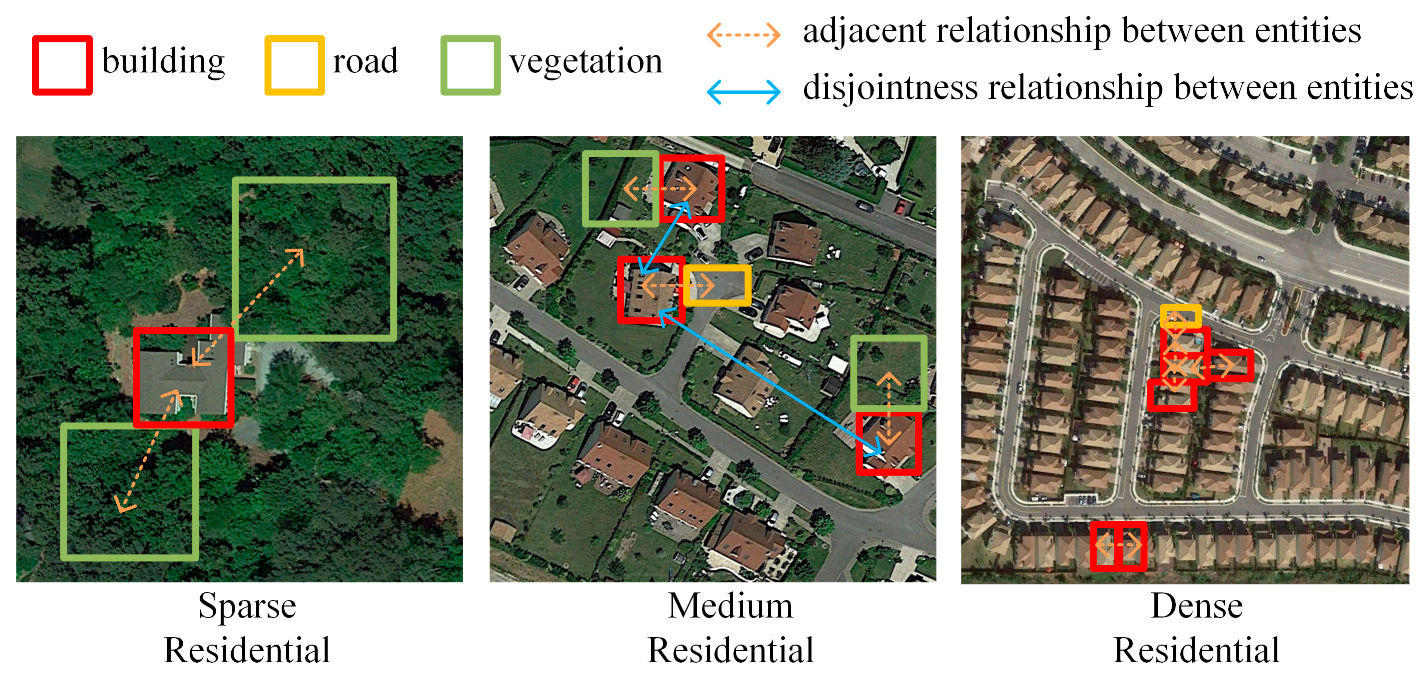
Remote sensing (RS) image scene classification is an active research area essential for image understanding at the scene level [1]. RS image scene classification focuses on categorizing images using semantic information. The task of RS image scene classification aims to discriminate images of various categories in an image dataset, giving one label to each scene image [1]. Scene classification is different from image segmentation or object-oriented classification, giving one label to each pixel or object. The spatial and topological relationships imbedded in RS images are invariant to image transformation, such as panning, distortion, or rotation, and are valuable for discriminating various categories of RS scenes. The adjacency and the disjointness relationships between objects are two types of commonly used spatial and topological dependency [2]. Some RS scene images contain the same type of geographical entities but have various spatial distributions among these entities and thus have different scene semantic labels. As shown in Figure 1, sparse residential, medium residential, and dense residential scenes consist of buildings, roads, and vegetation but have various adjacency or disjointness relationships among the entities.
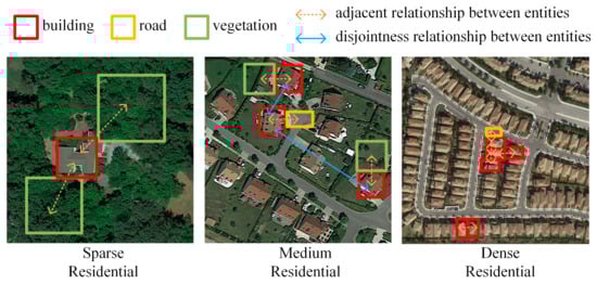
Figure 1.
Illustration of spatial and topological dependency among entities in RS scene images.
Existing methods of RS image scene classification usually neglect or do not exploit the spatial and topological relationships well. In earlier studies, handcrafted features, such as the color, texture, or bag-of-visual words, were widely applied in methods of RS image scene classification [3,4]. Handcrafted features typically require sufficient expert information to be designed or extracted and are not robust enough to various application scenarios [1]. Handcrafted features are usually inadequate in representing high-level semantics of RS images. It is difficult for handcrafted features to achieve promising scene classification results even when used with spatial and topological relationships [1].
In recent years, deep learning methods, such as convolutional neural networks (CNNs), have been commonly applied for RS image scene classification [5,6]. CNNs have a powerful capability to adaptively learn distinctive high-level semantic characteristics [1,7,8,9,10,11]. A bundle of deep CNNs with diverse layouts of convolutional layers, pooling layers, and fully connected layers have been employed in scene classification, such as Visual Geometry Group (VGG)Net [12], Residual(Res)Net [13], and Densely Connected (Dense)Net [14], since AlexNet [15] obtained astonishing success. In recent years, CNN-based architectures have been used to improve classification accuracy [16,17,18,19,20,21,22]. For example, a dual-model architecture by combining two CNN-based branches, ResNet and DenseNet, with a global-attention-fusion strategy was designed in a recent study [23], which was proven effective by gaining higher accuracies than single-model architectures. CNNs use regularly shaped convolutional layers and pooling layers. Thus, it is difficult for CNN-based methods to exploit the spatial and topological relationships imbedded in RS images well [24].
Graph neural networks (GNNs) can implicitly learn the spatial and topological relationships for graphs [25,26,27,28,29], which are non-Euclidean data structures. A critical strategy for exploiting GNNs on RS image scene classification is to transform the image classification task into a graph classification task. Specifically, a graph that consists of nodes and edges is first constructed to express the regularly shaped RS image. The spatial and topological relationships among objects in the RS image are incorporated into the edges of the graph. Graphs expressing RS scene images are then taken as the inputs of the GNN, such as the graph convolutional network (GCN) [26] and graph attention network (GAT) [30], to be labeled as a specified category. The features of corresponding adjacent nodes of graphs are aggregated via the message propagation mechanisms of GNNs. In this way, the spatial and topological relationships imbedded in the RS image are exploited by the GNN-based methods of RS image scene classification, leading to improved scene classification performance.
For an RS image, a scene graph can be constructed in several ways. Yang et al. [31] constructed scene graphs by defining the adjacency relationship between pixels according to their distances in spectral and spatial domains. However, the method may lead to the generation of very large and complex graphs, which may cause a computing burden and negatively affect graph classification accuracy. Liang et al. [32] regarded ground entities detected as nodes with faster region-based CNN (R-CNN), such as planes and ground track fields. Then, the contiguous relationship among nodes is defined according to the spatial distances between these entities. As additional labeled data are required to train the Faster-RCNN, the low-accuracy and limited-efficiency ground entity detection may affect the classification result. Li et al. [24] adopted an unsupervised segmentation algorithm for an image to generate a number of superpixels, which are a group of pixels that share common color, textural or intensity characteristics [33]. In [24], these superpixels were regarded as graph nodes, while graph edges between nodes were created according to the spatial adjacency among corresponding superpixels. The performance of the method in [24] is greatly influenced by the accuracy of the image segmentation step.
GNNs are usually combined with CNNs to perform RS image scene classification to make use of the strength of both on feature representation. One strategy of combining CNNs and GCNs is to treat CNNs as the feature extractor for the nodes of graphs, taking advantage of the outstanding visual feature representation ability of CNNs. Li et al. [24] used feature maps generated from a pretrained CNN model to initialize node features for scene graphs and then performed graph classification for these graphs with a trained GNN model. For this strategy, the representation quality of node features extracted by the pretrained CNN has a substantial impact on the performance of graph classification. Furthermore, some RS image scenes, such as deserts and oceans, may have inaccurate constructed scene graphs due to the lack of salient regions and obvious topological dependencies and, thus, it is difficult for them to effectively perform scene classification. It is difficult for this strategy to achieve promising RS image scene classification for these scenes of RS images.
Another strategy of combining CNNs and GNNs for RS image scene classification is to fuse two global feature vectors produced separately by the CNN and the GNN. In [32], features from GCN and VGG16 were elementwise added up and then delivered to a final classifier to yield the final logits for scene classification. In this strategy, the original GNN output is replaced by a feature-fused output, which is a worthwhile modification compared with the previously mentioned strategy. However, as the single prediction output generated from the fused feature vector is considered the optimized objective, the method may have insufficient robustness. Inspired by the success of recent dual-model architectures [23,34], this strategy can be improved by regarding multi-output predictions as the optimized objective to achieve both high accuracy and great robustness.
In this study, a multi-output network (MopNet) combining GNN and CNN was proposed for RS scene classification, exploiting the spatial and topological relationships imbedded in RS images. A training strategy of jointly learning CNN and GNN was adopted in MopNet. The parameters of the CNN and GNN in MopNet were updated simultaneously with the guidance of a joint loss via the backpropagation mechanism. Experimental results on two datasets illustrated that the proposed MopNet achieved promising performance.
2. Methods
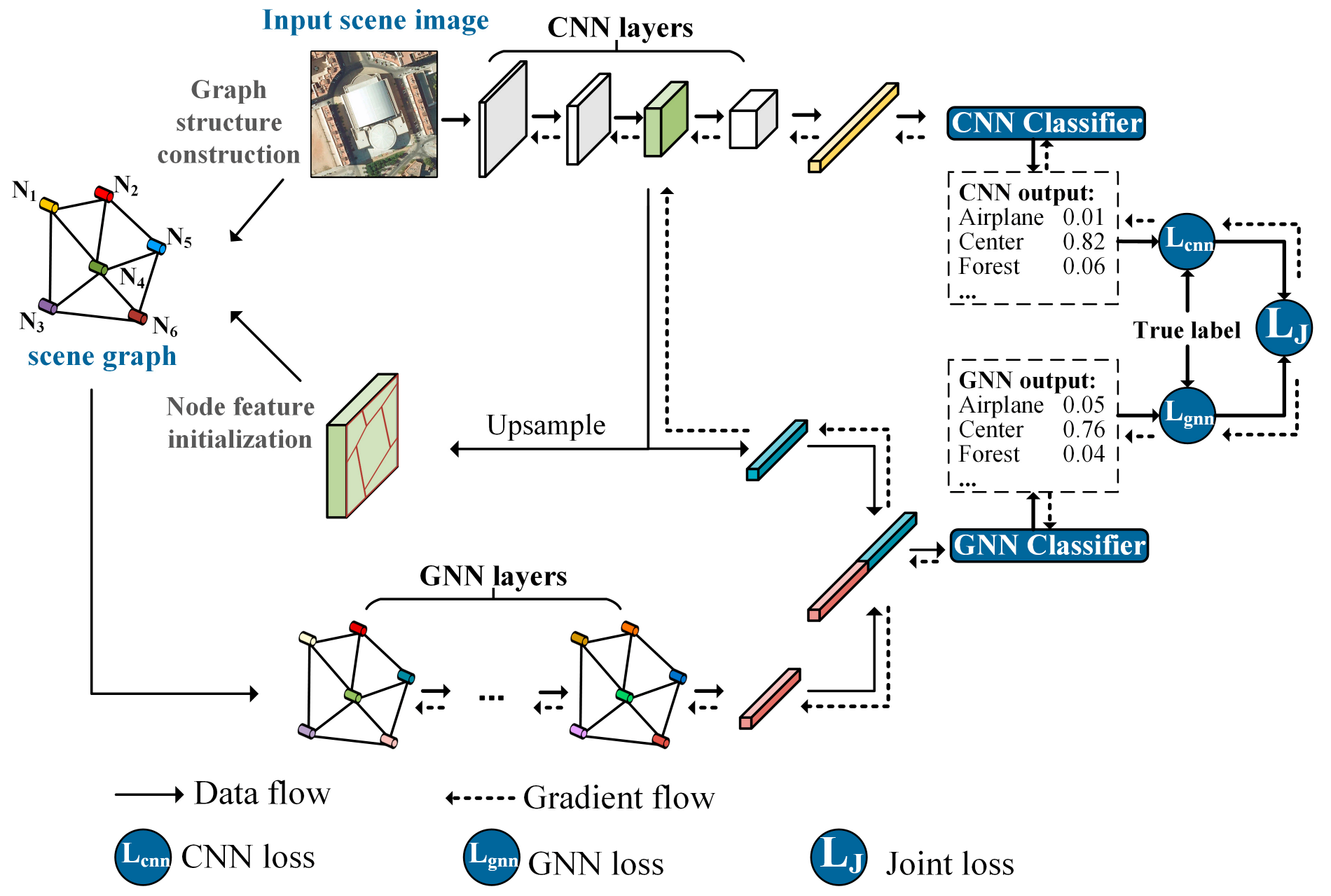
The architecture of our multi-output network (MopNet) combining GNN and CNN for RS scene classification is shown in Figure 2. A graph is created for an RS image through graph structure construction. For the graph, nodes are denoted as corresponding superpixel regions obtained from RS images through image segmentation. The CNN-based branch in MopNet plays the role of a feature extractor for initializing features of graph nodes, and it functions as an encoder of global visual feature representation for RS images. The GNN-based branch in MopNet contributes to aggregating local features into global graph representations by employing the spatial and topological relationships implicit in graph edges. MopNet utilizes two classifiers to output GNN logits and CNN logits. The learnable parameters of the MopNet are optimized by minimizing the joint loss during the training period. In the inference stage, the final prediction of the input scene image is obtained from the GNN-based branch of MopNet. Details of the MopNet are elaborated in the remaining parts of this section.
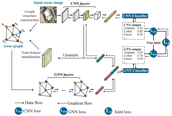
Figure 2.
Architecture of the multi-output network (MopNet) for RS scene classification. In this figure, the category of the chosen example scene is the center.
2.1. Graph Structure Construction
As seen in Figure 3, the graph structure construction procedure abstracts graph-structured information from a regular-shaped image for an RS image. A number of superpixel regions are first obtained from RS images through unsupervised image segmentation. These superpixels are regarded as graph nodes. Graph edges between nodes are created according to the spatial adjacency between corresponding superpixel regions. In this way, each RS image is transformed into a graph.
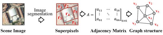
Figure 3.
Illustration of the graph structure construction procedure for an RS image.
Mathematically, the graph of an RS image is symbolized as , where is the set of nodes representing entities, and is the set of edges representing the relationships between entities. A graph can be formed from an adjacency matrix , denoting whether an edge between two corresponding nodes exists or not. For an RS image, the adjacency matrix of a graph is symbolized as , where is the total number of superpixel regions obtained by the unsupervised segmentation method, and is defined as:
where and are two superpixel regions.
2.2. Node Feature Matrix Initialization
After the graph structure has been constructed, the node feature matrix is initialized and used for graph classification. The CNN-based branch of MopNet is used as a feature extractor to yield the feature map to initialize the node features. Typically, the CNN generates multiple feature maps with varying spatial sizes and different numbers of channels. The feature map yields from the intermediate block, such as the block “conv4_x” of ResNet [13], and is selected to initialize the node features. As the spatial size of feature maps decreases, feature maps closer to the output layer contain high-level semantic information but have fewer details, while feature maps closer to the input layer have more detailed features that contain low-level semantic information with some noise [32].
The selected feature map is copied and upsampled to the size of the input RS image. By laying the boundary of superpixel regions over the feature map, each node in the scene graph is assigned the maximum feature value of the corresponding superpixel region. The node feature matrix is symbolized as , where is the th feature value of the th node, and is the length of node features. is calculated as:
where denotes the th superpixel region, i.e., the th node. ( denotes the location of the pixel in , and is the value of the upsampled feature map in the th channel at the location (.
2.3. Encoders and Classifiers in MopNet
MopNet has two encoders, a CNN encoder and a GNN encoder, and their corresponding classifiers. The CNN encoder obtains global visual features for RS images. The GNN encoder obtains global graph representations for scene graphs constructed from RS images.
2.3.1. Global Visual Feature Vector Extraction from the CNN Encoder
For an RS image, two global visual feature vectors are obtained from the CNN encoder using different feature maps of two different blocks. Specifically, feature maps can be obtained via a specified convolutional block of the CNN. Then, global average pooling (GAP) [35] with a fixed output size set at 1 is stacked over these feature maps to calculate global visual feature vectors. The global visual feature vector is symbolized as , where is the number of feature channels of the feature map generated from the th block of the CNN. is calculated as:
where denotes the corresponding spatial range of the th feature map, ( denotes the location of the pixel in , is the total number of pixels in , and is the feature vector with the length of and filtered from the th feature map at the location (.
Two global visual feature vectors obtained from different feature maps of the CNN are separately used in the two classifiers of MopNet. One is generated from the aforementioned intermediate feature map for initializing node features of scene graphs, denoted as in Section 2.3.3, and is later fused with the global graph representation to be fed into a classifier for the GNN output. The other one is generated from the last feature map, denoted as in Section 2.3.3, and is fed into a classifier for the CNN output.
2.3.2. Global Graph Representations from the GNN Encoder
In this paper, two GNN models, the graph convolutional network (GCN) [26] and graph attention network (GAT) [30], are adopted as two different GNN backbones to aggregate local node features of scene graphs generated from RS images. GCN aggregates the node information from neighboring nodes to yield a new feature representation.
Mathematically, is the feature vector of node , where is the number of output channels of the th GNN layer. Thus, the new feature representation of is generated by graph convolution as:
where is the activation function, is the learnable weight matrix, and is the set of neighbors of node . denotes the feature vector of at the th GNN layer. is the product of the square root of node degrees, i.e., .
GAT learns edge weights that reflect to what extent different neighbors contribute to the new representation via a multi-head attention mechanism in an adaptive learning way when aggregating neighboring node features [30]. Correspondingly, in GAT is calculated as follows:
where is the concatenation operation and is the number of attention heads. denotes the normalized weight coefficient between and and is calculated as:
where is the weight coefficient between and its neighbor . is calculated via a fully connected layer as:
where is the fully connected layer with output channels. By integrating Equations (6) and (7), is completely written as:
Global graph pooling is used to generate global graph representations for the scene graph after aggregating node features by graph convolutional layers or graph attention layers. A weight-and-sum pooling layer [36] is used to transform local node features into global graph features for the classification task. The global graph feature vector , where is the number of output channels of the final GNN layer, is calculated as:
where represents a linear transform layer with one output channel and represents the feature vector of output from the final GNN layer.
2.3.3. Multi-Output Logits of MopNet from Classifiers
The MopNet has two classifiers: a classifier with a multilayer perceptron (MLP) for the GNN output and a classifier with a fully connected layer for the CNN output. A concatenation operation is adopted to fuse the global graph feature representation with the global visual feature vector generated from the intermediate feature map. The newly generated feature vector is fed into a two-layer MLP to produce the GNN output. The GNN output is calculated as:
where is the global feature vector generated from the intermediate feature map selected for initializing the node feature matrix.
Additionally, the global feature vector generated from the last feature map of CNN is fed into a fully connected layer to produce the logits as the CNN output , which is calculated as:
where is the number of scene classes and denotes a fully connected layer with output channels.
2.4. Loss Function of MopNet
The MopNet is trained with the joint loss . is calculated by integrating the GNN loss and the CNN loss with a balance parameter as:
where denotes model parameters, including GNN parameters , CNN parameters , and parameters of classifiers . and are separately calculated via a cross-entropy function. In this paper, label smoothing [37] is further adopted to reduce overfitting effects and improve prediction accuracy. The joint loss is rewritten as:
where denotes the smoothed label, calculated from one-hot label according to [37]. and are separately calculated as:
where denotes the number of scene classes and represents the weights and bias of the last layer.
In our MopNet, learnable parameters of the GNN and the CNN are simultaneously optimized by backward propagation during the training process of the model. The training process of MopNet is depicted in Algorithm 1. The adjacent matrix and the superpixel regions are obtained during graph structure construction, which is performed before the training process of the MopNet.
| Algorithm 1. Training process of MopNet. |
| Input: RS images I, adjacent matrix A, segmented superpixel regions R and true labels y in training set. Output: GNN parameters , CNN parameters and parameters of classifiers . Learning MopNet:
|
3. Experiments and Results
The results of our experiments are presented and analyzed in this section. A description of the datasets used in this paper can be found in Section 3.1. The experimental settings are then described in Section 3.2. In Section 3.3, the experimental results on two public datasets are provided and compared with the results of the state-of-the-art methods.
3.1. Experimental Data Sets
Two RS image scene classification benchmark datasets were employed to test the effectiveness of the MopNet. The characteristics of the two used datasets are listed in Table 1.

Table 1.
Characteristics of the two RS image scene classification datasets used in this study.
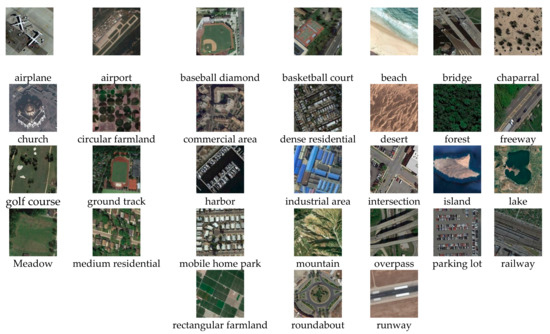
Figure 4.
Example images of the OPTIMAL-31 dataset.
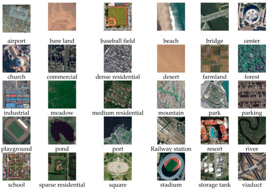
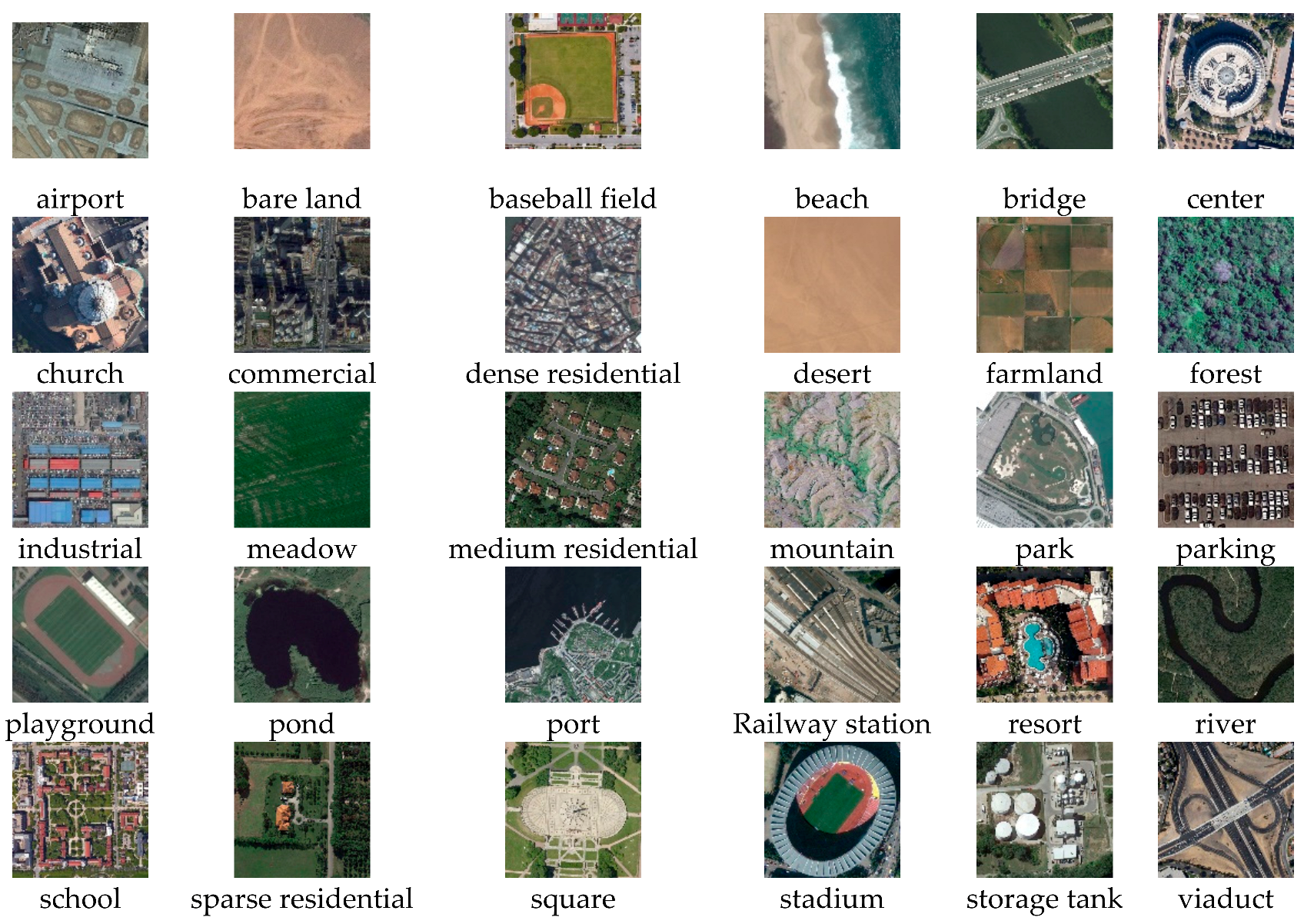
Figure 5.
Example images of the AID dataset.
3.2. Experimental Settings
For MopNet, GAT and GCN were separately used as the GNN backbone, while ResNet50 was used as the CNN backbone. The MopNet without the CNN prediction, identified as SopNet, was also compared with the MopNet. Specifically, the following four experiments were conducted in our study: MopNet-GAT-ResNet50, MopNet-GCN-ResNet50, SopNet-GAT-ResNet50, and SopNet-GCN-ResNet50.
Some parameters in our method were set as follows. Felzenszwalb’s algorithm [40] was applied to generate superpixel regions from RS images in the graph structure construction, with the segmentation scale set as 50 and 300 for the OPTIMAL-31 and AID datasets, respectively. The GCN encoder used had two graph convolutional layers, while the GAT encoder used had two graph attention convolutional layers with eight attention heads. In these two GNN encoders, the hidden dimension and output dimension were both 512. The feature map from block “conv4_x” of ResNet50 was chosen for initializing node feature matrixes for scene graphs. All the experiments were trained for 100 epochs. Adam was used as the optimizer, and the learning rate was 1e-3. The mini-batch sizes were 16 and 8 for the OPTIMAL-31 and AID datasets, respectively.
Our model was implemented using PyTorch and the Deep Graph Library (DGL) [41]. All experiments were conducted on a personal computer equipped with an Intel core i9-10900K CPU and NVIDIA GeForce RTX 3090 GPU with 24 GB of memory.
3.3. Scene Classification Results
3.3.1. Results under Different Balance Parameters
To determine how the balance parameter of the joint loss affects the classification results, different values were set in MopNet-GAT-ResNet50 on the OPTIMAL-31 dataset. Table 2 shows the results when increased from 0.1 to 0.9. In general, as increased, the accuracy first fluctuated and then decreased. The highest overall accuracy (OA) of 96.06% was obtained when was 0.7. This indicates that both GNN-based and CNN-based branches contributed to improving the scene classification performance of MopNet but did not contribute equally. The GNN-based or CNN-based branch should not be given a fully dominant weight. In the following experiments, was set as 0.7.
Table 2.
Overall accuracy on the OPTIMAL-31 dataset with different balance parameters of the joint loss by MopNet-GAT-ResNet50.
3.3.2. Results of MopNet on the OPTIMAL-31 Dataset
Quantitative results are presented for the OPTIMAL-31 dataset in Table 3. OA values of 96.06% and 95.34% were achieved by MopNet-GAT-ResNet50 and MopNet-GCN-ResNet50, outperforming the fine-tuned ResNet50 with increases of 5.60% and 4.88%, respectively. Generally, MopNet-GAT-ResNet50 had a higher OA and lower standard deviations than MopNet-GCN-ResNet50, indicating better performance and the robustness of using GAT as the GNN backbone on the OPTIMAL-31 dataset. Nevertheless, both MopNet-GAT-ResNet50 and MopNet-GCN-ResNet50 achieved better results than most of the compared methods in Table 3. Notably, our MopNet-GAT-ResNet50 obtained a higher accuracy than the method in [42] using the vision transformer, which has achieved remarkable performances on classification tasks in recent years.
Table 3.
Comparison of OAs (%) on the OPTIMAL-31 dataset.
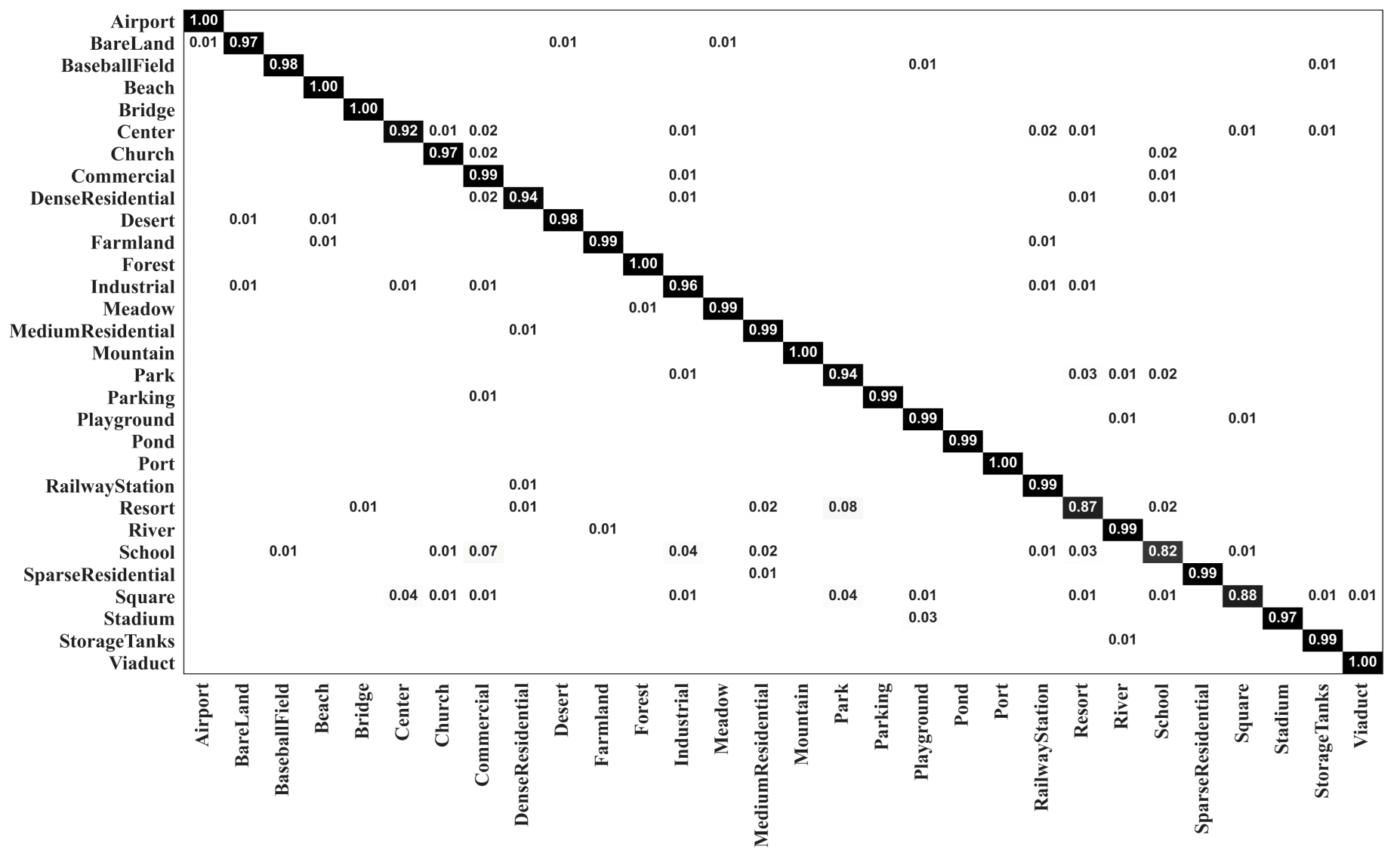
The confusion matrix generated by MopNet-GAT-ResNet50 on the OPTIMAL-31 dataset is presented in Figure 6. It can be seen that 28 out of 31 categories had scores higher than 90%, with 21 categories having scores of 100%. MopNet-GAT-ResNet50 had a better ability to discriminate the classes that are easily misclassified by other methods, such as DM-GAF [23]. The commercial area, dense residential area, and industrial area were classified by our model with accuracies of 92%, 83%, and 100%, respectively, while these three classes only obtained accuracies of 83%, 67%, and 83%, respectively, by DM-GAF [23].
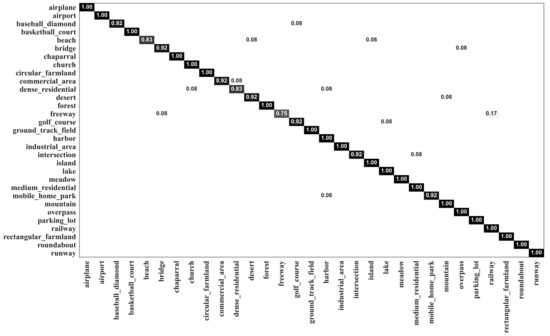
Figure 6.
Confusion matrix of MopNet-GAT-ResNet50 on the OPTIMAL-31 dataset.
3.3.3. Results of MopNet on the AID Dataset
A comparison of the results on the AID dataset is presented in Table 4. Our MopNet had a comparable or even better performance on the AID dataset than the methods presented in Table 4. On the AID dataset, MopNet-GCN-ResNet50 achieved a higher OA than MopNet-GAT-ResNet50 under training ratios of 20% and 50%, with OA values of 95.53% and 97.11%, respectively. Our MopNet obtained much better results than DM-GAF on the AID dataset, although our MopNet had a slightly lower OA than DM-GAF on the OPTIMAL dataset. In addition, our MopNet obtained greater improvements under a training ratio of 20% than under a training ratio of 50% compared with methods such as SFCNN [47], DCNN [10], and the method combining CNN with GCN [32]. This phenomenon indicates that our MopNet is robust for scene classification, especially when the training set is small.
Table 4.
Comparison of OAs (%) of different methods on the AID dataset.
Figure 7 and Figure 8 show the confusion matrixes generated by our MopNet-GCN-ResNet50 on the AID dataset under training ratios of 20% and 50%, respectively. The number of categories with classification accuracies higher than 95% was 22 and 24 under the training ratios of 20% and 50%, respectively. The most obvious misclassification occurred between the categories of resort and park, and between the categories of school and commercial area. Taking the results under the training ratio of 20% as an example, 4% of the images from the resort were misclassified as parks, and 3% of the images from the school were misclassified as commercial. Similar confusion also occurred for IDCCP [46] and the method combining GCN with CNN [32]. Nevertheless, our MopNet performed better in classifying these confusable categories than these two methods. Specifically, for IDCCP [46], 16% of images from the resort were classified as parks, and 6% of images from the school were classified as commercial. For the method combining a GCN with a CNN [32], 6% of the images from the resort were classified as parks, and 3% of the images from the school were classified as commercial.
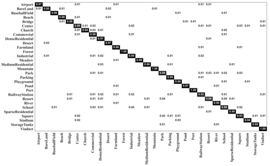
Figure 7.
Confusion matrix of MopNet-GCN-ResNet50 on the AID dataset under a training ratio of 20%.

Figure 8.
Confusion matrix of MopNet-GCN-ResNet50 on the AID dataset under a training ratio of 50%.
3.3.4. Comparison Results of MopNet and SopNet
As seen from the experimental results, our MopNet obtained higher OAs with lower standard deviations than the corresponding SopNet. Specifically, as shown in Table 3, on the OPTIMAL-31 dataset, our MopNet with GCN and GAT as the GNN backbones obtained 1.97% and 2.69% improvements in OA compared to SopNet, respectively. According to Table 4, on the AID dataset, MopNet with GCN obtained 6.55% and 3.55% improvements in OA under the 20% and 50% training ratios compared to SopNet, respectively, while MopNet with GAT obtained 3.9% and 1.59% improvements. Moreover, MopNet obtained lower standard deviations of OAs than the corresponding SopNet.
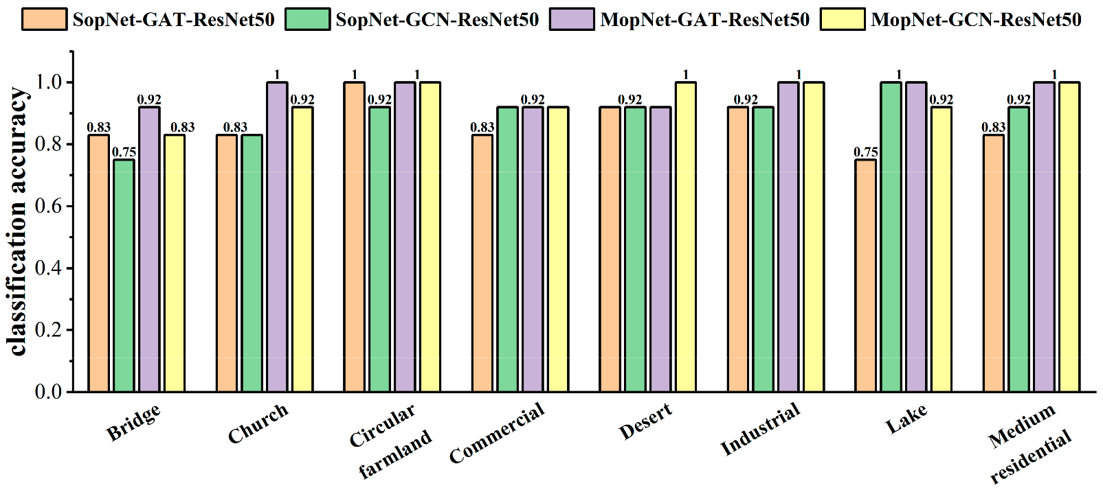
The classification accuracies obtained by MopNet and SopNet for some typical categories are presented in Figure 9, Figure 10 and Figure 11. Some categories with complex spatial and topological relations among ground objects in the scene images were selected for comparison, such as church, commercial area, industrial area, center, school, square, and residential area. Some categories with no salient spatial topological dependences contained in the scene images, such as desert, lake, and bare land, were also selected for comparison. As seen in Figure 9, Figure 10 and Figure 11, MopNet usually obtained higher classification accuracies than the corresponding SopNet for these categories on the two datasets.
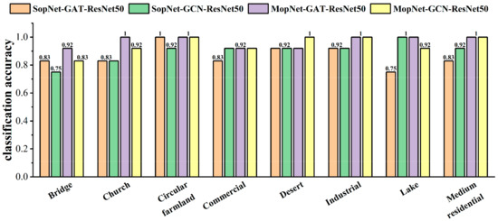
Figure 9.
Classification accuracies calculated by MopNet and SopNet on some typical classes of the OPTIMAL-31 dataset.
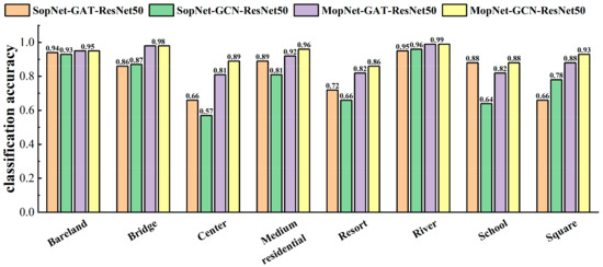
Figure 10.
Classification accuracies calculated by MopNet and SopNet on some typical classes of the AID dataset under the training ratio of 20%.
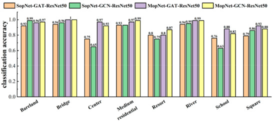
Figure 11.
Classification accuracies calculated by MopNet and SopNet on some typical classes of the AID dataset under the training ratio of 50%.
4. Discussion
4.1. Effectiveness of MopNet for Various Categories
The proposed MopNet had universally promising performance for various categories of RS scenes. As seen in Figure 6, Figure 7 and Figure 8, our MopNet had a robust capability in classifying various categories of scenes, although different categories of scenes usually have various geographical entities and spatial distributions among these entities. The number of graph nodes generated from an RS image is related to the number of geographical entities in these images. The average and the variance of graph node counts of various categories are presented in Table 5 and Table 6. Complex RS scenes, such as dense residential scenes, usually had more graph nodes, while simple RS scenes, such as meadow scenes, usually had fewer graph nodes. For a specified category, the spatial and topological relationships imbedded in images of the category were imbedded in graph edges between corresponding nodes and were employed through the message propagation mechanism of MopNet. In this way, the MopNet was effective at scene classification for various categories.
Table 5.
Node counts of each category in the OPTIMAL-31 dataset.
Table 6.
Node counts of each category in the AID dataset.
As seen in Table 5, for the OPTIMAL-31 dataset, the categories of commercial, dense residential, industrial, and medium residential had a larger number of graph nodes. It was difficult for RS scene classification methods to distinguish these categories. Our MopNet obtained accuracies of 92%, 83%, 100%, and 100% for these categories, respectively, which are comparable to or higher than existing methods, such as DM-GAF [23]. In contrast, the category of island generated fewer graph nodes and was relatively easy to classify. For the island, our MopNet obtained a classification accuracy of 100%, while DM-GAF [23] obtained an accuracy of 83%.
As seen in Table 6, for the AID dataset, the commercial, dense residential, and industrial categories had abundant details in the scene images and thus had a large number of graph nodes. For these categories, our MopNet obtained accuracies of 98%, 97%, and 95%, respectively, under the training ratio of 20%, while the results generated by the method combining GCN with CNN [32] were 95%, 91%, and 94%, respectively. In contrast, categories such as desert and meadow had poor textures and thus had the fewest graph nodes. Our MopNet obtained accuracies of 97% and 99% separately for these two categories, while the method in [32] obtained accuracies of 92% and 98%, respectively.
4.2. Contribution of the GNN and CNN in MopNet to Scene Classification
Both the GNN-based and CNN-based branches of MopNet contribute to RS image scene classification but do not contribute equally. The contributions of the GNN and CNN are described as follows:
- (1)
- The GNN-based branch employs spatial and topological relationships imbedded in RS images, leading to an improved classification accuracy of MopNet. The GNN compensates for the shortcoming of the CNN by representing features in non-Euclidean space. Given that the balance parameter λ was suggested to be set as 0.7 by the comparison experiments, the GNN plays an important role in minimizing the joint loss of the MopNet. Moreover, the contribution of the GNN to MopNet can also be drawn from the comparison between our MopNet and GLDBS [34]. GLDBS [34] used two CNNs as the backbones of two branches, unlike our MopNet, which has a GNN branch beside a CNN branch. It is difficult for models such as GLDBS to effectively learn the spatial and topological information. The experimental results show that our MopNet obtained higher overall accuracies than GLDBS on the AID dataset.
- (2)
- The CNN-based branch helps to improve the performance and stability of MopNet. As shown in Table 3 and Table 4, MopNet obtained higher overall accuracies (OAs) and lower standard deviations of OAs in comparison to the corresponding SopNet, which did not involve the CNN prediction in the optimized objective of the model. As shown in Figure 9, Figure 10 and Figure 11, MopNet achieved obvious accuracy improvements in comparison to the corresponding SopNet for various categories, such as commercial and industrial in the OPTIMAL-31 dataset and center, resort, school, and square in the AID dataset. SopNet suffers from the effect of uncertainties caused by image segmentation and graph structure construction for images of these categories. For MopNet, the CNN-based branch helps to reduce the effect and thus improve the stability.
4.3. Differences between MopNets and Existing Methods Combining CNN and GNN
The proposed MopNet differs from the existing methods that also combine CNN and GNN [24,32] in terms of the training strategy and the prediction output.
- (1)
- Training strategy: A training strategy of jointly learning CNN and GNN was adopted in MopNet. The parameters of the CNN and GNN in MopNet are updated simultaneously with the guidance of a joint loss via the backpropagation mechanism. In contrast, the method in [24] adopts the step-by-step training strategy, training the CNN and the GNN separately. The parameters of the CNN and GNN in [24] were not simultaneously optimized as in our MopNet. The classification performance of the GNN in [24] may suffer from the effect of the representation ability of the CNN.
- (2)
- Prediction output: The experimental results indicate that the MopNet obtained higher classification accuracies with more robustness than the corresponding SopNet that did not involve the CNN output in the optimized objective. Moreover, our MopNet regarded both outputs of the GNN and CNN as the optimized objective, unlike the method in [32] using the GNN prediction alone. Our MopNet obtained better classification results than the method in [32]. In the future, MopNet will be investigated with more CNN backbones and various GNN backbones.
5. Conclusions
In this paper, a new multi-output network (MopNet) combining GNN and CNN is proposed for achieving high-accuracy RS image scene classification. The parameters of the CNN and GNN in MopNet are updated simultaneously with the guidance of a joint loss via the backpropagation mechanism. Experimental results on the OPTIMAL-31 and AID datasets show that the proposed MopNet combining GAT/GCN and ResNet50 has promising overall accuracies, outperforming the state-of-the-art methods. The proposed MopNet is able to achieve higher overall accuracies with lower variances than the corresponding single-output network (SopNet). The CNN-based branch of MopNet reduces the effect of uncertainties caused by image segmentation and graph structure construction for RS images, and thus helps to improve the performance and stability of MopNet. On the other hand, the GNN-based branch employs spatial and topological relationships imbedded in graph edges among geographical objects in RS images and helps to improve the classification accuracy of MopNet. Spatial and topological relationships imbedded in RS images are helpful for improving the performance of scene classification.
Author Contributions
Conceptualization, F.P.; methodology, F.P. and W.L.; software, W.L.; validation, K.Q., X.Z. and Q.Z.; formal analysis, F.P. and W.L.; investigation, F.P. and K.Q.; resources, F.P. and X.Z.; data curation, Q.Z.; writing—original draft preparation, F.P. and W.L.; writing—review and editing, F.P. and W.T.; visualization, W.L.; supervision, F.P.; project administration, F.P.; funding acquisition, F.P. All authors have read and agreed to the published version of the manuscript.
Funding
This work was supported by the National Natural Science Foundation of China under Grants 42071389, 41701511, and 41801323 and the Fundamental Research Funds for the Central Universities under Grant CCNU20TS033.
Institutional Review Board Statement
Not applicable.
Informed Consent Statement
Not applicable.
Data Availability Statement
The OPTIMAL-31 dataset was acquired at the website http://crabwq.github.io (accessed on 8 February 2022). The Aerial Image Dataset (AID) dataset was acquired at the website https://captain-whu.github.io/AID (accessed on 8 February 2022).
Conflicts of Interest
The authors declare no conflict of interest.
References
- Cheng, G.; Xie, X.; Han, J.; Xia, G.S. Remote sensing image scene classification meets deep learning: Challenges, methods, benchmarks, and opportunities. IEEE J. Sel. Top. Appl. Earth Obs. Remote Sens. 2020, 13, 3735–3756. [Google Scholar] [CrossRef]
- Egenhofer, M.J.; Franzosa, R.D. Point-set topological spatial relations. Int. J. Geogr. Inf. Syst. 1991, 5, 161–174. [Google Scholar] [CrossRef] [Green Version]
- Zhu, Q.; Zhong, Y.; Zhao, B.; Xia, G.; Zhang, L. Bag-of-Visual-Words Scene Classifier with Local and Global Features for High Spatial Resolution Remote Sensing Imagery. IEEE Geosci. Remote Sens. Lett. 2016, 13, 747–751. [Google Scholar] [CrossRef]
- Zhao, L.J.; Tang, P.; Huo, L.Z. Land-use scene classification using a concentric circle-structured multiscale bag-of-visual-words model. IEEE J. Sel. Top. Appl. Earth Obs. Remote Sens. 2014, 7, 4620–4631. [Google Scholar] [CrossRef]
- Dong, R.; Xu, D.; Jiao, L.; Zhao, J.; An, J. A Fast Deep Perception Network for Remote Sensing Scene Classification. Remote Sens. 2020, 12, 729. [Google Scholar] [CrossRef] [Green Version]
- Chen, J.; Wang, C.; Ma, Z.; Chen, J.; He, D.; Ackland, S. Remote Sensing Scene Classification Based on Convolutional Neural Networks Pre-Trained Using Attention-Guided Sparse Filters. Remote Sens. 2018, 10, 290. [Google Scholar] [CrossRef] [Green Version]
- Hu, F.; Xia, G.-S.; Hu, J.; Zhang, L. Transferring Deep Convolutional Neural Networks for the Scene Classification of High-Resolution Remote Sensing Imagery. Remote Sens. 2015, 7, 14680–14707. [Google Scholar] [CrossRef] [Green Version]
- Gu, Y.; Wang, Y.; Li, Y. A Survey on Deep Learning-Driven Remote Sensing Image Scene Understanding: Scene Classification, Scene Retrieval and Scene-Guided Object Detection. Appl. Sci. 2019, 9, 2110. [Google Scholar] [CrossRef] [Green Version]
- Pires de Lima, R.; Marfurt, K. Convolutional Neural Network for Remote-Sensing Scene Classification: Transfer Learning Analysis. Remote Sens. 2020, 12, 86. [Google Scholar] [CrossRef] [Green Version]
- Cheng, G.; Yang, C.; Yao, X.; Guo, L.; Han, J. When Deep Learning Meets Metric Learning: Remote Sensing Image Scene Classification via Learning Discriminative CNNs. IEEE Trans. Geosci. Remote Sens. 2018, 56, 2811–2821. [Google Scholar] [CrossRef]
- Akodad, S.; Bombrun, L.; Xia, J.; Berthoumieu, Y.; Germain, C. Ensemble Learning Approaches Based on Covariance Pooling of CNN Features for High Resolution Remote Sensing Scene Classification. Remote Sens. 2020, 12, 3292. [Google Scholar] [CrossRef]
- Simonyan, K.; Zisserman, A. Very deep convolutional networks for large-scale image recognition. arXiv 2014, arXiv:1409.1556. [Google Scholar]
- He, K.; Zhang, X.; Ren, S.; Sun, J. Deep residual learning for image recognition. In Proceedings of the 2016 IEEE Conference on Computer Vision and Pattern Recognition (CVPR), Las Vegas, NV, USA, 27–30 June 2016. [Google Scholar] [CrossRef] [Green Version]
- Huang, G.; Liu, Z.; Van Der Maaten, L.; Kilian, Q.W. Densely connected convolutional networks. In Proceedings of the 2017 IEEE Conference on Computer Vision and Pattern Recognition (CVPR), Honolulu, HI, USA, 21–26 July 2017. [Google Scholar] [CrossRef] [Green Version]
- Krizhevsky, A.; Sutskever, I.; Hinton, G.E. Imagenet classification with deep convolutional neural networks. Adv. Neural Inf. Process. Syst. 2012, 25, 1097–1105. [Google Scholar] [CrossRef]
- Zhao, X.; Zhang, J.; Tian, J.; Zhuo, L.; Zhang, J. Residual Dense Network Based on Channel-Spatial Attention for the Scene Classification of a High-Resolution Remote Sensing Image. Remote Sens. 2020, 12, 1887. [Google Scholar] [CrossRef]
- Zhang, W.; Tang, P.; Zhao, L. Remote Sensing Image Scene Classification Using CNN-CapsNet. Remote Sens. 2019, 11, 494. [Google Scholar] [CrossRef] [Green Version]
- Li, J.; Lin, D.; Wang, Y.; Xu, G.; Zhang, Y.; Ding, C.; Zhou, Y. Deep Discriminative Representation Learning with Attention Map for Scene Classification. Remote Sens. 2020, 12, 1366. [Google Scholar] [CrossRef]
- Shi, C.; Zhao, X.; Wang, L. A Multi-Branch Feature Fusion Strategy Based on an Attention Mechanism for Remote Sensing Image Scene Classification. Remote Sens. 2021, 13, 1950. [Google Scholar] [CrossRef]
- Li, M.; Lei, L.; Tang, Y.; Sun, Y.; Kuang, G. An Attention-Guided Multilayer Feature Aggregation Network for Remote Sensing Image Scene Classification. Remote Sens. 2021, 13, 3113. [Google Scholar] [CrossRef]
- Li, Q.; Yan, D.; Wu, W. Remote Sensing Image Scene Classification Based on Global Self-Attention Module. Remote Sens. 2021, 13, 4542. [Google Scholar] [CrossRef]
- Xu, C.; Zhu, G.; Shu, J. A Lightweight and Robust Lie Group-Convolutional Neural Networks Joint Representation for Remote Sensing Scene Classification. IEEE Trans. Geosci. Remote Sens. 2022, 60, 1–15. [Google Scholar] [CrossRef]
- Shen, J.; Zhang, T.; Wang, Y.; Wang, R.; Wang, Q.; Qi, M. A Dual-Model Architecture with Grouping-Attention-Fusion for Remote Sensing Scene Classification. Remote Sens. 2021, 13, 433. [Google Scholar] [CrossRef]
- Li, Y.; Chen, R.; Zhang, Y.; Zhang, M.; Chen, L. Multi-Label Remote Sensing Image Scene Classification by Combining a Convolutional Neural Network and a Graph Neural Network. Remote Sens. 2020, 12, 4003. [Google Scholar] [CrossRef]
- Manzo, M.; Rozza, A. DOPSIE: Deep-Order Proximity and Structural Information Embedding. Mach. Learn. Knowl. Extr. 2019, 1, 684–697. [Google Scholar] [CrossRef] [Green Version]
- Wu, Z.; Pan, S.; Chen, F.; Long, G.; Zhang, C.; Yu, P.S. A comprehensive survey on graph neural networks. IEEE Trans. Neural Netw. Learn. Syst. 2020, 32, 4–24. [Google Scholar] [CrossRef] [Green Version]
- Gao, Y.; Shi, J.; Li, J.; Wang, R. Remote sensing scene classification based on high-order graph convolutional network. Eur. J. Remote Sens. 2021, 54 (Suppl. S1), 141–155. [Google Scholar] [CrossRef]
- Ouyang, S.; Li, Y. Combining Deep Semantic Segmentation Network and Graph Convolutional Neural Network for Semantic Segmentation of Remote Sensing Imagery. Remote Sens. 2021, 13, 119. [Google Scholar] [CrossRef]
- Liu, H.; Xu, D.; Zhu, T.; Shang, F.; Liu, Y.; Lu, J.; Yang, R. Graph Convolutional Networks by Architecture Search for PolSAR Image Classification. Remote Sens. 2021, 13, 1404. [Google Scholar] [CrossRef]
- Veličković, P.; Cucurull, G.; Casanova, A.; Romero, A.; Liò, P.; Bengio, Y. Graph attention networks. arXiv 2017, arXiv:1710.10903. [Google Scholar]
- Yang, P.; Tong, L.; Qian, B.; Gao, Z.; Yu, J.; Xiao, C. Hyperspectral Image Classification with Spectral and Spatial Graph Using Inductive Representation Learning Network. IEEE J. Sel. Top. Appl. Earth Obs. Remote Sens. 2021, 14, 791–800. [Google Scholar] [CrossRef]
- Liang, J.; Deng, Y.; Zeng, D. A Deep Neural Network Combined CNN and GCN for Remote Sensing Scene Classification. IEEE J. Sel. Top. Appl. Earth Obs. Remote Sens. 2020, 13, 4325–4338. [Google Scholar] [CrossRef]
- Ren, X.; Malik, J. Learning a classification model for segmentation, Computer Vision. In Proceedings of the Ninth IEEE International Conference on Computer Vision, Nice, France, 13–16 October 2003. [Google Scholar]
- Xu, K.; Huang, H.; Deng, P. Remote Sensing Image Scene Classification Based on Global-Local Dual-Branch Structure Model. IEEE Geosci. Remote Sens. Lett. 2021, 19, 1–5. [Google Scholar] [CrossRef]
- Lin, M.; Chen, Q.; Yan, S. Network in network. arXiv 2013, arXiv:1312.4400. [Google Scholar]
- Kipf, T.N.; Welling, M. Semi-supervised classification with graph convolutional networks. arXiv 2016, arXiv:1609.02907. [Google Scholar]
- Müller, R.; Kornblith, S.; Hinton, G. When does label smoothing help? arXiv 2019, arXiv:1906.02629. [Google Scholar]
- Wang, Q.; Liu, S.; Chanussot, J.; Li, X. Scene Classification with Recurrent Attention of VHR Remote Sensing Images. IEEE Trans. Geosci. Remote Sens. 2018, 57, 1155–1167. [Google Scholar] [CrossRef]
- Xia, G.S.; Hu, J.; Hu, F.; Shi, B.; Bai, X.; Zhong, Y.; Zhang, L.; Lu, X. AID: A benchmark data set for performance evaluation of aerial scene classification. IEEE Trans. Geosci. Remote Sens. 2017, 55, 3965–3981. [Google Scholar] [CrossRef] [Green Version]
- Felzenszwalb, P.F.; Huttenlocher, D.P. Efficient Graph-Based Image Segmentation. Int. J. Comput. Vis. 2004, 59, 167–181. [Google Scholar] [CrossRef]
- Wang, M.; Zheng, D.; Ye, Z.; Gan, Q.; Li, M.; Song, X.; Zhou, J.; Ma, C.; Yu, L.; Gai, Y.; et al. Deep graph library: A graph-centric, highly-performant package for graph neural networks. arXiv 2019, arXiv:1909.01315. [Google Scholar]
- Bazi, Y.; Bashmal, L.; Rahhal, M.M.A.; Dayil, R.A.; Ajlan, N.A. Vision Transformers for Remote Sensing Image Classification. Remote Sens. 2021, 13, 516. [Google Scholar] [CrossRef]
- Lv, Y.; Zhang, X.; Xiong, W.; Cui, Y.; Cai, M. An End-to-End Local-Global-Fusion Feature Extraction Network for Remote Sensing Image Scene Classification. Remote Sens. 2019, 11, 3006. [Google Scholar] [CrossRef] [Green Version]
- Liu, N.; Celik, T.; Li, H.C. MSNet: A Multiple Supervision Network for Remote Sensing Scene Classification. IEEE Geosci. Remote Sens. Lett. 2020, 19, 1–5. [Google Scholar] [CrossRef]
- Bazi, Y.; Al Rahhal, M.M.; Alhichri, H.; Alajlan, N. Simple Yet Effective Fine-Tuning of Deep CNNs Using an Auxiliary Classification Loss for Remote Sensing Scene Classification. Remote Sens. 2019, 11, 2908. [Google Scholar] [CrossRef] [Green Version]
- Wang, S.; Ren, Y.; Parr, G.; Guan, Y.; Shao, L. Invariant Deep Compressible Covariance Pooling for Aerial Scene Categorization. IEEE Trans. Geosci. Remote Sens. 2021, 59, 6549–6561. [Google Scholar] [CrossRef]
- Xie, J.; He, N.; Fang, L.; Plaza, A. Scale-Free Convolutional Neural Network for Remote Sensing Scene Classification. IEEE Trans. Geosci. Remote Sens. 2019, 57, 6916–6928. [Google Scholar] [CrossRef]
- Tang, X.; Ma, Q.; Zhang, X.; Liu, F.; Ma, J.; Jiao, L. Attention consistent network for remote sensing scene classification. IEEE J. Sel. Top. Appl. Earth Obs. Remote Sens. 2021, 14, 2030–2045. [Google Scholar] [CrossRef]


Publisher’s Note: MDPI stays neutral with regard to jurisdictional claims in published maps and institutional affiliations. |
© 2022 by the authors. Licensee MDPI, Basel, Switzerland. This article is an open access article distributed under the terms and conditions of the Creative Commons Attribution (CC BY) license (https://creativecommons.org/licenses/by/4.0/).