
Combination of Models to Generate the First PAR Maps for Spain

 ,
,  , , and
Abstract
1. Introduction
2. Materials and Methods
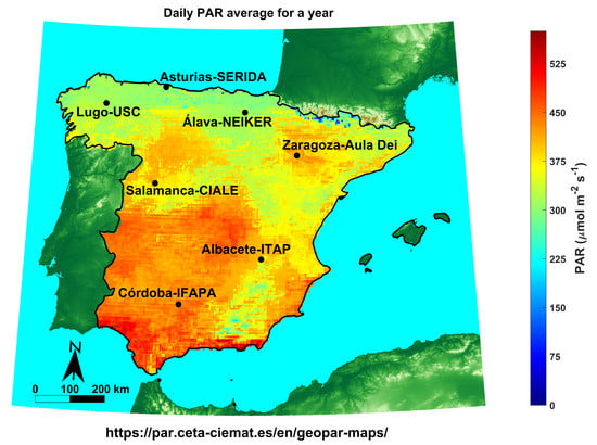
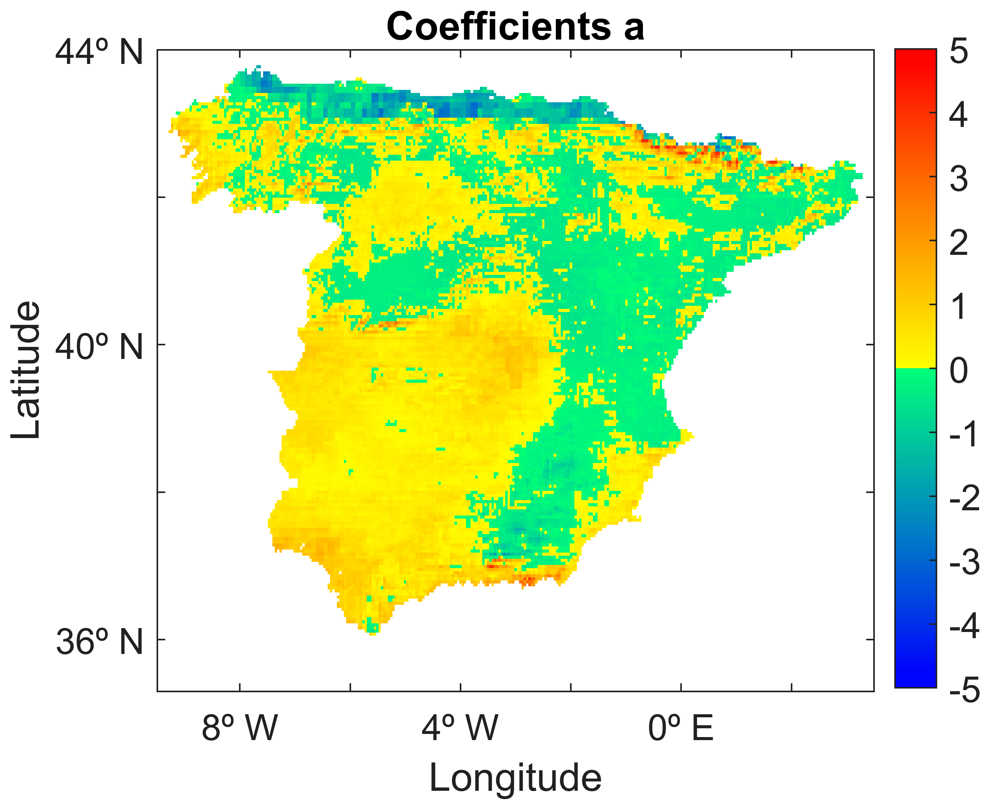
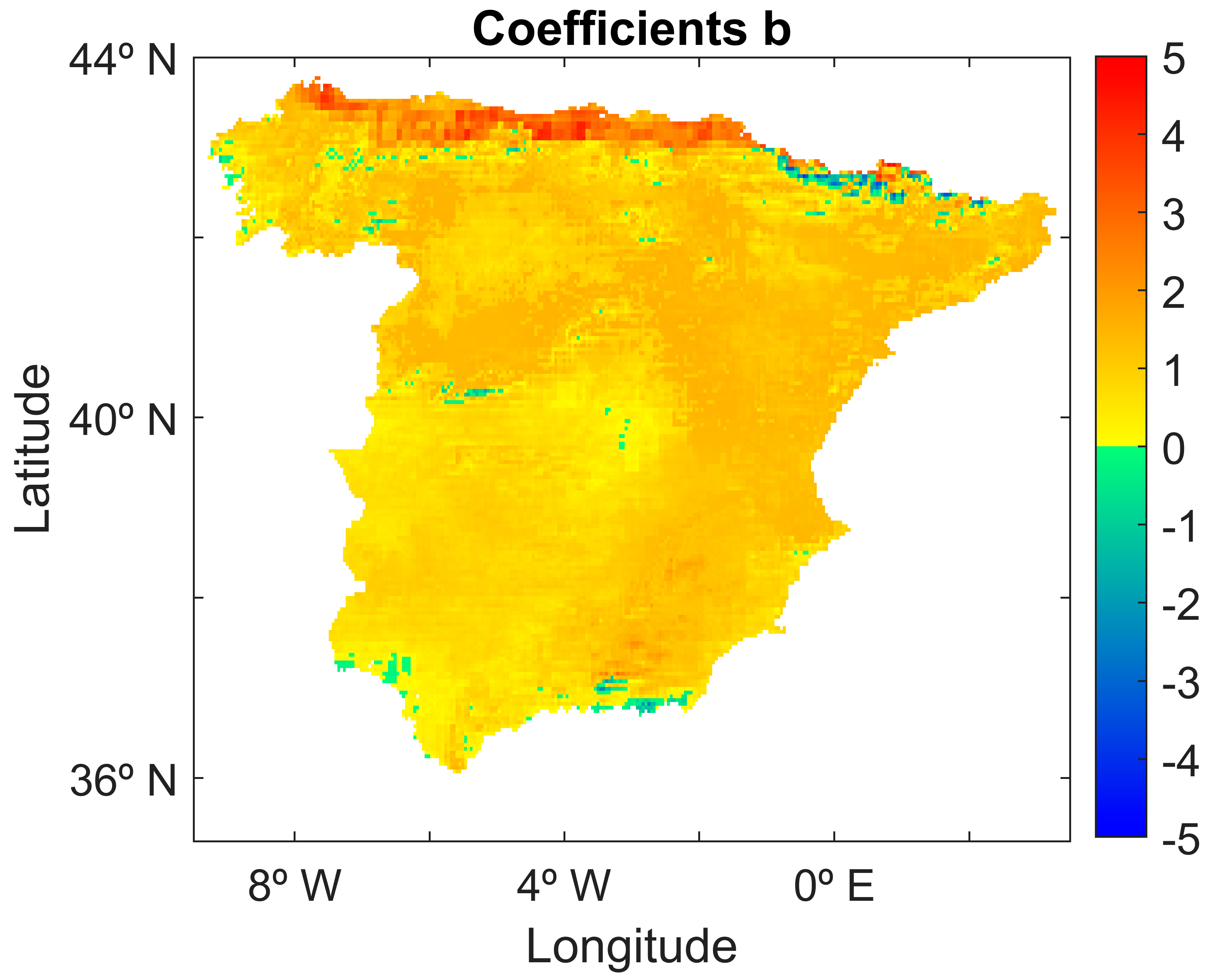
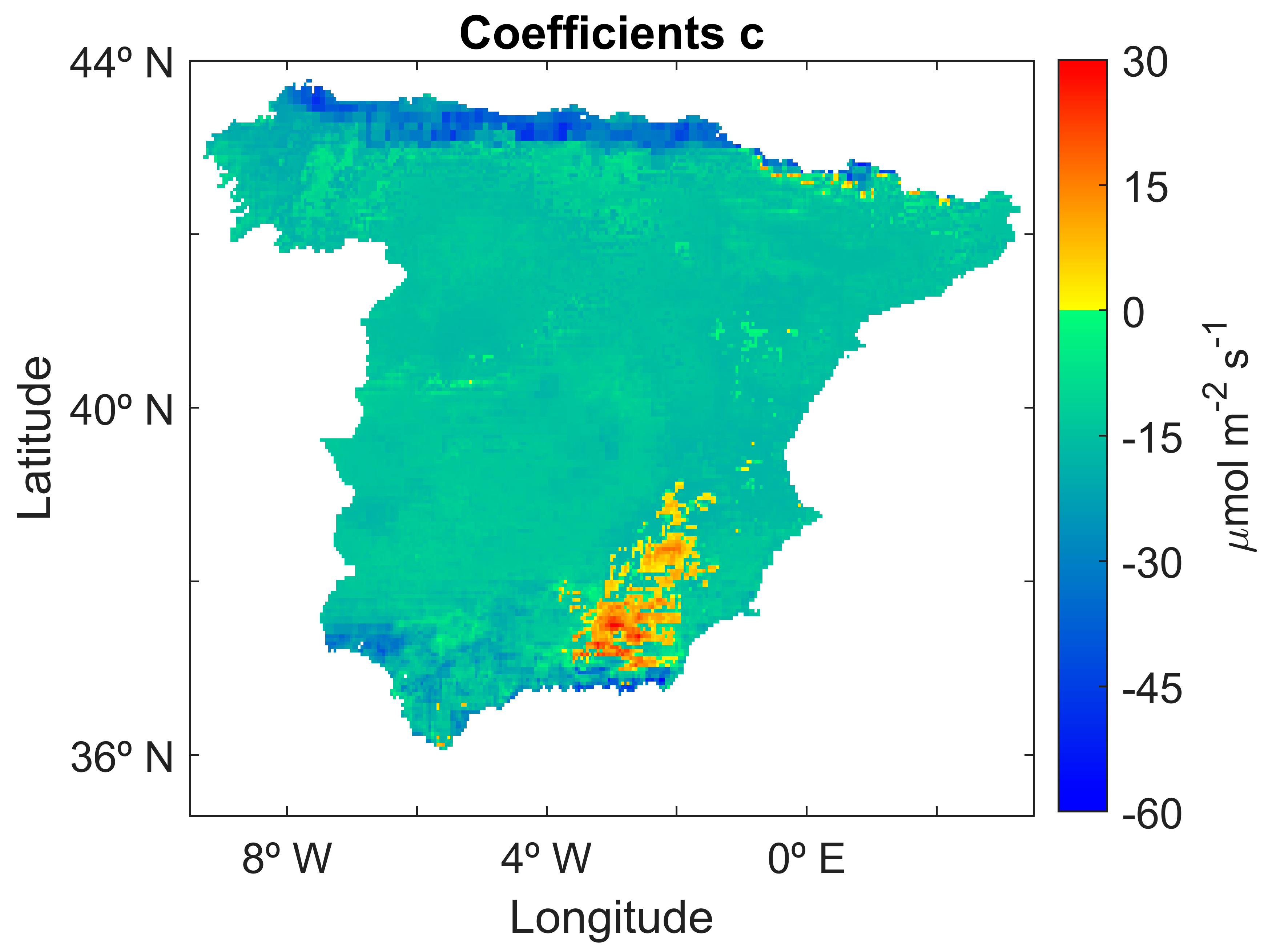
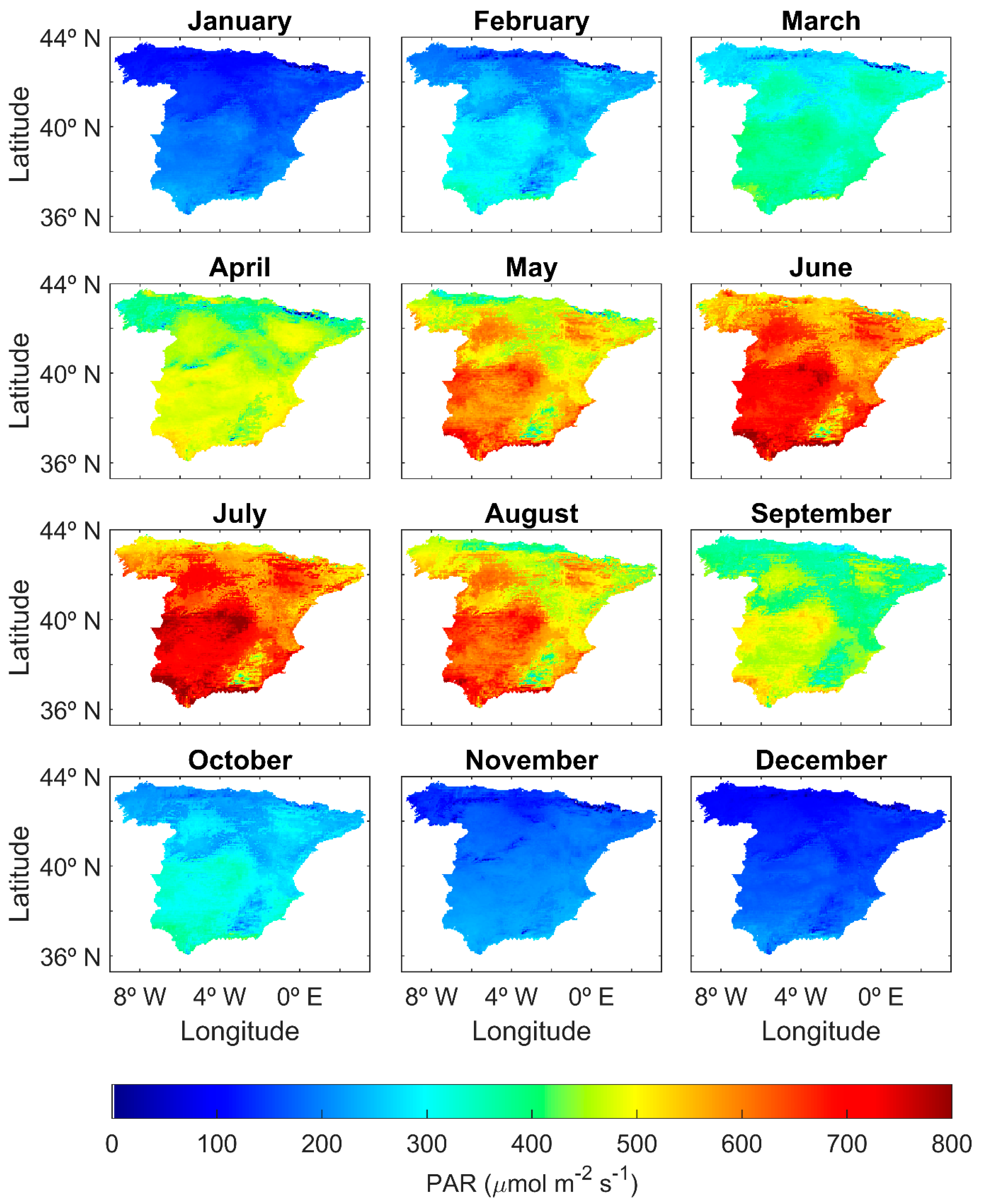
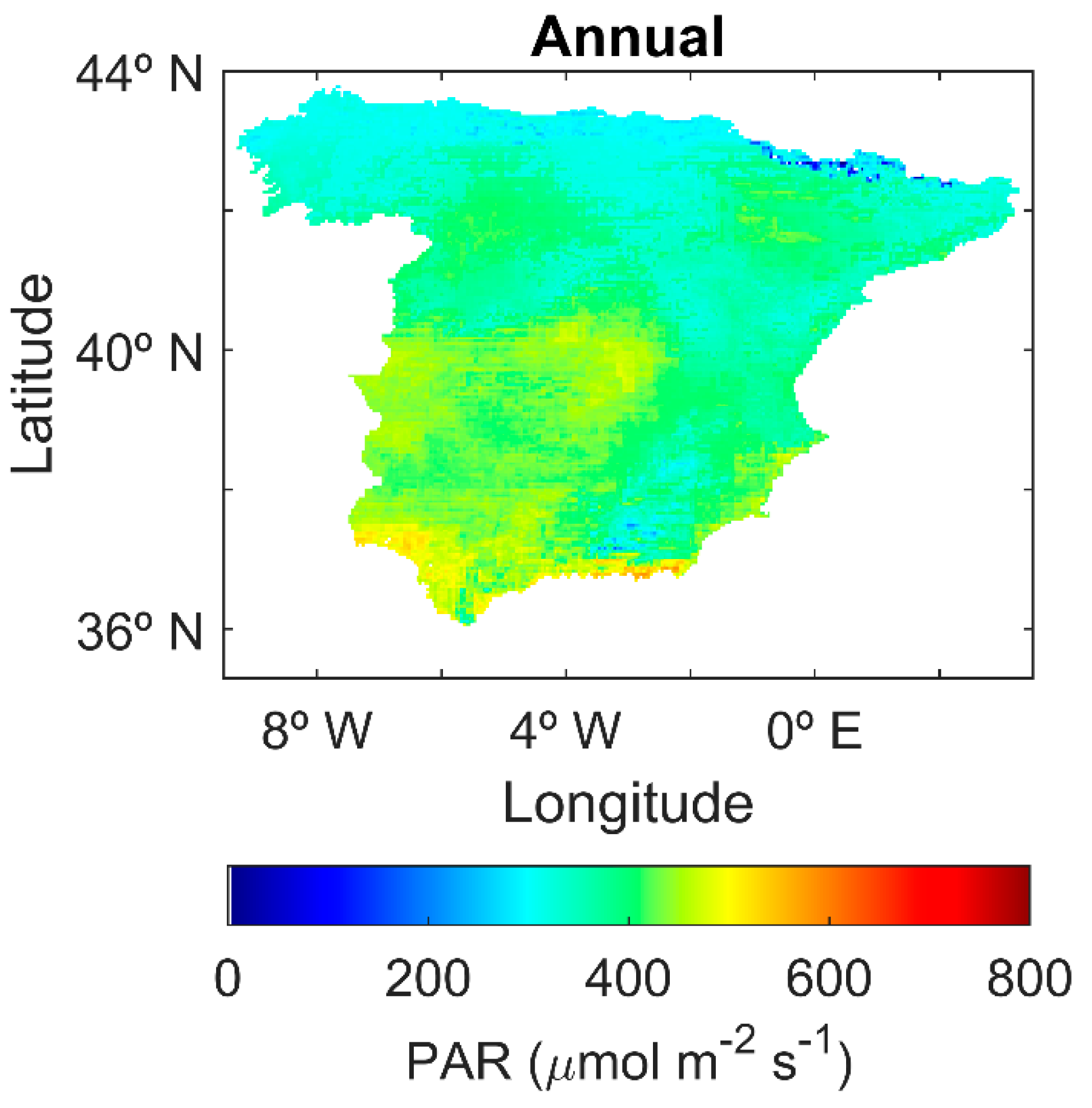
3. Results
Developing PAR Maps
4. Discussion
5. Conclusions
Author Contributions
Funding
Data Availability Statement
Acknowledgments
Conflicts of Interest
References
- McCree, K.J. Test of current definitions of photosynthetically active radiation against leaf photosynthesis data. Agric. Meteorol 1972, 10, 443–453. [Google Scholar] [CrossRef]
- Ross, J.; Sulev, M. Sources of error in measurements of PAR. Agric. For. Meteorol 2000, 100, 103–125. [Google Scholar] [CrossRef]
- Wu, C.; Niu, Z.; Tang, Q.; Huang, W.; Rivard, B.; Feng, J. Remote estimation of gross primary production in wheat using chlorophyll-related vegetation indices. Agric. For. Meteorol 2009, 149, 1015–1021. [Google Scholar] [CrossRef]
- Pinker, R.T.; Zhao, M.; Wang, H.; Wood, E.F. Impact of satellite based PAR on estimates of terrestrial net primary productivity. Int. J. Remote Sens. 2010, 31, 5221–5237. [Google Scholar] [CrossRef]
- Hindersin, S.; Leupold, M.; Kerner, M.; Hanelt, D. Key parameters for outdoor biomass production of Scenedesmus obliquus in solar tracked photobioreactors. J. Appl. Phycol. 2014, 26, 2315–2325. [Google Scholar] [CrossRef]
- Raymond Hunt, E., Jr. Relationship between woody biomass and PAR conversion efficiency for estimating net primary production from NDVI. Int. J. Remote Sens. 1994, 15, 1725–1729. [Google Scholar] [CrossRef]
- Ramírez-Pérez, L.J.; Morales-Díaz, A.B.; De Alba-Romenus, K.; González-Morales, S.; Benavides-Mendoza, A.; Juárez-Maldonado, A. Determination of micronutrient accumulation in greenhouse cucumber crop using a modeling approach. Agronomy 2017, 7, 79. [Google Scholar] [CrossRef]
- Kim, T.H.; Lee, Y.; Han, S.H.; Hwang, S.J. The effects of wavelength and wavelength mixing ratios on microalgae growth and nitrogen, phosphorus removal using Scenedesmus sp. for wastewater treatment. Bioresour. Technol 2013, 130, 75–80. [Google Scholar] [CrossRef]
- Trofimchuk, O.A.; Petikar, P.V.; Turanov, S.B.; Romanenko, S.A. The influence of PAR irradiance on yield growth of Chlorella microalgae. IOP Conf. Ser. Mater. Sci. Eng. 2019, 510. Available online: https://iopscience.iop.org/article/10.1088/1757-899X/510/1/012017/meta (accessed on 25 November 2020). [CrossRef]
- Schmidt, J.J.; Gagnon, G.A.; Jamieson, R.C. Microalgae growth and phosphorus uptake in wastewater under simulated cold region conditions. Ecol. Eng. 2016, 95, 588–593. [Google Scholar] [CrossRef]
- Vadiveloo, A.; Moheimani, N.R.; Cosgrove, J.J.; Bahri, P.A.; Parlevliet, D. Effect of different light spectra on the growth and productivity of acclimated Nannochloropsis sp. (Eustigmatophyceae). Algal. Res. 2015, 8, 121–127. [Google Scholar] [CrossRef]
- Cemek, B.; Demir, Y.; Uzun, S.; Ceyhan, V. The effects of different greenhouse covering materials on energy requirement, growth and yield of aubergine. Energy 2006, 31, 1780–1788. [Google Scholar] [CrossRef]
- Lee, C.S.; Hoes, P.; Cóstola, D.; Hensen, J.L.M. Assessing the performance potential of climate adaptive greenhouse shells. Energy 2019, 175, 534–545. [Google Scholar] [CrossRef]
- Kato, S.; Ackerman, T.P.; Mather, J.H.; Clothiaux, E.E. The k-distribution method and correlated-k approximation for a shortwave radiative transfer model. J. Quant. Spectrosc. Radiat. Transf. 1999, 62, 109–121. [Google Scholar] [CrossRef]
- Wandji Nyamsi, W.; Espinar, B.; Blanc, P.; Wald, L. Estimating the photosynthetically active radiation under clear skies by means of a new approach. Adv. Sci. Res. 2015, 12, 5–10. [Google Scholar] [CrossRef]
- Vindel, J.M.; Valenzuela, R.X.; Navarro, A.A.; Zarzalejo, L.F.; Paz-Gallardo, A.; Souto, J.; Méndez-Gómez, R.; Cartelle, D.; Casares, J. Modeling photosynthetically active radiation from satellite-derived estimations over mainland Spain. Remote Sens. 2018, 10, 849. [Google Scholar] [CrossRef]
- Ferrera-Cobos, F.; Vindel, J.M.; Valenzuela, R.X.; González, J.A. Analysis of spatial and temporal variability of the PAR/GHI ratio and PAR modeling based on two satellite estimates. Remote Sens. 2020, 12, 1262. [Google Scholar] [CrossRef]
- Ferrera-Cobos, F.; Vindel, J.M.; Valenzuela, R.X.; González, J.A. Models for estimating daily photosynthetically active radiation in oceanic and mediterranean climates and their improvement by site adaptation techniques. Adv. Space Res. 2020, 65, 1894–1909. [Google Scholar] [CrossRef]
- Ferrera-Cobos, F.; Vindel, J.M.; Valenzuela, R.X. A New index assessing the viability of par application projects used to validate PAR models. Agronomy 2021, 11, 470. [Google Scholar] [CrossRef]
- Escobedo, J.F.; Gomes, E.N.; Oliveira, A.P.; Soares, J. Modeling hourly and daily fractions of UV, PAR and NIR to global solar radiation under various sky conditions at Botucatu, Brazil. Appl. Energy 2009, 86, 299–309. [Google Scholar] [CrossRef]
- Alados, I.; Foyo-Moreno, I.; Alados-Arboledas, L. Photosynthetically active radiation: Measurements and modelling. Agric. For. Meteorol. 1996, 78, 121–131. [Google Scholar] [CrossRef]
- Janjai, S.; Wattan, R.; Sripradit, A. Modeling the ratio of photosynthetically active radiation to broadband global solar radiation using ground and satellite-based data in the tropics. Adv. Space Res. 2015, 56, 2356–2364. [Google Scholar] [CrossRef]
- Mizoguchi, Y.; Yasuda, Y.; Ohtani, Y.; Watanabe, T.; Kominami, Y.; Yamanoi, K. A practical model to estimate photosynthetically active radiation using general meteorological elements in a temperate humid area and comparison among models. Theor. Appl. Climatol. 2014, 115, 583–589. [Google Scholar] [CrossRef]
- Jacovides, C.P.; Boland, J.; Asimakopoulos, D.N.; Kaltsounides, N.A. Comparing diffuse radiation models with one predictor for partitioning incident PAR radiation into its diffuse component in the eastern Mediterranean basin. Renew. Energy 2010, 35, 1820–1827. [Google Scholar] [CrossRef]
- Pashiardis, S.; Sa, K.; Pelengaris, A. Characteristics of photosynthetic active radiation (PAR) through statistical analysis at Larnaca, Cyprus. SM J. Biom. Biostat. 2017, 2, 1–16. [Google Scholar]
- Yu, X.; Guo, X. Hourly photosynthetically active radiation estimation in Midwestern United States from artificial neural networks and conventional regressions models. Int. J. Biometeorol. 2016, 60, 1247–1259. [Google Scholar] [CrossRef]
- Yu, X.; Wu, Z.; Jiang, W.; Guo, X. Predicting daily photosynthetically active radiation from global solar radiation in the Contiguous United States. Energy Convers. Manag. 2015, 89, 71–82. [Google Scholar] [CrossRef]
- Ren, X.; He, H.; Zhang, L.; Yu, G. Estimation of diffuse photosynthetically active radiation and the spatiotemporal variation analysis in China from 1981 to 2010. J. Geogr. Sci. 2014, 24, 579–592. [Google Scholar] [CrossRef][Green Version]
- Ren, X.; He, H.; Zhang, L.; Yu, G. Global radiation, photosynthetically active radiation, and the diffuse component dataset of China, 1981-2010. Earth Syst. Sci. Data 2018, 10, 1217–1226. [Google Scholar] [CrossRef]
- McCandless, T.C.; Haupt, S.E.; Young, G.S. A model tree approach to forecasting solar irradiance variability. Sol. Energy 2015, 120, 514–524. [Google Scholar] [CrossRef]
- Hu, B.; Wang, Y.; Liu, G. Spatiotemporal characteristics of photosynthetically active radiation in China. J. Geophys. Res. 2007, 112, D14106. [Google Scholar] [CrossRef]
- Pozo-Vázquez, D.; Wilbert, S.; Gueymard, C.; Alados-Arboledas, L.; Santos-Alamillos, F.; Granados-Munoz, M. Interannual variability of long time series of DNI and GHI at PSA, Spain. Proc. SolarPACES Conf. 2011, 1–8. Available online: https://www.researchgate.net/publication/225023716_Interannual_Variability_of_long_time_series_of_DNI_and_GHI_at_PSA_Spain (accessed on 25 May 2018).
- Xia, X.; Li, Z.; Wang, P.; Chen, H.; Cribb, M. Estimation of aerosol effects on surface irradiance based on measurements and radiative transfer model simulations in northern China. J. Geophys. Res. 2007, 112, D22S10. [Google Scholar] [CrossRef]
- Ångström, A. On the atmospheric transmission of sun radiation and on dust in the air. Geogr. Ann. 1929, 11, 156. [Google Scholar] [CrossRef]
- Kidder, S.Q.; Vonder Haar, T.H. Satellite Meteorology—An introduction; Academic Press: Cambridge, MA, USA, 1995; ISBN 978-0124064300. [Google Scholar]
- Alados-Arboledas, L.; Olmo, F.J.; Alados, I.; Pérez, M. Parametric models to estimate photosynthetically active radiation in Spain. Agric. For. Meteorol. 2000, 101, 187–201. [Google Scholar] [CrossRef]
- Foyo-Moreno, I.; Alados, I.; Alados-Arboledas, L. A new conventional regression model to estimate hourly photosynthetic photon flux density under all sky conditions. Int. J. Climatol. 2017, 37, 1067–1075. [Google Scholar] [CrossRef]
- Köppen, W.; Geiger, R. Das geographische system der klimate. In Handbuch der Klimatologie; Gebrüder Bornträger: Berlín, Germany, 1936; p. 44. [Google Scholar]
- Beck, H.E.; Zimmermann, N.E.; McVicar, T.R.; Vergopolan, N.; Berg, A.; Wood, E.F. Present and future Köppen-Geiger climate classification maps at 1-km resolution. Sci. Data 2018, 5, 180214. [Google Scholar] [CrossRef]
- Peel, M.C.; Finlayson, B.L.; McMahon, T.A. Updated world map of the Köppen-Geiger climate classification. Hydrol. Earth Syst. Sci. 2007, 11, 1633–1644. [Google Scholar] [CrossRef]
- Agencia Estatal de Meteorología (AEMET); Instituto de Meteorologia de Portugal (IM). Iberian Climate Atlas; AEMET-Ministerio de Medio Ambiente y Medio Rural y Marino & Instituto de Meteorologia de Portugal: Madrid, Spain, 2011; ISBN 978-84-7837-079-5. [Google Scholar]
- Müller, R.; Pfeifroth, U.; Träger-Chatterjee, C.; Cremer, R.; Trentmann, J.; Hollmann, R. Surface Solar Radiation Data Set—Heliosat (SARAH)—Edition 1. EUMETSAT Satell. Appl. Facil. Clim. Monit. 2015. Available online: https://wui.cmsaf.eu/safira/action/viewDoiDetails?acronym=SARAH_V001 (accessed on 11 December 2019). [CrossRef]
- Schulz, J.; Albert, P.; Behr, H.-D.; Caprion, D.; Deneke, H.; Dewitte, S.; Dürr, B.; Fuchs, P.; Gratzki, A.; Hechler, P.; et al. Operational climate monitoring from space: The EUMETSAT satellite application facility on climate monitoring (CM-SAF). Atmos. Chem. Phys. 2009, 9, 1687–1709. [Google Scholar] [CrossRef]
- Wang, D. MODIS/Terra+Aqua Surface Radiation Daily/3-Hour L3 Global 5km SIN Grid V006 [Data Set]. Available online: https://lpdaac.usgs.gov/products/mcd18a1v006 (accessed on 10 November 2019). [CrossRef]
- Wang, D. MODIS/Terra+Aqua Photosynthetically Active Radiation Daily/3-Hour L3 Global 5km SIN Grid V006 [Data Set]. Available online: https://lpdaac.usgs.gov/products/mcd18a2v006 (accessed on 10 November 2019). [CrossRef]
- Wang, D.; Liang, S.; Zhang, Y.; Gao, X.; Brown, M.G.L.; Jia, A. A new set of MODIS land products (MCD18): Downward shortwave radiation and photosynthetically active radiation. Remote Sens. 2020, 12, 168. [Google Scholar] [CrossRef]
- Bernardos, A.; Gastón, M.; Fernández-Peruchena, C.; Martín, L.; Bermejo, D.; Vindel, J.M.; Ramírez, L.; Liria, J. Solar Resource Mapping in Tanzania; Solar Modeling Report; World Bank Group: Washington, DC, USA, 2015. [Google Scholar]
- Ferrera Cobos, F. Desarrollo de una Red de Medidas y Modelización de la Radiación Fotosintéticamente Activa; Universidad Politécnica de Madrid: Madrid, Spain, 2021. [Google Scholar] [CrossRef]
- Aguiar, L.J.G.; Fischer, G.R.; Ladle, R.J.; Malhado, A.C.M.; Justino, F.B.; Aguiar, R.G.; da Costa, J.M.N. Modeling the photosynthetically active radiation in South West Amazonia under all sky conditions. Theor. Appl. Climatol. 2012, 108, 631–640. [Google Scholar] [CrossRef]
- Hao, D.; Wen, J.; Xiao, Q.; Wu, S.; Lin, X.; You, D.; Tang, Y. Modeling anisotropic reflectance over composite sloping terrain. IEEE Trans. Geosci. Remote Sens. 2018, 56, 3903–3923. [Google Scholar] [CrossRef]
- Yin, G.; Li, A.; Zhao, W.; Jin, H.; Bian, J.; Wu, S. Modeling canopy reflectance over sloping terrain based on path length correction. IEEE Trans. Geosci. Remote Sens. 2017, 55, 4597–4609. [Google Scholar] [CrossRef]
- Wen, J.; Liu, Q.; Xiao, Q.; Liu, Q.; You, D.; Hao, D.; Wu, S.; Lin, X. Characterizing land surface anisotropic reflectance over rugged terrain: A review of concepts and recent developments. Remote Sens. 2018, 10, 370. [Google Scholar] [CrossRef]


| Station | Altitude (m) | Latitude (°, +N) | Longitude (°, +E) | Climate |
|---|---|---|---|---|
| Álava-NEIKER | 520 | 42.85 | −2.62 | oceanic |
| Albacete-ITAP | 698 | 39.04 | −2.08 | Mediterranean |
| Asturias-SERIDA | 6 | 43.48 | −5.44 | oceanic |
| Córdoba-IFAPA | 91 | 37.86 | −4.80 | Mediterranean |
| Lugo-USC | 447 | 43.00 | −7.54 | oceanic |
| Salamanca-CIALE | 777 | 40.98 | −5.72 | Mediterranean |
| Zaragoza-Aula Dei | 226 | 41.73 | −0.81 | Mediterranean |
| Station | Number of Original Recordings | Number of Recordings after Filtering |
|---|---|---|
| Álava-NEIKER | 785 | 784 |
| Albacete-ITAP | 785 | 783 |
| Asturias-SERIDA | 784 | 779 |
| Córdoba-IFAPA | 785 | 784 |
| Lugo-USC | 785 | 769 |
| Salamanca-CIALE | 785 | 785 |
| Zaragoza-Aula Dei | 785 | 782 |
| Station | a | b | c (μmol m−2 s−1) |
|---|---|---|---|
| Álava-NEIKER | 0.26 | 0.79 | −9.58 |
| Albacete-ITAP | −0.25 | 1.36 | −18.46 |
| Asturias-SERIDA | −0.41 | 1.54 | −20.41 |
| Córdoba-IFAPA | −0.09 | 1.18 | −13.89 |
| Lugo-USC | 1.24 | −0.27 | −0.71 |
| Salamanca-CIALE | 0.34 | 0.66 | −8.02 |
| Zaragoza-Aula Dei | 0.29 | 0.79 | −9.77 |
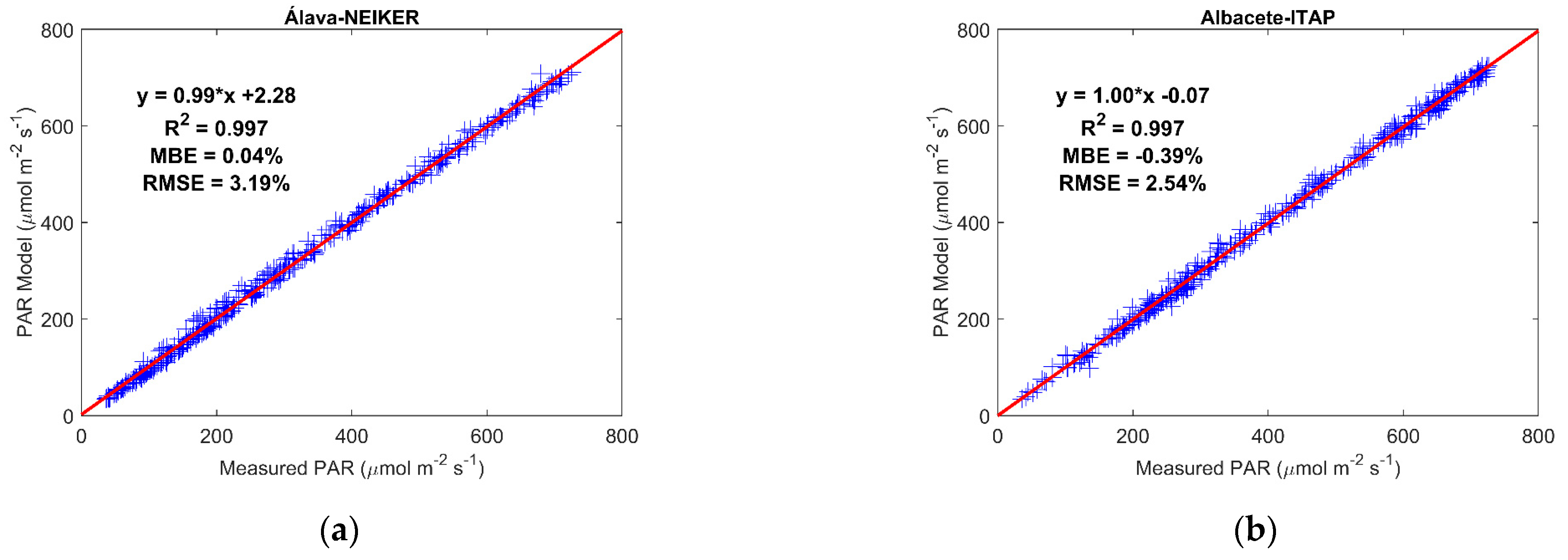
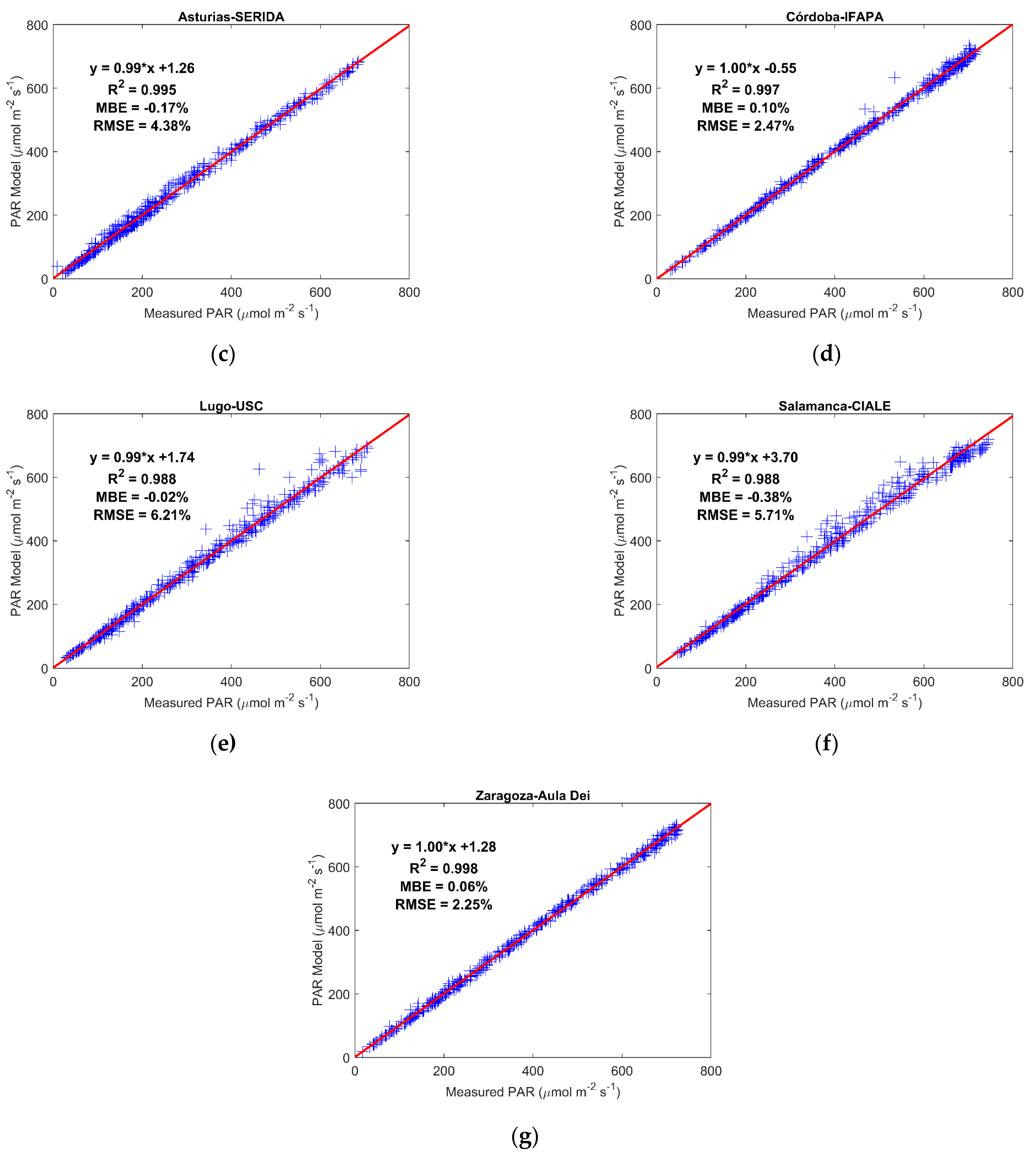
| Álava-NEIKER | Albacete-ITAP | Asturias-SERIDA | Córdoba-IFAPA | Lugo-USC | Salamanca-CIALE | Zaragoza-Aula Dei | ||
|---|---|---|---|---|---|---|---|---|
| PAR model | Slope | 0.99 | 1.00 | 0.99 | 1.00 | 0.99 | 0.99 | 1.00 |
| Intercept | 2.28 | −0.07 | 1.26 | −0.55 | 1.74 | 3.70 | 1.28 | |
| R2 | 0.997 | 0.997 | 0.995 | 0.997 | 0.988 | 0.988 | 0.998 | |
| MBE | 0.04 | −0.39 | −0.17 | 0.10 | −0.02 | −0.38 | 0.06 | |
| RMSE | 3.19 | 2.54 | 4.38 | 2.47 | 6.21 | 5.71 | 2.25 |
| Álava-NEIKER | Albacete-ITAP | Asturias-SERIDA | Córdoba-IFAPA | Lugo-USC | Salamanca-CIALE | Zaragoza-Aula Dei | ||
|---|---|---|---|---|---|---|---|---|
| CM-SAF model | Slope | 0.93 | 0.92 | 0.91 | 0.93 | 0.94 | 0.96 | 0.89 |
| Intercept | 13.23 | 13.72 | 16.05 | 12.13 | 15.84 | 16.77 | 13.22 | |
| R2 | 0.997 | 0.997 | 0.995 | 0.997 | 0.987 | 0.987 | 0.998 | |
| MBE | 3.16 | 4.72 | 3.82 | 4.34 | 1.45 | 0.13 | 7.45 | |
| RMSE | 6.07 | 6.46 | 8.15 | 5.90 | 7.59 | 5.99 | 9.43 | |
| MODIS model | Slope | 1.02 | 1.01 | 0.96 | 1.02 | 1.01 | 1.04 | 0.99 |
| Intercept | 2.99 | −1.60 | 6.81 | 0.71 | 6.30 | 4.14 | 1.19 | |
| R2 | 0.997 | 0.996 | 0.994 | 0.997 | 0.988 | 0.987 | 0.998 | |
| MBE | −2.75 | −0.25 | 1.32 | −1.91 | −2.83 | −4.63 | 0.58 | |
| RMSE | 4.52 | 3.11 | 5.46 | 3.40 | 7.19 | 7.87 | 2.52 | |
| Escobedo et al., 2009 model | Slope | 1.11 | 1.10 | 1.07 | 1.10 | 1.10 | 1.13 | 1.06 |
| Intercept | 3.77 | 4.96 | 4.07 | 5.80 | 6.49 | 10.93 | 8.13 | |
| R2 | 0.998 | 0.998 | 0.999 | 0.996 | 0.989 | 0.987 | 0.998 | |
| MBE | 12.18 | 10.87 | 8.38 | 11.10 | 12.32 | 16.02 | 8.32 | |
| RMSE | 14.12 | 11.96 | 9.79 | 12.31 | 15.64 | 18.60 | 9.26 | |
| Aguiar et al., 2012 pasture model | Slope | 1.00 | 0.98 | 0.97 | 0.99 | 0.99 | 1.02 | 0.96 |
| Intercept | 31.81 | 35.05 | 31.96 | 34.60 | 35.83 | 38.17 | 36.25 | |
| R2 | 0.998 | 0.998 | 0.999 | 0.996 | 0.987 | 0.986 | 0.998 | |
| MBE | 9.96 | 6.76 | 8.09 | 6.87 | 10.37 | 12.04 | 4.94 | |
| RMSE | 10.30 | 7.08 | 8.62 | 7.45 | 12.42 | 13.51 | 5.82 | |
| Aguiar et al., 2012 forest model | Slope | 0.95 | 0.94 | 0.92 | 0.94 | 0.94 | 0.98 | 0.91 |
| Intercept | 6.79 | 9.73 | 7.00 | 8.97 | 9.69 | 11.89 | 10.17 | |
| R2 | 0.998 | 0.998 | 0.999 | 0.996 | 0.986 | 0.987 | 0.998 | |
| MBE | −2.63 | −4.17 | −5.59 | −3.89 | −2.80 | 0.57 | −5.91 | |
| RMSE | 4.64 | 5.41 | 7.86 | 5.32 | 8.15 | 5.91 | 7.67 | |
| New model | Slope | 0.99 | 1.00 | 0.99 | 1.00 | 0.99 | 0.99 | 1.00 |
| Intercept | 2.28 | −0.07 | 1.26 | −0.55 | 1.74 | 3.70 | 1.28 | |
| R2 | 0.997 | 0.997 | 0.995 | 0.997 | 0.988 | 0.988 | 0.998 | |
| MBE | 0.04 | −0.39 | −0.17 | 0.10 | −0.02 | −0.38 | 0.06 | |
| RMSE | 3.19 | 2.54 | 4.38 | 2.47 | 6.21 | 5.71 | 2.25 |
Publisher’s Note: MDPI stays neutral with regard to jurisdictional claims in published maps and institutional affiliations. |
© 2021 by the authors. Licensee MDPI, Basel, Switzerland. This article is an open access article distributed under the terms and conditions of the Creative Commons Attribution (CC BY) license (https://creativecommons.org/licenses/by/4.0/).
Share and Cite
Ferrera-Cobos, F.; Vindel, J.M.; Wane, O.; Navarro, A.A.; Zarzalejo, L.F.; Valenzuela, R.X. Combination of Models to Generate the First PAR Maps for Spain. Remote Sens. 2021, 13, 4950. https://doi.org/10.3390/rs13234950
Ferrera-Cobos F, Vindel JM, Wane O, Navarro AA, Zarzalejo LF, Valenzuela RX. Combination of Models to Generate the First PAR Maps for Spain. Remote Sensing. 2021; 13(23):4950. https://doi.org/10.3390/rs13234950
Chicago/Turabian StyleFerrera-Cobos, Francisco, Jose M. Vindel, Ousmane Wane, Ana A. Navarro, Luis F. Zarzalejo, and Rita X. Valenzuela. 2021. "Combination of Models to Generate the First PAR Maps for Spain" Remote Sensing 13, no. 23: 4950. https://doi.org/10.3390/rs13234950
APA StyleFerrera-Cobos, F., Vindel, J. M., Wane, O., Navarro, A. A., Zarzalejo, L. F., & Valenzuela, R. X. (2021). Combination of Models to Generate the First PAR Maps for Spain. Remote Sensing, 13(23), 4950. https://doi.org/10.3390/rs13234950