Article

Development of Prediction Models for Estimating Key Rice Growth Variables Using Visible and NIR Images from Unmanned Aerial Systems

1
The State Key Laboratory of Soil and Sustainable Agriculture, Institute of Soil Science Chinese Academy of Sciences, Nanjing 210008, China
2
College of Advanced Agricultural Sciences, University of Chinese Academy of Sciences, Beijing 100049, China
*
Author to whom correspondence should be addressed.
Remote Sens. 2022, 14(6), 1384; https://doi.org/10.3390/rs14061384
Submission received: 11 January 2022 / Revised: 6 March 2022 / Accepted: 8 March 2022 / Published: 13 March 2022
(This article belongs to the Special Issue Remote Sensing of Agro-Ecosystems)

Abstract

:
The rapid and accurate acquisition of rice growth variables using unmanned aerial system (UAS) is useful for assessing rice growth and variable fertilization in precision agriculture. In this study, rice plant height (PH), leaf area index (LAI), aboveground biomass (AGB), and nitrogen nutrient index (NNI) were obtained for different growth periods in field experiments with different nitrogen (N) treatments from 2019–2020. Known spectral indices derived from the visible and NIR images and key rice growth variables measured in the field at different growth periods were used to build a prediction model using the random forest (RF) algorithm. The results showed that the different N fertilizer applications resulted in significant differences in rice growth variables; the correlation coefficients of PH and LAI with visible-near infrared (V-NIR) images at different growth periods were larger than those with visible (V) images while the reverse was true for AGB and NNI. RF models for estimating key rice growth variables were established using V-NIR images and V images, and the results were validated with an R2 value greater than 0.8 for all growth stages. The accuracy of the RF model established from V images was slightly higher than that established from V-NIR images. The RF models were further tested using V images from 2019: R2 values of 0.75, 0.75, 0.72, and 0.68 and RMSE values of 11.68, 1.58, 3.74, and 0.13 were achieved for PH, LAI, AGB, and NNI, respectively, demonstrating that RGB UAS achieved the same performance as multispectral UAS for monitoring rice growth.

1. Introduction

Rice is one of the most important crops worldwide and plays an important role in food security [1]. Rapid and accurate monitoring of key rice growth variables is important for rice fertilizer management [2,3]. Precision fertilization improves the fertilizer utilization rate and rice yield and reduces environmental pollution [4].
Rice growth variables, such as plant height (PH), leaf area index (LAI), and aboveground biomass (AGB), are often used to diagnose crop growth in agricultural management practices [5]. The nitrogen nutrient index (NNI) is a key indicator that can accurately reflect the N nutrition status of different crops and is relatively stable in diagnosing N nutrition status [6,7]. The most accurate method of obtaining values for these variables is destructive sampling followed by laboratory measurements; however, this is labor-intensive and time-consuming [8,9]. Therefore, handheld instruments for obtaining crop growth variables have been developed in recent years. As a result, handheld instruments started to be used for in situ measuring crop growth variables. A common example are chlorophyll meters, which was used to predict leaf nitrogen content from reflectance measurements in the visual and near-infrared spectrum [10]. Digital images were used to obtain crop canopy cover and a new method of NNI acquisition was established using canopy cover instead of dry crop biomass [11]. However, these methods cannot obtain crop growth variables within the entire field in real time, which has some limitations in precision agriculture guidance.
In recent decades, satellite remote sensing has been used to monitor crop AGB [12,13], LAI [14,15,16], N content [17], and yield [18]. Different vegetation indexes (VIs) have been extracted from satellite imagery to estimate key growth variables by modeling their relationships [19]. Although satellite imagery has achieved fast and accurate monitoring of crop growth in large fields, it is still difficult to use at the field scale because of limitations in the image resolutions [20]. Therefore, there is an urgent need for a method for acquiring high-resolution remote sensing images to monitor crop growth variables at the field scale. With the advancement of sensing technologies, unmanned aerial system (UAS) has been increasingly used in precision agriculture [21]. UAS has been used to monitor crop growth by acquiring high spatial resolution image data and has received more attention for field-scale crop monitoring than satellite remote sensing due to their practicality and low cost [22,23].
UAS can carry different camera sensors, including RGB [24], multispectral [25], hyperspectral [26], and thermal infrared [27] cameras. Images captured by different cameras can be processed to extract multiple VIs, select sensitive bands, and extract image texture information [28]. Real-time and accurate estimation of crop growth variables can be achieved by establishing estimation models between image information and crop growth variables [29]. Past studies have extracted spectral information from hyperspectral images by UAS, enabling crop phenotype diagnosis [30], nutritional status determination [26], and yield estimation [31]. Hyperspectral images contain abundant and continuous spectral information and provide rich information about crop physiological variables. Therefore, studies have been conducted to monitor crop growth and nutritional status using multispectral cameras [28,32]. However, their high cost and the complexity of processing their information limit their widespread application in agriculture.
Studies have been conducted from the perspective of model algorithms to improve the accuracy of UAS imagery for monitoring crop growth variables. A single VI, such as the normalized vegetation index (NDVI), obtained by combining red and near-infrared bands, uses limited band information. To make full use of the information in each band of the image, multiple VIs need to be combined to predict crop growth variables [33,34]. Machine learning algorithms present a scalable, modular strategy for data analysis that can combine large amounts of raw spectral band and VI information and then extract the best band information or VI with the crop growth variables for modeling. Machine learning algorithms have been frequently used in recent years in remote sensing to monitor crop growth indicators [35]. For example, Gahrouei et al. (2020) evaluated the potential of RapidEye imagery data in estimating biomass and LAI using a machine learning algorithm and demonstrated that the support vector machine algorithm was more accurate than the artificial neural network algorithm [36]. Wang et al. developed a model using multiple VIs to estimate winter wheat biomass with a random forest (RF) machine learning model and found that it performed better than artificial neural network and support vector regression models [37].
Although there have been many studies on sensor types, image processing methods, and model construction methods using UAS to monitor crop growth variables and yield estimation, the difference in accuracy between V-NIR images and V images for estimating rice growth variables remains unclear.
In this study, we compare the features of V-NIR images and V images from UAS by obtaining VIs from the two kinds of images and comparing their relationships with PH, LAI, AGB, and NNI. Then the accuracy of machine learning models will be validated to estimate PH, LAI, AGB, and NNI. The objectives of this study are (1) to analyze the effects of different nitrogen fertilizer applications on rice growth variables at different growth periods; and (2) to find the VIs from the V-NIR images and the V images that better correlate with the studied rice growth variables.

2. Materials and Methods

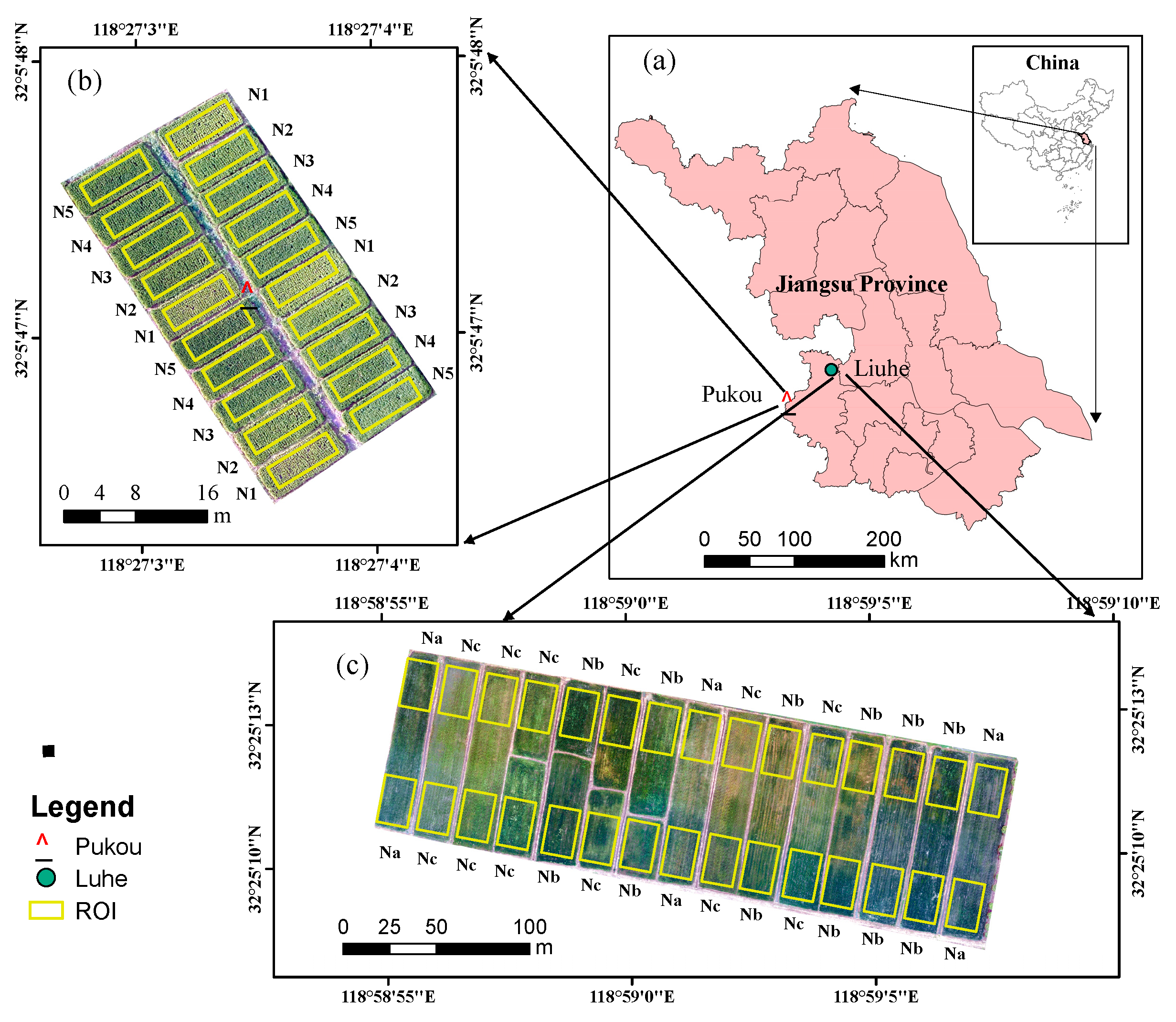
2.1. Experimental Design

Field experiments were conducted in the Pukou and Luhe Districts, Nanjing, Jiangsu Province, China (32°04′15″N, 118°28′21″E and 32°25′4″N, 118°59′18″E, respectively) for two consecutive years (2019–2020) (Figure 1). The experimental region has a tropical humid climate with an average annual temperature of 15.4 °C. Nanjing 5055, a japonica rice cultivar with strong disease resistance, was used in the experiments. In each experimental plot, the planting density was 105 kg ha−1. The cultivation method involved transplanting transplants, which started when the seedlings had about two tillers, and the transplanting interval of seedlings was 20 × 20 cm; the details of the treatments are shown in Table 1 and Figure 1.
Pukou field experiment: The area of this experimental field was 0.27 ha and was divided into 20 plots for five treatments with four replicates (Figure 1 and Table 1). The soil type in the area was paddy soil with 22.26 g kg−1 organic matter, 1.31 g kg−1 total N, 15.41 mg kg−1 Olsen-P, and 146.4 mg kg−1 NH4OAc-K. Rice was transplanted on 12 June 2019, and harvested on 2 November 2019, 20 June 2020, and 10 November 2020.
Luhe field experiment: The area of the experimental field was 3 ha and was divided into 15 plots for three treatments with five replicates (Figure 1 and Table 1). The soil in the Luhe experimental station was a silt loam with 26.56 g kg−1 organic matter, 1.58 g kg−1 total N, 15.21 mg kg−1 Olsen-P, and 166.2 g kg−1 NH4OAc-K. Rice was transplanted on 18 June 2019, and harvested on 5 November 2019, 20 June 2020, and 16 November 2020.

2.2. Measurement of Rice Growth Variables

V images were taken using UAS at the rice jointing, flowering, filling, and maturity stages in 2019 and 2020, whereas V-NIR images were captured only in 2020. In each experimental plot in Pukou, three representative rice plants were collected and processed in the laboratory for analysis. In the Luhe experiment, two samples from one experimental plot were selected and the method was the same as that in the Pukou experimental field. The PH of three rice plants from each sampling site was randomly measured and averaged. The rice stems and leaves of all samples were separated in the laboratory. Fresh leaves of each sample were scanned using a BenQ M209 Pro flatbed scanner (BenQ, Inc.) to obtain scanned images and calculate the LAI by binarizing the images. The aboveground organs of rice were heated at 105 °C for 30 min, dried at 80 °C to a constant weight, weighed to determine the rice aboveground biomass (AGB), and the total N content of the aboveground organs was measured using the Kjeldahl method. The descriptive statistics for PH, AGB, and LAI at different growth stages are shown in Table 2.

2.3. Calculation of Nitrogen Nutrient Index

NNI is the ratio between plant nitrogen concentration and critical N content, which describes the nitrogen status of rice independent of the growth stage. An NNI value of 1 indicates optimum N, while a value greater or smaller than 1 indicates excessive or deficient N, respectively [2]. Table 2 presents the descriptive statistics of the NNI at different stages of rice growth.
The critical N content ( N c ) of rice was described by the following Equation (1) [11]:
N c = 3.33 A G B 0.26
where N c is the critical N content as a percentage of dry biomass and AGB is the dry weight of aboveground biomass in t ha−1.
The NNI was calculated using Equation (2):
N N I = N a N c
where N a is the measured N content.

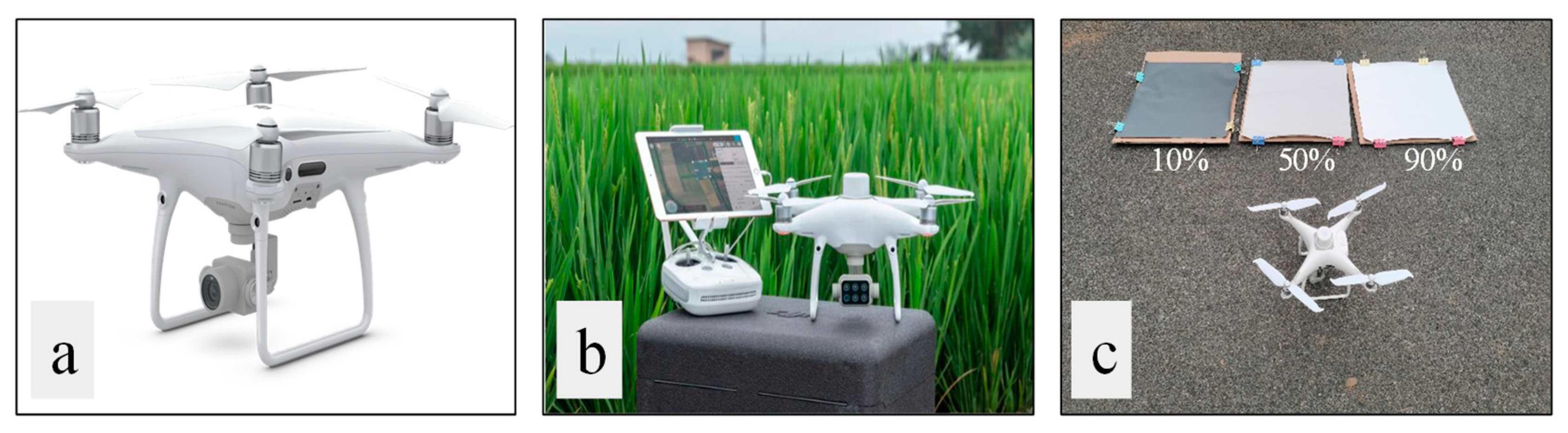
2.4. Acquisition of V Images and V-NIR Images by UAS

A Phantom 4 Professional UAS (SZ DJI Technology Co., Shenzhen, China) carrying a digital camera and multispectral camera was used to acquire high spatial resolution images for each sampling period. The digital camera could take visible light (RGB) photos with 20 million pixels, containing red, green, and blue bands, and the multispectral camera could acquire multispectral photos with 20 million pixels containing red, green, blue, near-infrared, and red-edge bands, which generated TIFF format images with the spatial resolution (pixel size) of 0.03 m. All images were taken by UAS under cloudless, windless, and clear weather conditions from 11:00 to 13:00. The UAS was flown at an altitude of 100 m and speed of 8 m s−1 and the camera was set to shoot automatically at a time interval of 2 s. The side and forward overlap properties of the images were set to 60–80%. Considering reflectivity correction, three diffuse reflective plates (Guangzhou Changhui Electronic Technology Co., Ltd.) (Figure 2c), with reflectivity values of 10%, 50%, and 90%, respectively, were placed on the ground when the UAS was flying.

2.5. Image Processing

Pix4Dmapper (https://www.pix4d.com/; accessed on 20 December 2020) was used to generate orthophotos from acquired images. This process included importing images, aligning them, constructing dense point clouds, constructing grids, generating orthophotos, generating TIFF format images with geographic coordinate systems, and performing grid division using default parameter analysis. Then, for radiometric calibration, calibration boards were used to convert the image value into image reflectivity through the reflectivity measured by the ground target. Python3.7.8 was used to calculate the corresponding VI from the V images and V-NIR images (Table 3). Three rice plants were randomly selected from each plot to represent the sampling points of that plot. ArcGIS10.3 (https://www.esri.com; accessed on 5 January 2021) was used to draw the region of interest (ROI) in the center of each plot and the average values of various VIs at different periods in each ROI were extracted as the VI for each plot.

2.6. Random Forest Algorithm

Machine learning models have been widely used to estimate crop growth variables. Several studies have determined RF to be the best performing and most stable model [55,56]. Therefore, an RF algorithm-based model was developed to estimate the key growth variables of rice. Eleven VIs from V images and nine VIs from V-NIR images (Table 1) were used as input layers and PH, LAI, AGB, and NNI were used as output layers. In the RF model, the number of decision trees was 800, the maximum tree depth was 14, the maximum number of features for the tree was four, and the minimum number of samples required for internal node subdivision was three.

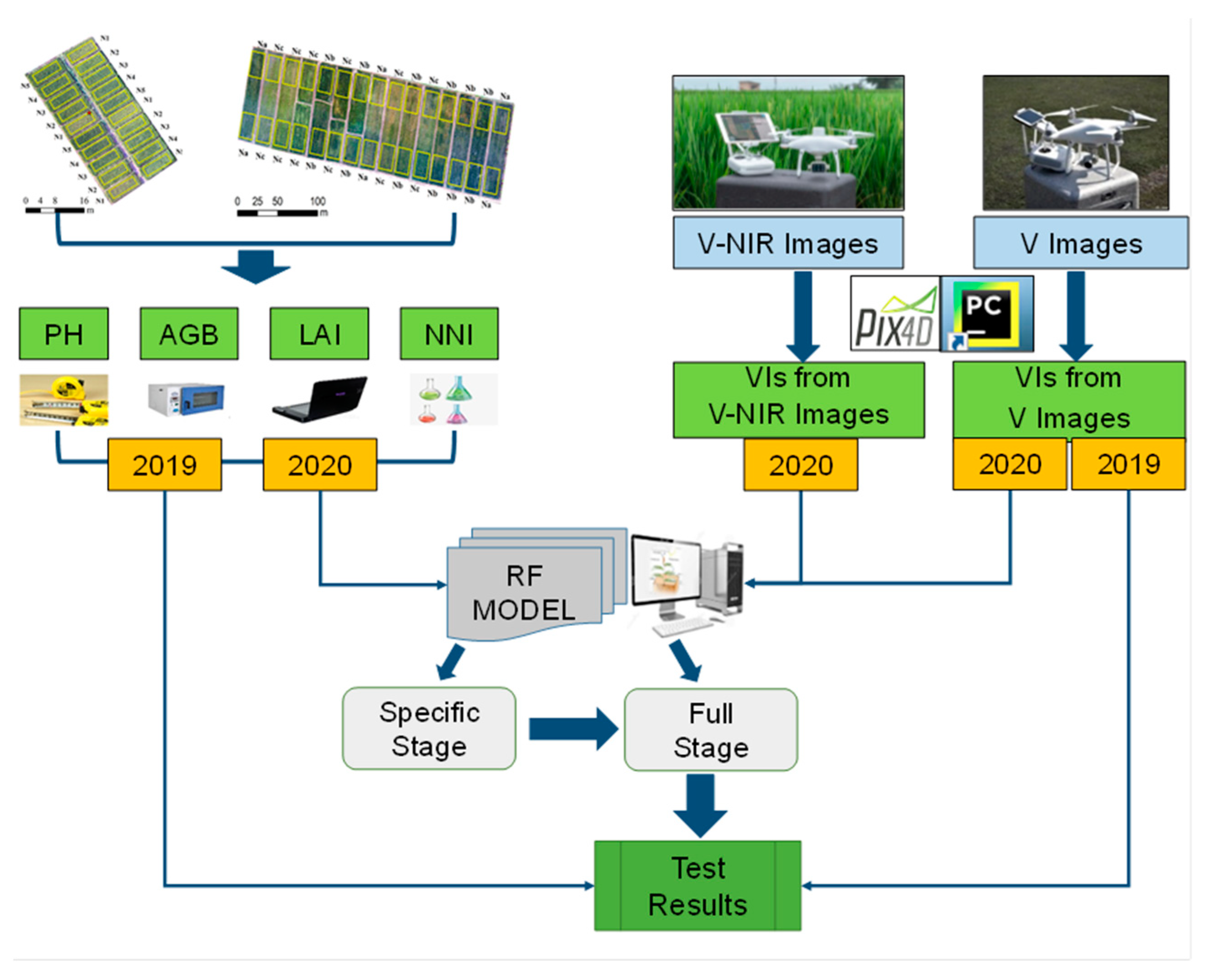
2.7. Model Building and Test

For building the RF model, 70% of the data from 2020 were used for training and the remaining 30% were used for validation. To test the stability of the chosen optimal model algorithm, V images from 2019 were used to predict rice growth variables based on the V images model built for 2020. The coefficient of determination (R2) and root mean square error (RMSE) were calculated to verify the reliability of the model as follows:
R 2 = i = 1 n ( X i X ¯ ) 2 ( Y Y ¯ ) 2 i = 1 n ( X i X ¯ ) 2 i = 1 n ( Y Y ¯ ) 2
R M S E = 1 n i = 1 n ( Y i X i ) 2
where Xi and Yi are the estimated and measured values, respectively; X ¯ and Y ¯ are the average estimated and measured values, respectively; and n is the number of samples.
An overview of this study is presented in Figure 3. First, PH, LAI, AGB, NNI, V images, and V-NIR images were obtained at the jointing, flowering, filling, and maturity stages in 2019 and 2020. Then, estimation models of rice variables were established using the RF algorithm based on the two types of images from UAS for different stages and the entire growth period in 2020. Finally, the model established in 2020 for the entire growth period was tested using experimental data from 2019 to prove its feasibility.

3. Results

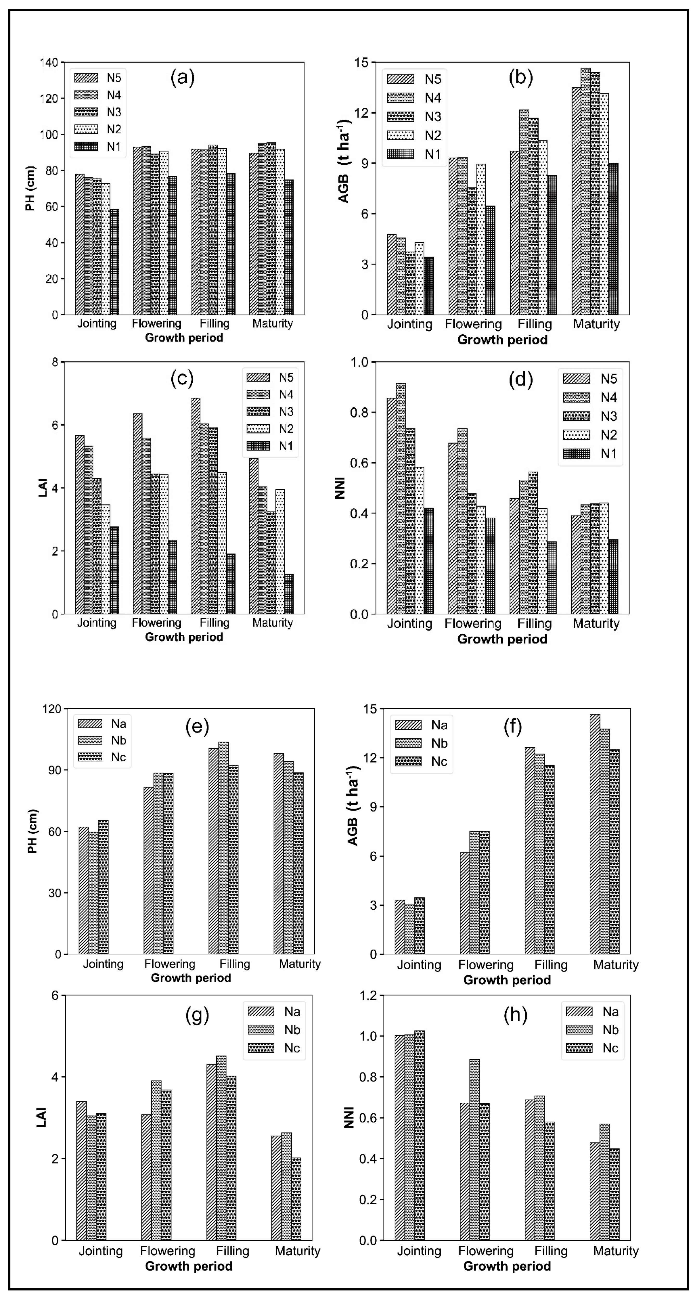
3.1. Effects of Nitrogen Input on Rice Growth Variables

Figure 4 shows histograms of rice growth variables under different N fertilization treatments at different periods in the Pukou and Luhe experiments. These results reflect the status of each growth variable influenced by N fertilization factors and changes in rice growth. The rice variables showed different characteristics under different fertilization treatments during the same growth period. In the Pukou experiment, the pH in the N5, N4, N3, and N2 treatments was equal in each growth period; however, the pH for each growth period was lower in the N1 treatment. Similarly, in the Luhe experiment, the PH in the Nb and Na treatments was approximately equal and slightly higher than that in the Nc treatment for each growth period, which indicated that the same amount of N was applied and the controlled-release fertilizer and conventional fertilizer treatments had little effect on the PH. Reduced N fertilization or no fertilization would lower the PH and impact rice growth.
In Pukou, the AGB was highest in the N5 and N4 treatments at the jointing and flowering stages, followed by N2, N4, and N3. As rice growth proceeded, AGB became the highest in the N4 treatment, followed by N3. Throughout the growth period, AGB was the lowest in the N1 treatment. In the Luhe experiment, throughout the growth period, the AGB was the highest in the Nb treatment, followed by Na, and then Nc, which indicated that the nitrogen reduction treatment or no fertilizer application affected the AGB.
LAI first showed an increasing trend as the growth period progressed, peaking at the filling period, and then gradually decreasing, probably due to increased yellow and withered leaves at maturity. From the jointing to the filling periods, a greater proportion of controlled-release N fertilizer resulted in a greater LAI value, showing a trend of N5 > N4 > N3 > N2 > N1. In the Luhe experiment, the LAI of the Nc-treated field was larger than that of the Nb-treated field during the jointing period. During the flowering period, the LAI of the Na-treated field was smaller than that of the Nb-treated field, probably due to the incomplete release of controlled-release N at the jointing. During the flowering period, the nitrogen from the controlled-release fertilizer treatment was released continuously, and the conventional fertilizer application showed insufficient nitrogen; therefore, the LAI under the conventional fertilizer treatment was smaller than that under the controlled-release fertilizer treatment.
In the Pukou experiment, throughout the growth period, the NNI was higher in the N5, N4, and N3 treatments than in the N2 and N1 treatments, with the NNI in N1 always the lowest. In the Luhe experiment, the NNI in the three fertilizer treatments was approximately equal during the jointing period. However, as rice growth proceeded, the NNI in Nb treatment became greater than those in Na and Nc, which indicated that the amount of N fertilizer applied and the release efficiency of N fertilizer impacted the NNI. Overall, the results of this study indicate that different N applications resulted in significant variability in rice growth variables over different growth periods.

3.2. Correlation between Rice Growth Variables and VIs from V Images and V-NIR Images

Linear correlation analysis of the rice growth variables was performed using VI from V images and V-NIR images for each period (Table 4). The linear correlation coefficients of PH and LAI with VI from V-NIR images were higher than those with VI from V images throughout the entire growth period, indicating that V-NIR images were better for monitoring PH and LAI when using a simple linear model. For AGB and NNI, the correlation coefficients of the measured data with VI from V images were better than those with VI from V-NIR images throughout the growth period.
However, the optimal VIs from images differed for each measured variable at different growth periods and it was difficult to select the VIs for practical applications. The correlation coefficients of some VIs from images with the measured variables were relatively poor: the correlation coefficient of PH with RVI was 0.3 at the maturity period and that of AGB with ExB was 0.2 at the flowering period, meaning they were not conducive to the estimation of the rice growth variable. Therefore, a method is needed to integrate the optimal VI from images with the measured rice variables to establish an estimation model for predicting rice growth variables.

3.3. RF Models Validation for Rice Growth Variable Estimation per Growth Stage

An RF model was built to estimate rice growth variables with VI from V-NIR images and V images for different periods and the results are shown in Figure 5. For PH, the estimation using VI from V-NIR images was the best; however, for AGB, LAI, and NNI, VI from V images obtained the best results. The validation accuracy exceeded 0.8 for the estimations of all growth variables, which demonstrated that the estimation accuracy of rice growth variables could be improved by using the RF algorithm combined with images from UAS, and that V images and V-NIR images both performed well in estimating rice growth variables in different growth periods.

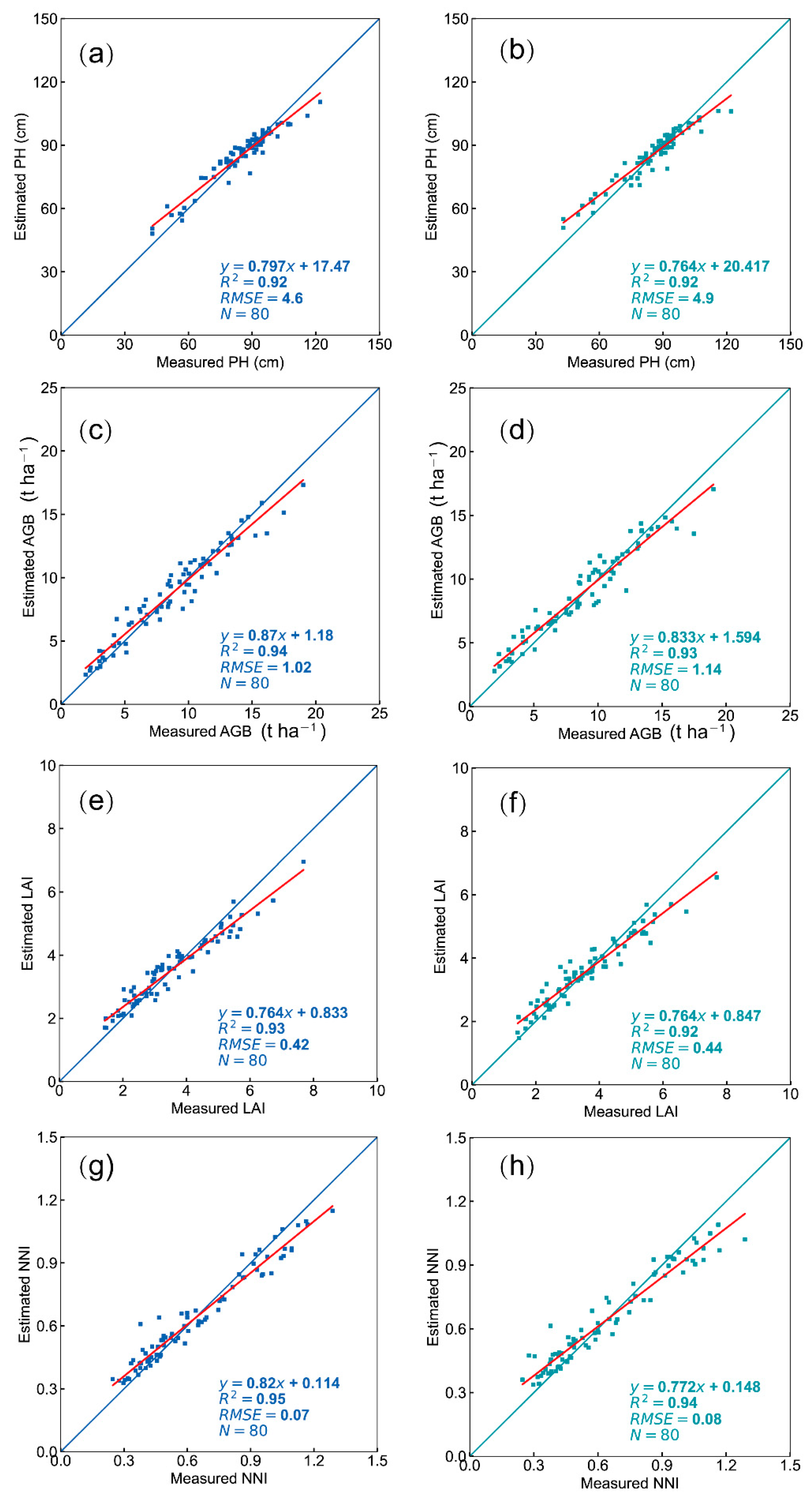
3.4. RF Models Validation for Rice Growth Variable Estimation in Full Stage

Rice growth variables and VI from V images and V-NIR images at the jointing, flowering, filling, and maturity periods were measured in the two experimental areas and integrated to form a database of multiperiod VIs. The RF models were built separately using different rice growth variables with VI from V images and V-NIR images, and the validations are shown in Figure 6. The R2 of the RF model using either VI from V images or VI from V-NIR images for each rice growth variable was greater than 0.9, indicating that the estimations were well achieved using both image types. For the estimations of PH, LAI, AGB, and NNI, the validation accuracy using VI from V images was slightly higher than that obtained using VI from V-NIR images.
Overall, the RF models using V images and V-NIR images from UAS both achieved good results. However, as V images are much cheaper than V-NIR images, the RF model established based on V images is better for monitoring rice growth.

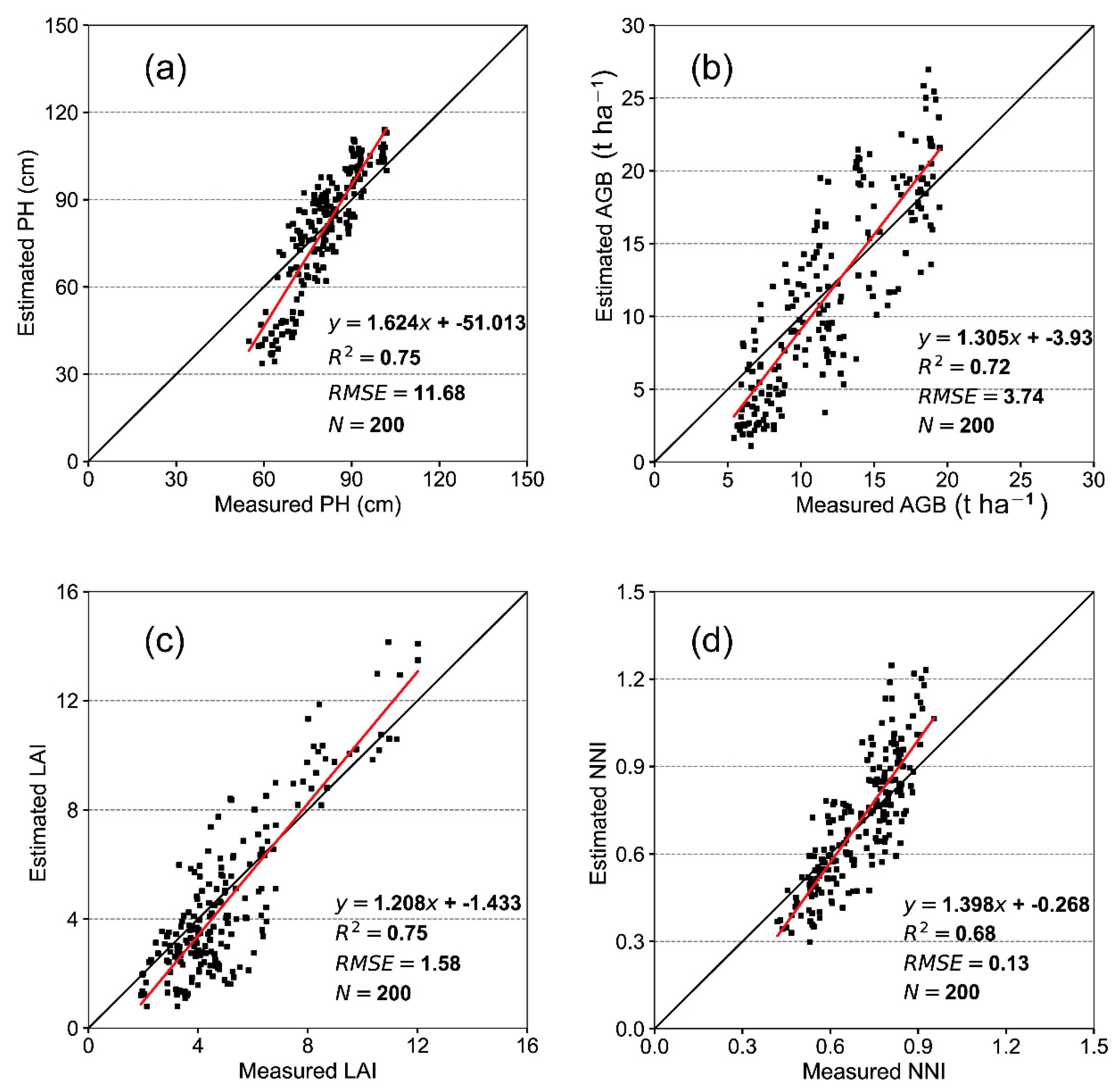
3.5. Test of the RF Model Using V Images

The V images from UAS acquired in 2020 were used to build models which were tested using VI from V images from 2019. Figure 7 shows the scatter plot of the measured variables in 2019. The PH, LAI, AGB, and NNI values estimated by the V image–RF model showed good validation accuracy. The validation accuracies of PH and LAI were the highest, with R2 values of 0.75 and 0.75 and RMSE of 11.68 and 1.58, respectively. The R2 between the measured and estimated AGB was 0.72 and the RMSE was 3.74. For the estimation of NNI, although R2 was slightly smaller, it was still close to 0.7. Therefore, the model established using V images by UAS and the RF algorithm showed promise for monitoring rice growth.

4. Discussion

4.1. Changes of Rice Growth Variables under Different Nitrogen Treatments

By analyzing the measured rice growth variables under different fertilizer treatments in the two experimental fields, in all plots except the unfertilized plots, AGB gradually increased between the jointing and maturity stages, peaking in the maturity stage; NNI gradually decreased, reaching its lowest in the maturity stage; and PH and LAI first increased and then decreased. In the unfertilized plots, AGB gradually increased with the growth stage, but PH, LAI, and NNI did not change significantly in the middle and late growth periods. Rice growth variables did not improve with increasing percentage of controlled-release N fertilizer. However, most growth variables with controlled-release N fertilizer were slightly larger than those with conventional fertilizer and significantly larger than those with reduced N fertilizer and no fertilizer, indicating that the different applications had a relatively large effect on rice growth [57,58]. The key rice growth variables were monitored using V-images and V-NIR images, and the different nitrogen application treatments increased the variability of rice growth between plots, which met the needs of this study.

4.2. Comparison of the V Images and V-NIR Images from UAS

Vegetation canopy structural characteristics and growing conditions are the main factors that affect vegetation canopy reflectance [59]. With the rapid development and popularity of UAS technology, UAS is increasingly being used for crop phenotype monitoring. UAS can carry different types of sensors, each with advantages and disadvantages. Hyperspectral cameras can acquire images with multiple and narrow band information [60]; however, too much spectral information can result in the redundancy of band information [61]. In addition, although studies have shown that crop growth condition monitoring and yield estimation can be achieved using UAS for V-NIR images [62,63], UAS for V-NIR images incurs higher costs than UAS for V images in the application of field crops. Light detection and ranging (LiDAR) technology has also been used to estimate crop height and AGB [64,65]; however, this technology is often unable to accurately estimate relatively short crop canopies. In addition, like hyperspectral cameras, the high cost of LiDAR limits its application in agriculture.
In this study, rice growth variables were monitored using V images and V-NIR images from UAS. Many VIs were extracted using the waveband combinations of these two types of images, all of which correlated well with rice growth variables during certain growth periods. The RF estimation models based on both VI from V-NIR images and V images showed similar results for the tested rice variables. Considering that V images from UAS is much cheaper than V-NIR images from UAS, V images from UAS is more promising for rice variable estimation. However, V-NIR images have rich waveband information which can be useful for particular crop types and monitoring indicators. Therefore, the adaptability of both UAS to different crop types and indicators must be evaluated in future studies.

4.3. Application of RF Algorithm Modeling

The application of linear models for estimating rice growth variables requires each VI to be modeled separately with different variables and the optimal model to be selected manually, which was complex. In addition, only one VI is selected in the modeling process, which makes the models unstable. In recent years, models that combine multiple VIs using machine learning algorithms to estimate crop growth variables have been developed [51,63,66,67]. This study used the RF algorithm, which was determined to be the optimal algorithm by many studies that compared different models for crop monitoring [55,56,68].

4.4. Feasibility of Estimating Rice Growth Variables Using RGB UAS

This study conducted experiments with different rice varieties and fertilization treatments and developed an RF estimation model using V images and V-NIR image by UAS from 2020 combined with the measured growth variables of rice at the jointing, flowering, filling, and maturity periods. The R2 values of PH, LAI, and AGB were all greater than 0.7, and that of NNI was 0.68, which indicated that it was feasible to estimate rice growth variables using V images from UAS and that the RF model established using the V images was suitable for rice growth variable estimation.

5. Conclusions

Under different nitrogen application treatments, pH, AGB, LAI, and NNI significantly differed by growing period. Nitrogen fertilizer significantly impacted rice growth, which provided variability for the estimation of rice growth variables by establishing the correlation between rice growth variables and VIs from images by UAS. When using a simple linear model, the estimations using V-NIR images by UAS were better than those using V images for PH and LAI but worse for AGB and NNI. The RF model improved the estimation accuracy with an R2 greater than 0.8 for every growth period (and greater than 0.9 for the full-growth period). A model test using measured rice variables in a separate year confirmed the effective performance of the RF model established using VI from V Images by UAS. Overall, the V image by UAS was ideal for estimating rice growth variables and was the optimal choice in terms of cost and accuracy.

Author Contributions

Conceptualization, Z.Q. and C.D.; methodology, Z.Q.; software, Z.Q.; validation, F.M., X.X. and Z.L.; formal analysis, Z.Q.; investigation, F.M.; resources, C.D.; data curation, Z.Q.; writing—original draft preparation, Z.Q.; writing—review and editing, Z.Q. and C.D.; visualization, Z.Q. and C.D.; supervision, C.D.; project administration, C.D.; funding acquisition, C.D. All authors have read and agreed to the published version of the manuscript.

Funding

This study was supported by the Key R&D Plan of Shandong Province (2019JZZY010713) and National Key Research and Development Program of China (2018YFE0107000).

Institutional Review Board Statement

Not applicable.

Informed Consent Statement

Not applicable.

Data Availability Statement

Data sharing not applicable.

Conflicts of Interest

The authors declare no conflict of interest.

References

  1. Li, P.; Zhang, X.; Wang, W.; Zheng, H.; Yao, X.; Tian, Y.; Zhu, Y.; Cao, W.; Chen, Q.; Cheng, T. Estimating aboveground and organ biomass of plant canopies across the entire season of rice growth with terrestrial laser scanning. Int. J. Appl. Earth Obs. Geoinf. 2020, 91, 102132. [Google Scholar] [CrossRef]
  2. Fabbri, C.; Mancini, M.; dalla Marta, A.; Orlandini, S.; Napoli, M. Integrating satellite data with a nitrogen nutrition curve for precision top-dress fertilization of durum wheat. Eur. J. Agron. 2020, 120, 126148. [Google Scholar] [CrossRef]
  3. Wang, W.; Yao, X.; Yao, X.; Tian, Y.; Liu, X.; Ni, J.; Cao, W.; Zhu, Y. Estimating leaf nitrogen concentration with three-band vegetation indices in rice and wheat. Field Crops Res. 2012, 129, 90–98. [Google Scholar] [CrossRef]
  4. Fitzgerald, G.; Rodriguez, D.; O’Leary, G. Measuring and predicting canopy nitrogen nutrition in wheat using a spectral index—The canopy chlorophyll content index (CCCI). Field Crops Res. 2010, 116, 318–324. [Google Scholar] [CrossRef]
  5. Bendig, J.; Yu, K.; Aasen, H.; Bolten, A.; Bennertz, S.; Broscheit, J.; Gnyp, M.L.; Bareth, G. Combining UAV-based plant height from crop surface models, visible, and near infrared vegetation indices for biomass monitoring in barley. Int. J. Appl. Earth Obs. Geoinf. 2015, 39, 79–87. [Google Scholar] [CrossRef]
  6. Chakwizira, E.; de Ruiter, J.M.; Maley, S.; Teixeira, E. Evaluating the critical nitrogen dilution curve for storage root crops. Field Crops Res. 2016, 199, 21–30. [Google Scholar] [CrossRef]
  7. Giletto, C.M.; Echeverría, H.E. Critical nitrogen dilution curve for processing potato in argentinean humid pampas. Am. J. Potato Res. 2011, 89, 102–110. [Google Scholar] [CrossRef]
  8. Raj, R.; Walker, J.P.; Pingale, R.; Nandan, R.; Naik, B.; Jagarlapudi, A. Leaf area index estimation using top-of-canopy airborne RGB images. Int. J. Appl. Earth Obs. Geoinf. 2021, 96, 102282. [Google Scholar] [CrossRef]
  9. Behera, S.K.; Srivastava, P.; Pathre, U.V.; Tuli, R. An indirect method of estimating leaf area index in Jatropha curcas L. using LAI-2000 Plant Canopy Analyzer. Agric. For. Meteorol. 2010, 150, 307–311. [Google Scholar] [CrossRef]
  10. Nguy-Robertson, A.; Peng, Y.; Arkebauer, T.; Scoby, D.; Schepers, J.; Gitelson, A. Using a simple leaf color chart to estimate leaf and canopy chlorophyll content in maize (Zea mays). Commun. Soil Sci. Plant. Anal. 2015, 46, 2734–2745. [Google Scholar] [CrossRef]
  11. Wang, Y.; Shi, P.; Zhang, G.; Ran, J.; Shi, W.; Wang, D. A critical nitrogen dilution curve for japonica rice based on canopy images. Field Crops Res. 2016, 198, 93–100. [Google Scholar] [CrossRef]
  12. Tsui, O.W.; Coops, N.C.; Wulder, M.A.; Marshall, P.L.; McCardle, A. Using multi-frequency radar and discrete-return LiDAR measurements to estimate above-ground biomass and biomass components in a coastal temperate forest. ISPRS J. Photogramm. Remote Sens. 2012, 69, 121–133. [Google Scholar] [CrossRef]
  13. Zhu, X.; Liu, D. Improving forest aboveground biomass estimation using seasonal Landsat NDVI time-series. ISPRS-J. Photogramm. Remote Sens. 2015, 102, 222–231. [Google Scholar] [CrossRef]
  14. Verger, A.; Filella, I.; Baret, F.; Penuelas, J. Vegetation baseline phenology from kilometric global LAI satellite products. Remote Sens. Environ. 2016, 178, 1–14. [Google Scholar] [CrossRef] [Green Version]
  15. Kross, A.; McNairn, H.; Lapen, D.; Sunohara, M.; Champagne, C. Assessment of RapidEye vegetation indices for estimation of leaf area index and biomass in corn and soybean crops. Int. J. Appl. Earth Obs. Geoinf. 2015, 34, 235–248. [Google Scholar] [CrossRef] [Green Version]
  16. Wu, S.; Yang, P.; Ren, J.; Chen, Z.; Liu, C.; Li, H. Winter wheat LAI inversion considering morphological characteristics at different growth stages coupled with microwave scattering model and canopy simulation model. Remote Sens. Environ. 2020, 240, 111681. [Google Scholar] [CrossRef]
  17. Croft, H.; Arabian, J.; Chen, J.M.; Shang, J.; Liu, J. Mapping within-field leaf chlorophyll content in agricultural crops for nitrogen management using Landsat-8 imagery. Precis. Agric. 2019, 21, 856–880. [Google Scholar] [CrossRef] [Green Version]
  18. Wiseman, G.; McNairn, H.; Homayouni, S.; Shang, J. RADARSAT-2 polarimetric SAR response to crop biomass for agricultural production monitoring. IEEE J. Sel. Top. Appl. Earth Observ. Remote Sens. 2014, 7, 4461–4471. [Google Scholar] [CrossRef]
  19. Weiss, M.; Jacob, F.; Duveiller, G. Remote sensing for agricultural applications: A meta-review. Remote Sens. Environ. 2020, 236, 111402. [Google Scholar] [CrossRef]
  20. Duan, T.; Chapman, S.C.; Guo, Y.; Zhen, B. Dynamic monitoring of NDVI in wheat agronomy and breeding trials using an unmanned aerial vehicle. Field Crops Res. 2017, 210, 71–80. [Google Scholar] [CrossRef]
  21. Jin, X.; Zarco-Tejada, P.; Schmidhalter, U.; Reynolds, M.P.; Hawkesford, M.J.; Varshney, R.K.; Yang, T.; Nie, C.; Li, Z.; Ming, B.; et al. High-throughput estimation of crop traits: A review of ground and aerial phenotyping platforms. IEEE Geosci. Remote Sens. Mag. 2021, 9, 200–231. [Google Scholar] [CrossRef]
  22. Verger, A.; Vigneau, N.; Chéron, C.; Gilliot, J.M.; Comar, A.; Baret, F. Green area index from an unmanned aerial system over wheat and rapeseed crops. Remote Sens. Environ. 2014, 152, 654–664. [Google Scholar] [CrossRef]
  23. Maimaitijiang, M.; Ghulam, A.; Sidike, P.; Hartling, S.; Maimaitiyiming, M.; Peterson, K.; Shavers, E.; Fishman, J.; Peterson, J.; Kadam, S.; et al. Unmanned aerial system (UAS)-based phenotyping of soybean using multi-sensor data fusion and extreme learning machine. ISPRS-J. Photogramm. Remote Sens. 2017, 134, 43–58. [Google Scholar] [CrossRef]
  24. Jin, X.; Liu, S.; Baret, F.; Hemerlé, M.; Comar, A. Estimates of plant density of wheat crops at emergence from very low altitude UAV imagery. Remote Sens. Environ. 2017, 198, 105–114. [Google Scholar] [CrossRef] [Green Version]
  25. Brook, A.; De Micco, V.; Battipaglia, G.; Erbaggio, A.; Ludeno, G.; Catapano, I.; Bonfante, A. A smart multiple spatial and temporal resolution system to support precision agriculture from satellite images: Proof of concept on aglianico vineyard. Remote Sens. Environ. 2020, 240, 111679. [Google Scholar] [CrossRef]
  26. Lu, J.; Li, W.; Yu, M.; Zhang, X.; Ma, Y.; Su, X.; Yao, X.; Cheng, T.; Zhu, Y.; Cao, W.; et al. Estimation of rice plant potassium accumulation based on non-negative matrix factorization using hyperspectral reflectance. Precis. Agric. 2020, 22, 51–74. [Google Scholar] [CrossRef]
  27. Bian, J.; Zhang, Z.; Chen, J.; Chen, H.; Cui, C.; Li, X.; Chen, S.; Fu, Q. Simplified evaluation of cotton water stress using high resolution unmanned aerial vehicle thermal imagery. Remote Sens. 2019, 11, 267. [Google Scholar] [CrossRef] [Green Version]
  28. Yue, J.; Yang, G.; Tian, Q.; Feng, H.; Xu, K.; Zhou, C. Estimate of winter-wheat above-ground biomass based on UAV ultrahigh-ground-resolution image textures and vegetation indices. ISPRS-J. Photogramm. Remote Sens. 2019, 150, 226–244. [Google Scholar]
  29. Tao, H.; Feng, H.; Xu, L.; Miao, M.; Long, H.; Yue, J.; Li, Z.; Yang, G.; Yang, X.; Fan, L. Estimation of crop growth parameters using UAV-based hyperspectral remote sensing data. Sensors 2020, 20, 1296. [Google Scholar] [CrossRef] [PubMed] [Green Version]
  30. Tao, H.; Feng, H.; Xu, L.; Miao, M.; Yang, G.; Yang, X.; Fan, L. Estimation of the yield and plant height of winter wheat using UAV-based hyperspectral images. Sensors 2020, 20, 1231. [Google Scholar] [CrossRef] [PubMed] [Green Version]
  31. Zhang, X.; Zhao, J.; Yang, G.; Liu, J.; Cao, J.; Li, C.; Zhao, X.; Gai, J. Establishment of plot-yield prediction models in soybean breeding programs using UAV-based hyperspectral remote sensing. Remote Sens. 2019, 11, 2752. [Google Scholar] [CrossRef] [Green Version]
  32. Zheng, H.; Cheng, T.; Zhou, M.; Li, D.; Yao, X.; Tian, Y.; Cao, W.; Zhu, Y. Improved estimation of rice aboveground biomass combining textural and spectral analysis of UAV imagery. Precis. Agric. 2018, 20, 611–629. [Google Scholar] [CrossRef]
  33. Li, B.; Xu, X.; Zhang, L.; Han, J.; Bian, C.; Li, G.; Liu, J.; Jin, L. Above-ground biomass estimation and yield prediction in potato by using UAV-based RGB and hyperspectral imaging. ISPRS J. Photogramm. Remote Sens. 2020, 162, 161–172. [Google Scholar] [CrossRef]
  34. Mutanga, O.; Skidmore, A.K. Narrow band vegetation indices overcome the saturation problem in biomass estimation. Int. J. Remote Sens. 2010, 25, 3999–4014. [Google Scholar] [CrossRef]
  35. Singh, A.; Ganapathysubramanian, B.; Singh, A.K.; Sarkar, S. Machine learning for high-throughput stress phenotyping in plants. Trends Plant. Sci. 2016, 21, 110–124. [Google Scholar] [CrossRef] [PubMed] [Green Version]
  36. Gahrouei, O.R.; McNairn, H.; Hosseini, M.; Homayouni, S. Estimation of crop biomass and leaf area index from multitemporal and multispectral imagery using machine learning approaches. Can. J. Remote Sens. 2020, 46, 84–99. [Google Scholar] [CrossRef]
  37. Wang, L.; Zhou, X.; Zhu, X.; Dong, Z.; Guo, W. Estimation of biomass in wheat using random forest regression algorithm and remote sensing data. Crop J. 2016, 4, 212–219. [Google Scholar] [CrossRef] [Green Version]
  38. Louhaichi, M.; Borman, M.M.; Johnson, D.E. Spatially located platform and aerial photography for documentation of grazing impacts on wheat. Geocarto Int. 2008, 16, 65–70. [Google Scholar] [CrossRef]
  39. Tucker, C.J. Red and photographic infrared linear combinations for monitoring vegetation. Remote Sens. Environ. 1979, 8, 127–150. [Google Scholar] [CrossRef] [Green Version]
  40. Yang, B.; Wang, M.; Sha, Z.; Wang, B.; Chen, J.; Yao, X.; Cheng, T.; Cao, W.; Zhu, Y. Evaluation of aboveground nitrogen content of winter wheat using digital imagery of unmanned aerial vehicles. Sensors 2019, 19, 4416. [Google Scholar] [CrossRef] [Green Version]
  41. Meyer, G.E.; Neto, J.C. Verification of color vegetation indices for automated crop imaging applications. Comput. Electron. Agric. 2008, 63, 282–293. [Google Scholar] [CrossRef]
  42. Qi, J.; Chehbouni, A.; Huete, A.R.; Kerr, Y.H.; Sorooshian, S. A modified soil adjusted vegetation index. Remote Sens. Environ. 1994, 48, 119–126. [Google Scholar] [CrossRef]
  43. Woebbecke, D.M.; Meyer, G.E.; Bargen, K.V.; Mortensen, D.A. Color indices for weed identification under various soil, residue, and lighting conditions. Trans. ASAE 1995, 38, 259–269. [Google Scholar] [CrossRef]
  44. Saberioon, M.M.; Gholizadeh, A. Novel approach for estimating nitrogen content in paddy fields using low altitude remote sensing system. ISPRS Int. Arch. Photogramm. Remote Sens. Spat. Info. Sci. 2016, 41, 1011–1015. [Google Scholar] [CrossRef] [Green Version]
  45. Possoch, M.; Bieker, S.; Hoffmeister, D.; Bolten, A.; Schellberg, J.; Bareth, G. Multi-temporal crop surface models combined with the rgb vegetation index from uav-based images for forage monitoring in grassland. ISPRS Int. Arch. Photogramm. Remote Sens.Spa. Info. Sci. 2016, 41, 991–998. [Google Scholar]
  46. Verrelst, J.; Schaepman, M.E.; Koetz, B.; Kneubühler, M. Angular sensitivity analysis of vegetation indices derived from CHRIS/PROBA data. Remote Sens. Environ. 2008, 112, 2341–2353. [Google Scholar] [CrossRef]
  47. Zheng, H.; Cheng, T.; Li, D.; Yao, X.; Tian, Y.; Cao, W.; Zhu, Y. Combining unmanned aerial vehicle (UAV)-based multispectral imagery and ground-based hyperspectral data for plant nitrogen concentration estimation in rice. Front. Plant. Sci. 2018, 9, 936. [Google Scholar] [CrossRef] [PubMed]
  48. Fitzgerald, G.J.; Rodriguez, D.; Christensen, L.K.; Belford, R.; Sadras, V.O.; Clarke, T.R. Spectral and thermal sensing for nitrogen and water status in rainfed and irrigated wheat environments. Precis. Agric. 2006, 7, 233–248. [Google Scholar] [CrossRef]
  49. Fu, Z.; Jiang, J.; Gao, Y.; Krienke, B.; Wang, M.; Zhong, K.; Cao, Q.; Tian, Y.; Zhu, Y.; Cao, W.; et al. Wheat growth monitoring and yield estimation based on multi-rotor unmanned aerial vehicle. Remote Sens. 2020, 12, 508. [Google Scholar] [CrossRef] [Green Version]
  50. Li, S.; Ding, X.; Kuang, Q.; Ata-Ui-Karim, S.T.; Cheng, T.; Liu, X.; Tian, Y.; Zhu, Y.; Cao, W.; Cao, Q. Potential of UAV-based active sensing for monitoring rice leaf nitrogen status. Front. Plant. Sci. 2018, 9, 1834. [Google Scholar] [CrossRef] [Green Version]
  51. Han, L.; Yang, G.; Dai, H.; Xu, B.; Yang, H.; Feng, H.; Li, Z.; Yang, X. Modeling maize above-ground biomass based on machine learning approaches using UAV remote-sensing data. Plant. Methods 2019, 15, 10. [Google Scholar] [CrossRef] [PubMed] [Green Version]
  52. Steven, M.D. The sensitivity of the OSAVI vegetation index to observational parameters. Remote Sens. Environ. 1998, 63, 49–60. [Google Scholar] [CrossRef]
  53. Yue, J.; Yang, G.; Li, C.; Li, Z.; Wang, Y.; Feng, H.; Xu, B. Estimation of winter wheat above-ground biomass using unmanned aerial vehicle-based snapshot hyperspectral sensor and crop height improved models. Remote Sens. 2017, 9, 708. [Google Scholar] [CrossRef] [Green Version]
  54. Haboudane, D. Hyperspectral vegetation indices and novel algorithms for predicting green LAI of crop canopies: Modeling and validation in the context of precision agriculture. Remote Sens. Environ. 2004, 90, 337–352. [Google Scholar] [CrossRef]
  55. Zha, H.; Miao, Y.; Wang, T.; Li, Y.; Zhang, J.; Sun, W.; Feng, Z.; Kusnierek, K. Improving unmanned aerial vehicle remote sensing-based rice nitrogen nutrition index prediction with machine learning. Remote Sens. 2020, 12, 215. [Google Scholar] [CrossRef] [Green Version]
  56. Osco, L.P.; Ramos, A.M.P.; Pereira, D.R.; Moriy, E.A.S.; Imai, N.N.; Matsubara, E.T.; Estrabis, N.; de Souza, M.; Marcato, J.; Gonçalves, W.N.; et al. Predicting canopy nitrogen content in citrus-trees using random forest algorithm associated to spectral vegetation indices from UAV-imagery. Remote Sens. 2019, 11, 2925. [Google Scholar] [CrossRef] [Green Version]
  57. Chen, B.; Yang, H.; Song, W.; Liu, C.; Xu, J.; Zhao, W.; Zhou, Z. Effect of N fertilization rate on soil alkali-hydrolyzable N, subtending leaf N concentration, fiber yield, and quality of cotton. Crop J. 2016, 4, 323–330. [Google Scholar] [CrossRef] [Green Version]
  58. Watts, D.B.; Runion, G.B.; Balkcom, K.S. Nitrogen fertilizer sources and tillage effects on cotton growth, yield, and fiber quality in a coastal plain soil. Field Crops Res. 2017, 201, 184–191. [Google Scholar] [CrossRef]
  59. Sahadevan, A.S.; Shrivastava, P.; Das, B.S.; Sarathjith, M.C. Discrete wavelet transform approach for the estimation of crop residue mass from spectral reflectance. IEEE J. Sel. Top. Appl. Earth Observ. Remote Sens. 2014, 7, 2490–2495. [Google Scholar] [CrossRef]
  60. Ge, X.; Ding, J.; Jin, X.; Wang, J.; Chen, X.; Li, X.; Liu, J.; Xie, B. Estimating agricultural soil moisture content through UAV-based hyperspectral images in the arid region. Remote Sens. 2021, 13, 1562. [Google Scholar] [CrossRef]
  61. Shi, T.; Wang, J.; Chen, Y.; Wu, G. Improving the prediction of arsenic contents in agricultural soils by combining the reflectance spectroscopy of soils and rice plants. IEEE J. Sel. Top. Appl. Earth Observ. Remote Sens. 2016, 52, 95–103. [Google Scholar] [CrossRef]
  62. Chen, Z.; Miao, Y.; Lu, J.; Zhou, L.; Li, Y.; Zhang, H.; Lou, W.; Zhang, Z.; Kusnierek, K.; Liu, C. In-season diagnosis of winter wheat nitrogen status in smallholder farmer fields across a village using unmanned aerial vehicle-based remote sensing. Agronomy 2019, 9, 619. [Google Scholar] [CrossRef] [Green Version]
  63. Li, F.; Piasecki, C.; Millwood, R.J.; Wolfe, B.; Mazarei, M.; Stewart, C.N.; Steward, C.N. High-throughput switchgrass phenotyping and biomass modeling by UAV. Front. Plant. Sci. 2020, 11, 574073. [Google Scholar] [CrossRef]
  64. Li, W.; Niu, Z.; Wang, C.; Huang, W.; Chen, H.; Gao, S.; Li, D.; Muhammad, S. Combined use of airborne LiDAR and Satellite GF-1 data to estimate leaf area index, height, and aboveground biomass of maize during peak growing season. IEEE J. Sel. Top. Appl. Earth Observ. Remote Sens. 2015, 8, 4489–4501. [Google Scholar] [CrossRef]
  65. Qiu, Z.; Xiang, H.; Ma, F.; Du, C. Qualifications of rice growth indicators optimized at different growth stages using unmanned aerial vehicle digital imagery. Remote Sens. 2020, 12, 3228. [Google Scholar] [CrossRef]
  66. Wang, Y.; Zhang, K.; Tang, C.; Cao, Q.; Tian, Y.; Zhu, Y.; Cao, W.; Liu, X. Estimation of rice growth parameters based on linear mixed-effect model using multispectral images from fixed-wing unmanned aerial vehicles. Remote Sens. 2019, 11, 1371. [Google Scholar] [CrossRef] [Green Version]
  67. Shi, P.; Wang, Y.; Xu, J.; Zhao, Y.; Yang, B.; Yuan, Z.; Sun, Q. Rice nitrogen nutrition estimation with RGB images and machine learning methods. Comput. Electron. Agric. 2021, 180, 105860. [Google Scholar] [CrossRef]
  68. Osco, L.P.; Ramos, A.P.M.; Pinheiro, M.M.F.; Moriya, E.A.S.; Imai, N.N.; Estrabis, N.; Ianczyk, F.; de Araujo, F.F.; Liesenberg, V.; Jorge, L.; et al. A machine learning framework to predict nutrient content in valencia-orange leaf hyperspectral measurements. Remote Sens. 2020, 12, 906. [Google Scholar] [CrossRef] [Green Version]
Figure 1. Location and images of the experimental plots with different nitrogen treatments. (a) location of Pukou and Luhe in Nanjing City, Jiangsu Province, China; (b) image of Pukou experimental plots with five fertilization treatments and regions for sampling and VI extraction; N1, N2, N3, N4, and N5 represented different N fertilization treatments; (c) image of Luhe experimental plots with three fertilization treatments and regions for sampling and VI extraction; Na, Nb, and Nc represented different N fertilization treatments).
Remotesensing 14 01384 g001
Figure 2. (a) UAS with digital camera for V images, (b) UAS with multispectral camera for V-NIR images, and (c) diffuse reflective plates.
Remotesensing 14 01384 g002
Figure 3. Diagram of the method overview in this study. (PH, rice plant height; LAI, leaf area index; AGB, aboveground biomass; NNI, nitrogen nutrient index; VIs, vegetation indices; V, visible; NIR, near infrared; RF, random forest.
Remotesensing 14 01384 g003
Figure 4. Histograms of rice growth variables under different nitrogen treatments at different periods: (a,e) PH, (b,f), AGB, (c,g) LAI, and (d,h) NNI in the Pukou and Luhe experiments, respectively. N5, N4, N3, N2, N1 were different nitrogen treatments in Pukou experiment and Na, Nb, Nc were different nitrogen treatments in Luhe experiment.
Remotesensing 14 01384 g004
Figure 5. Comparison of validation results of RF models used for estimating (a) PH, (b) AGB, (c) LAI, and (d) NNI using V images and V-NIR images at different growth periods.
Remotesensing 14 01384 g005
Figure 6. Validations of (a,b) pH, (c,d) LAI, (e,f) AGB, and (g,h) NNI with RF models based on VI from V images and V-NIR images, respectively, in full growth stage.
Remotesensing 14 01384 g006
Figure 7. Test plots of measured and estimated values using the established V image–RF model in the full growth stage in 2020. Tests of (a) PH; (b) LAI; (c) AGB; and (d) NNI in 2019.
Remotesensing 14 01384 g007
Table 1. Fertilization treatments in field experiments.
Experimental SiteNitrogen TreatmentsTotal Nitrogen Rate (kg)Proportion of Controlled-Release Nitrogen
PukouN100
N2240 kg ha−10
N3240 kg ha−130%
N4240 kg ha−140%
N5240 kg ha−150%
LuheNa196 kg ha−10
Nb196 kg ha−140%
Nc196 kg ha−150%
Table 2. Descriptive statistics of PH, AGB, LAI, and NNI at different stages of rice.
DateGrowth VariablesMeanMedianStandard DeviationMinMaxN
JointingPH (cm)63.0760.0018.0433.6795.00100
AGB (t ha−1)4.503.402.941.1113.58100
LAI4.773.812.741.8514.15100
NNI0.910.950.210.371.29100
FloweringPH (cm)88.3489.0011.7063.33110.0100
AGB (t ha−1)8.647.733.893.1520.50100
LAI4.183.792.041.1110.76100
NNI0.720.740.190.341.09100
FillingPH (cm)89.1190.8313.9455.67122.0100
AGB (t ha−1)11.9711.064.183.4021.46100
LAI4.444.002.530.8014.09100
NNI0.580.560.190.251.05100
MaturityPH (cm)92.7793.0010.3672.00116.0100
AGB (t ha−1)16.1015.914.407.0526.96100
LAI2.982.711.400.798.35100
NNI0.510.470.130.260.81100
Table 3. List of VIs from V images and V-NIR images used in this study.
Indices OriginVegetation IndicesFormulationReferences
Vegetation indices from visible imagesGreen Leaf algorithm (GLA)(2 × g − r − b)/(2 × g + r + b)[38]
Green Leaf Index (GLI)(2 × g − r + b)/(2 × g + r + b)[38]
Green Red Vegetation Index (GRVI)(g − r)/(g + r)[39]
Modified Green Red Vegetation Index (MGRVI)(g2 − r2)/(g2 + r2)[5]
Excess Green minus Excess Red (ExGR)(2 × g − r − b) − (1.4 × r − g)[40]
Excess Red Vegetation Index (ExR)(1.4 × r) − g[41]
Excess Blue Vegetation Index (ExB)(1.4 × b) − g[42]
Excess Green Vegetation Index (ExG)(2 × g) − r − b[43]
Visible Atmospherically Resistant Index (VARI)(g − r)/(g + r − b)[44]
Red Green Blue Vegetation Index (RGBVI)(g2 − b × r2)/(g2 + b × r2)[45]
Red Green Ratio Index (RGRI)r/g[46]
Vegetation
Indices from V-NIR images
Normalized different vegetation index (NDVI)(NIR − R)/(NIR + R)[47,48]
Normalized difference red-edge (NDRE)(NIR − RE)/(NIR + RE)[48]
Soil-adjusted vegetation index (SAVI)(1 + L) × (NIR − R)/(NIR + RE + L); L = 0.5[49]
Red edge ration vegetation index (RERVI)NIR/RE[50]
Red edge difference vegetation index (REDVI)NIR − RE[50]
Ration vegetation index (RVI)R/NIR[50,51]
Optimized soil-adjusted vegetation index (OSAVI)(NIR − R)/(NIR + R + 0.16)[52]
Renormalized difference vegetation index (RDVI)(NIR − R)/SQRT(NIR + R)[53,54]
Enhanced vegetation index (EVI)2.4 × (NIR − RE)/(NIR + RE + 1)[53]
Note: r, g, and b represent the reflectance values of the red, green, and blue bands of the V images, respectively; and R, NIR, and RE represent the reflectance values of the red, near-infrared, and red-edge bands of the V-NIR images, respectively.
Table 4. Correlation coefficients of rice growth variables with VIs from V images and V-NIR images in different growth periods.
Physiological
Variables
Growth StagesVI from V ImagesVI from V-NIR Images
Optimal VIR2Optimal VIR2
PHJointingVARI0.52 ***REDVI0.57 ***
FloweringRGRI0.15RERVI0.34 **
FillingMGRVI0.50 ***NDRE0.53 ***
MaturityRGBVI0.14RVI0.30 **
AGBJointingVARI0.62 ***SAVI0.58 ***
FloweringExB0.20RERVI0.16
FillingExB0.35 **NDRE0.26 *
MaturityGLI0.39 **RVI0.29 *
LAIJointingVARI0.60 ***EVI0.62 ***
FloweringRGRI0.19RERVI0.41 ***
FillingRGBVI0.48 **NDRE0.57 ***
MaturityGLA0.56 ***RVI0.57 ***
NNIJointingExGR0.47 ***NDVI0.42 ***
FloweringMGRVI0.33 **REDVI0.28 *
FillingGRVI0.48 ***NDRE0.35 **
MaturityVARI0.79 ***REDVI0.76 ***
* 10% level of significance with p-values between 0.05 and 0.1; ** 5% level of significance with p-values between 0.01 and 0.05; *** 1% level of significance with p-values less than 0.01; 50 samples from 2020 were involved in each linear correlation analysis. VARI, visible atmospherically resistant index; RGRI, red-green ratio index; MGRVI, modified green red vegetation index; RGBVI, red green blue vegetation index; VARI, visible atmospherically resistant index; ExB, Excess blue vegetation index; GLI, green leaf index; GLA, green Leaf algorithm; ExGR, excess green minus excess red; GRVI, green red vegetation index; REDVI, red edge difference vegetation index; RERVI, red edge ration vegetation index; NDRE, normalized difference red-edge; RVI, ration vegetation index; SAVI, soil-adjusted vegetation index; EVI, enhanced vegetation index; NDVI, normalized difference vegetation index.
Publisher’s Note: MDPI stays neutral with regard to jurisdictional claims in published maps and institutional affiliations.

