Framework for Remote Sensing and Modelling of Lithium-Brine Deposit Formation

Abstract

The demand for “green” metals such as lithium is increasing as the world works to reduce its reliance on fossil fuels. More than half of the world’s lithium resources are contained in lithium-brine deposits, including the salt flats, or “salars”, of the Andean region of South America, also known as the Lithium Triangle. The genesis of lithium-brine deposits is largely driven by the leaching of lithium from source rocks in watersheds, transport via groundwater systems to salars, and evaporative concentration in salars. The goal of this research is to create a consistent and seamless methodology for tracking lithium mass from its source in the watershed to its greatest concentration in the nucleus. The area of interest is in and around Bolivia’s Salar de Uyuni, the world’s largest salt flat. We explore how Li-brine deposits form, where the water and solute come from, how the brines are formed, and how abstraction affects the mass balance inside the salar. To support the entire system, open-source Earth observation (EO) data are analysed. We found that by constructing a flexible and repeatable workflow, the question of how lithium reaches the Salar de Uyuni can be addressed. The work demonstrated the importance of groundwater flow to the river network and highlighted the need for flow data for the main river supplying the salar with both water inflow and lithium mass.

1. Introduction

Net-zero policies necessitate a shift to cleaner transportation and renewable energy storage, but energy and mineral supply chains face numerous challenges. From a mineral standpoint, low-carbon technology is demanding. The World Bank predicts that more than 3 billion tonnes of minerals and metals will be required to deploy solar, wind, and geothermal power, as well as energy storage, if our planet is to stay within the COP21 Paris Agreement target of a global average temperature increase of well below 2 °C. In light of this, demand for battery metals such as cobalt and lithium is expected to rise 500% from current levels by 2050 [1]. The speed and scale with which green energy technologies can reduce greenhouse gas emissions and enable climate-resilient growth will be determined by mineral availability.

Electric vehicles, which use Li-ion rechargeable batteries as a key component, are at the forefront of green technology. Lithium is also used for the production of other batteries, such as cell phones and laptops. The battery market currently takes 71% of global lithium production. Lithium is also employed in the ceramics and glass industries, accounting for 14% of the production [2]. Various other uses, including lubricating greases and air purification, take the remaining 15%. Rapid growth in demand is driven by the battery market, which increased by 48% in 10 years (2010–2020). Worldwide lithium production rose more than 300% from 25,300 tonnes in 2010 to 82,000 tonnes in 2020 [2,3].

Within this context, the search for and extraction of lithium are becoming an important revenue source for many world economies. In particular, the U.S. Geological Survey [2] estimates that the first three producers lie within the South American “Lithium Triangle”, i.e., Bolivia, with 21 million tonnes resources; Argentina, with 19.3 Mt; and Chile, with 9.6 Mt. Other important producers are the United States, with 7.9 Mt, and Australia, with 6.4 Mt. Security of supply of lithium to the global markets and increasing expectations by consumers for responsibly sourced raw materials result in a growing global interest in lithium resources and their extraction.

Lithium is extracted from three types of deposits: “hard-rock” pegmatites, continental brines in “salars”, and hydrothermally altered clays. Brine deposits account for around 75% of the world’s lithium, due to lower costs of extraction [4,5]. Li-rich brines are found predominantly in basins of internal drainage or salars which are mainly located in the Andes in the Lithium Triangle countries. They are endorheic basins, meaning that the only exit for the inflowing water is via evaporation. This means that water, rich in lithium, flows to the salars and is then evaporated, concentrating the minerals. Over long time periods (~Ma), high-density brines collect in a nucleus that contains economic concentrations of lithium which is then pumped out. Whilst extraction from rocks requires a hydrometallurgical process (crushing and heating), extraction from brines, i.e., saline aquifers, involves the pumping from the shallow subsurface and a set of solar evaporation ponds where the liquid solution is moved from one to another until a desired concentration, or “purity”, is reached. In this process, other components are removed by either precipitation or chemical reactions through the introduction of reagents. This is necessary since lithium coexists in brines with other elements, such as magnesium, that are noneconomic. To be noted, the evaporation/precipitation process is a slow one, taking one to two years from the water pumping to the processing of the concentrated brine in the processing plant, where a further processing is employed to produce lithium carbonate [5].

The Salar de Uyuni in Bolivia (Figure 1) is being used as a study area for developing a repeatable and seamless workflow for tracking lithium from its source in the watershed to the salar nucleus at its maximum concentration. It gives a systems-based knowledge of the genesis of lithium-brine deposits, which can help with broader issues such as resource reporting and establishing uncertainty bounds to resource estimations. It is outwith the purpose of the study to develop sociopolitical considerations regarding the extraction, and this work is a purely technological one, making use of a combination of several scientific disciplines, i.e., remote sensing, geology, and hydrology. Nevertheless, given the study area, it is worth summarising the work of Barandiarán, who analysed sociopolitical debates in the Lithium Triangle [6]. Just focusing on Bolivia, which has yet to start large-scale commercialisation, Barandiarán concluded that lithium is used to build a sociotechnical imagery where the government supports scientific and technological research and development, achieved by Bolivian-trained scientists, to embody political values linked to the modernisation of the nation.

Remote sensing is being widely used for geological applications [7]. Some Earth observation missions are specifically built with geology as the principal application area, such as the multispectral Advanced Spaceborne Thermal Emission and Reflection Radiometer (ASTER) [8]. Indeed, geological applications are particularly effective with data capturing short-wave infrared (SWIR) and thermal infrared (TIR) electromagnetic bands, where the largest spectral variations are taking place, thus allowing accurate land cover discrimination. Among geological applications, examples useful to this study are around (1) fault and lineament mapping [9,10], where digital elevation models (DEMs) and multispectral data are used in relation to geomorphological variations and colour/spectral changes; (2) alteration unit mapping [11,12], where multispectral data and techniques such as principal component analysis (PCA) and spectral angle mapping are used to derive iron oxide minerals, hydrothermal alteration zones, and other units; (3) mineral quantification mapping and lithological discrimination [13,14], where multi- and hyperspectral data are used to detect specific mineral spectral features, e.g., absorption bands, for sedimentary, igneous, and metamorphic rocks; and (4) groundwater investigation [15,16], where several types of remote sensing technologies are used to derive indicators of groundwater, since remote sensing cannot penetrate deep into surface. Typical groundwater indicators are features associated with recharge zones (rivers, lakes, etc.), discharge zones (springs, etc.), soil moisture, landforms, drainage characteristics, depth of weathering, and all the indicators derived from the above-described applications [7].

Remote sensing of lithium deposits is a relatively new application and only a few studies have been published, also reviewed by Cardoso et al. [17], with a few papers published by the same research group in scientific journals (e.g., [18]) and a few other conference proceedings. Specifically, refs [17,18,19,20] cover the extraction from rocks and address the detection of Li-bearing pegmatites through spectral analysis. There are several limitations for an accurate discrimination, linked to the degree of weathering of the host rock, the vegetation covering, and the potential need for thermal bands [17]. Rossi et al. [21] instead covers the extraction from subterranean brines with an approach that combines several geological and geobotanical proxies. The study presented in this paper is the first study covering the genesis of lithium brines in salt lakes; it does not focus on the mineral exploration of extraction itself, i.e., the derivation of a prospectivity map, but provides an evidence-based model and more general hydrogeological framework that employs satellite remotely sensed data to describe the source of lithium and its movement in the environment. To be noted, the derivation of hydrogeological frameworks with ground data is a common and old practice, an example being the study in [22], which defined the hydraulic character and subsurface distribution of the major aquifers and aquitards, including their areas of recharge and discharge and the rate and the direction of groundwater movement for a test site in Nevada, United States.

The paper is structured as follows: Section 2 describes the test site and presents the data used in the study alongside its processing. Section 3 presents the geological processing and related workflow, and Section 4 and Section 5 present the hydrogeology and mass balance workflows, respectively. Finally, Section 6 discusses the generic lithium movement framework and traces the investigation conclusions.

2. Materials and Methods

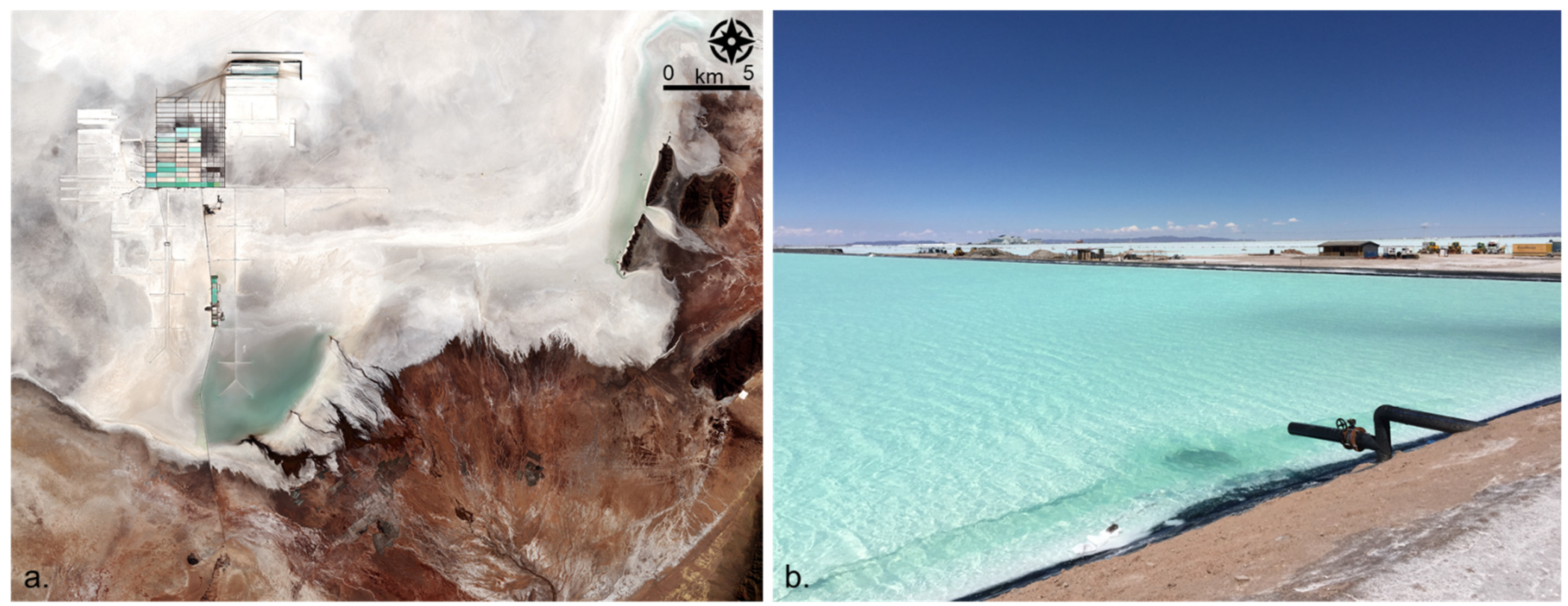
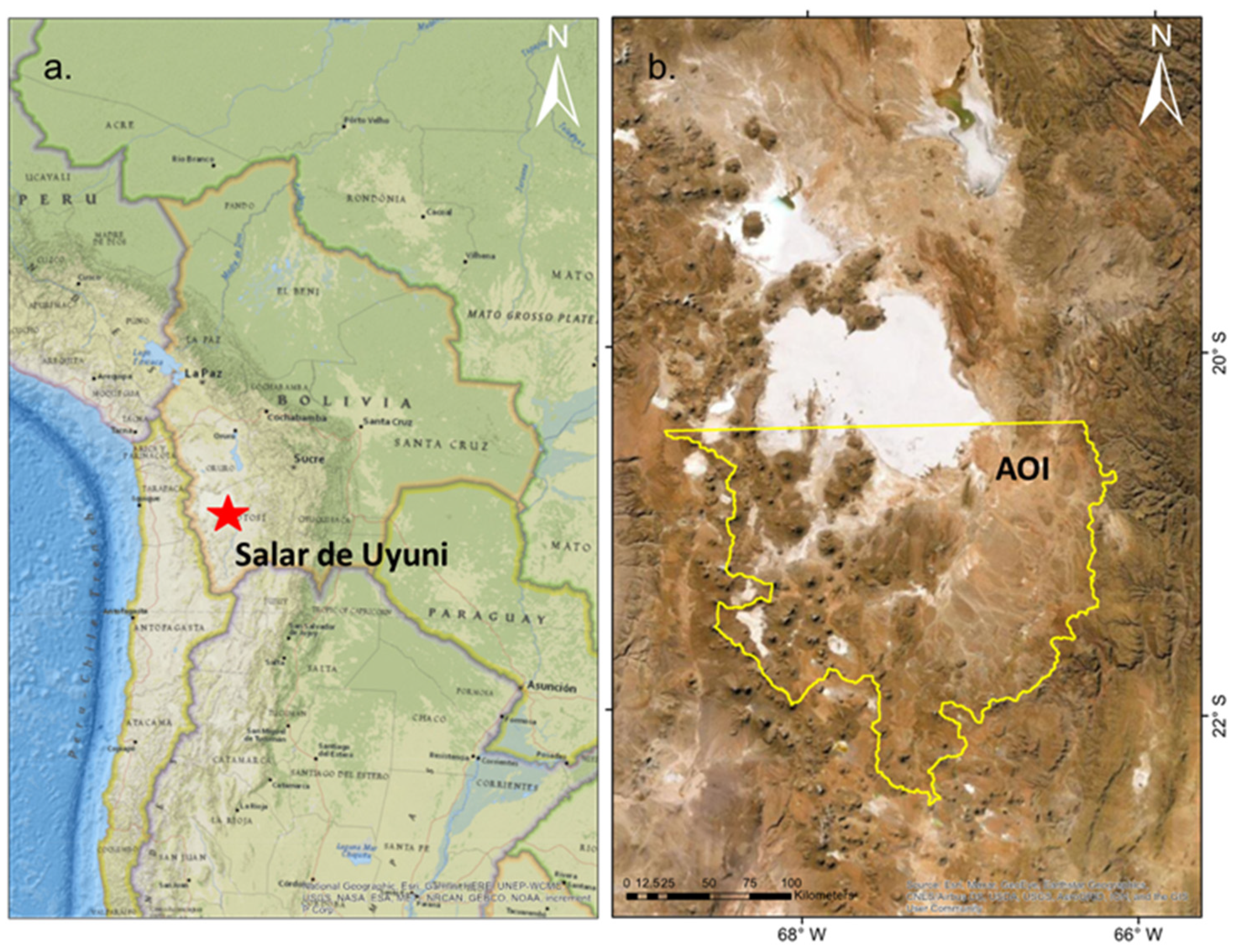
2.1. Test Site

Salars are essentially inland salt flats that form in arid conditions, and notable examples are those that are found in the Lithium Triangle in the central Andes of Bolivia, Chile, and Argentina. They are created by the natural weathering of rocks with elevated levels of elements such as lithium, sodium, potassium, magnesium, and boron. The largest of these salt lakes is the Salar de Uyuni, with an area of about 9600 km² and an elevation of approximately 3600 m, at the southwestern corner of Bolivia (Figure 2). The Salar de Uyuni is extremely flat, with altitude variations of less than a meter, such that it is the reference test site to calibrate altimetric satellite missions [23,24]. The surrounding watershed covers an area of approximately 55,000 km², rising to elevations of 6550 m ASL. Lithium “mining” at the Salar de Uyuni is operated by the Bolivian state lithium concern, Yacimientos de Litio Bolivianos (YLB), which reports a resource estimate of 21 million tonnes and annual production of lithium carbonate of 250 tonnes in 2020 [25].

Six geo-environmental criteria or processes are required for salar formation (Figure 3) [4]. Firstly, there need to be lithium-bearing source rocks in the catchment for the basin: southwest Bolivia is dominated by Cenozoic volcanics, including lithium-enriched lithologies. Secondly, there needs to be a closed drainage basin: the Bolivian Altiplano is flanked by high mountain ranges, the Eastern and the Western Cordillera (Figure 2). Thirdly, the climate needs to be arid: in southwest Bolivia, evaporation exceeds precipitation by about 500 mm. Fourthly, there needs to be accumulation space as the basins grow and the sediments are deposited: regional tectonics ensures that this is the case. Fifthly, there need to be sediments to fill these basins: thick sand and gravels provide both a host to the brines and also contribute to their formation. Finally, these conditions need to persist for sufficient time (thousands to millions of years) to allow the accumulation and concentrate the brines, and this is very much the case also given that in Bolivia there are more than 40 salars.

Previous studies on the source of lithium showed how high concentrations of lithium are present at the south end of the salar, near the mouth of the Rio Grande de Lipez, where the current mining operations and ponds are located [26]. Based on geochemical studies from salars within similar geological settings, the authors assume that major sources of lithium are the recent volcanic rocks, including rhyolitic ignimbrites (pyroclastic rocks made up from pumice, rock fragments, volcanic ash, and glass shards), and derived unconsolidated sediments prevalent in the drainage area of the Rio Grande [27,28,29,30]. According to these findings, we selected a study area covering the southern catchment area of the salar, marked in yellow in Figure 2b.

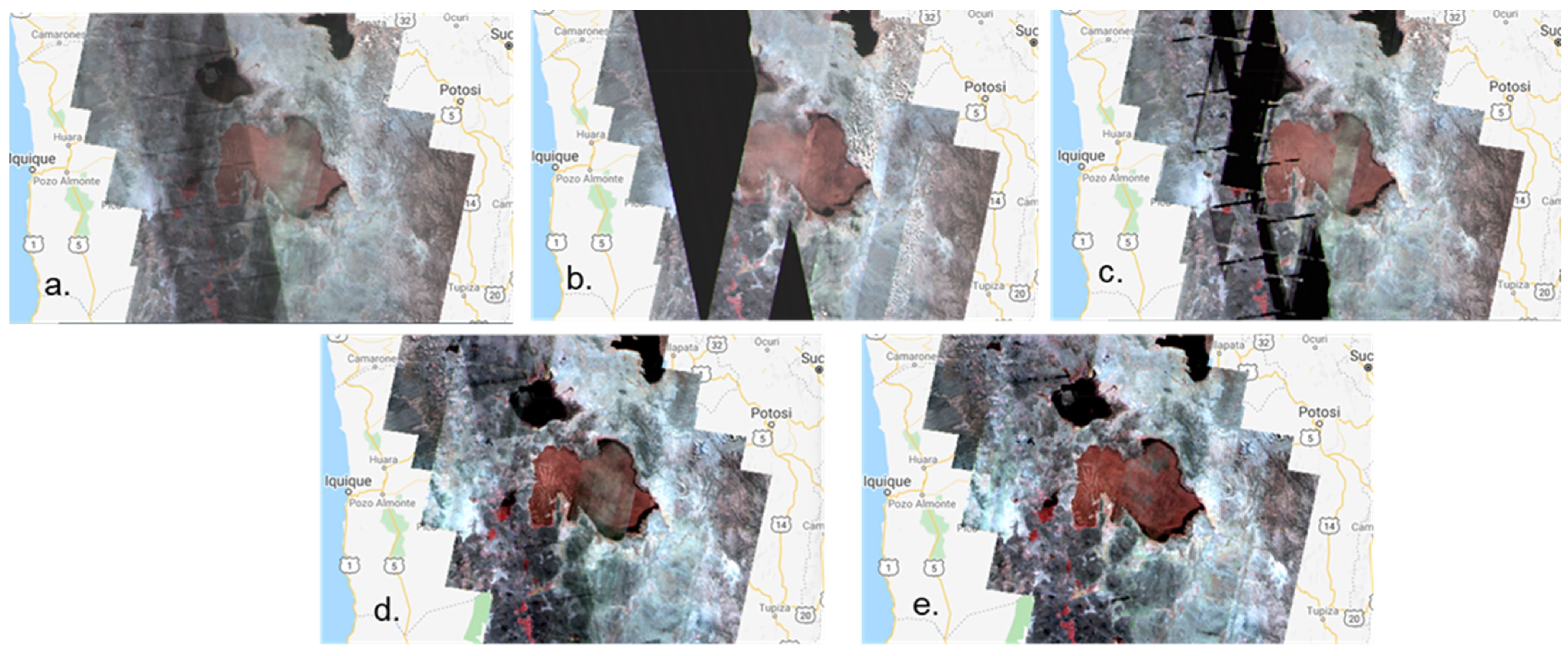
2.2. Remote Sensing Data and Initial Baseline

The framework presented in this study is making use of remote sensing data and auxiliary information taken from existing literature. The data sources and related workflow (geology, hydrogeology, and mass balance) are presented in

Table 1. Datasets used for the study (G = geology, H = hydrogeology, MB = mass balance).

Dataset	Workflow
ASTER	G
Landsat-8	G
SRTM	G
USGS 1:500 k geological map	G, MB
GEOBOL 1:250 k geological maps	G
ERA5	MB
CCI Land Cover	MB
WWF HydroSHEDS	MB
Parameters from available literature (hydrogeology, river flow, Li concentration)	H, MB

. Optical remote sensing data from the ASTER [8] and Landsat-8 [31] missions are employed for the geological processing. A digital elevation model from the SRTM mission [32] is used for the derivation of the river network and the groundwater modelling, in conjunction with WWF HydroSHEDS data [33]. A global land cover map from the Climate Change Initiative [34] is employed for the recharge modelling, alongside meteorological data from the ERA5 re-analysis model [35]. Digital geological map data at a scale of 1:500,000 were obtained from the United States Geological Survey, generalised from primary 1:250,000 scale mapping by geologists from the Servicio Geolgico de Bolivia (GEOBOL) [36]. The digital data were complemented by the use of a subset of the printed 1:250,000 scale GEOBOL maps, which include a more detailed classification of the geological succession and geological profiles showing the vertical relationships and thicknesses [37]. Finally, several parameters necessary to properly develop the workflows are derived from BGS databases and the existing literature [38,39,40]. To be noted, all the input products and parameters are open access in order to preserve the sustainability of the overall framework.

To create a seamless mosaic over the whole study area, ASTER scenes have been composited together within the Google Earth Engine (GEE) platform. ASTER SWIR bands malfunction from April 2008; therefore, combinations of images between 2000 and 2007 have been used. Figure 4 illustrates the challenges in mosaicking ASTER scenes covering the whole study area. In this study, 2000–2001 April to September median imagery has been used for the short-wave Infrared (SWIR) bands (Figure 4e) given the least amount of distortions. The combined distortions from clouds and other scene-related issues are most clearly illustrated by the alternating light and dark bands across the west of the image in Figure 4a. The individual scene edge effects are most obvious in the black patches of Figure 4b,c. Although more subtle, the mean composite image in Figure 4d contains significantly more distortions compared to Figure 4e. For the thermal infrared (TIR) bands, a composite of the mean reflectance of winter months (May to Sep) from 2003 to 2007 offered the most suitable dataset with the least amount of distortions in the TIR.

Minerals exhibit unique absorption and reflection properties in the infrared region of the electromagnetic (EM) spectrum that allow them to be identified, similar to human fingerprints. Whilst iron minerals show characteristic spectral features in the very-near part of the infrared (VNIR), the Al-OH and Fe/Mg-OH bonds of clay minerals show pronounced absorption features in the short-wave infrared. One of the techniques for highlighting the relevant spectral features is through band ratios. Specifically, the Abrams ratio is one of the most widely utilised band ratio for geological mapping in the VNIR–SWIR [41,42,43,44]. Using specific ASTER band naming, the Abrams ratio can be expressed as in Equation (1), where the three channels represent the red, green, and blue image composition. To be noted, the three channels can be seen as proxies for clay, iron oxide, and vegetation. Figure 5a shows the Abrams ratio for the study area.

$$AI\left(R,G,B\right)=\left\{ \frac{B04}{B07},\frac{B03}{B04},\frac{B02}{B01} \right\}$$

(1)

The longer wavelengths in the thermal infrared (TIR) are used for the detection of quartz (SiO₂) and carbonate minerals. Several other indices have been developed in the literature. In this study, we also make use of the Quartz Index (QI), Carbonate Index (CI), and Mafic Index (MI) [7] and combine them in a colour composite image similarly to the Abrams ratio composition in Equation (1). Due to the broad carbonate absorption band at B14 the Mafic Index is sensitive to carbonates, so an adjusted Mafic Index (MIc) has been developed to correct this effect [7]. Figure 5b displays the TIR indices over the study area.

$$QI=\frac{B11*B11}{B10*B12} CI=\frac{B13}{B14} MI=\frac{B2}{B13} MIc=\frac{MI}{CI³}$$

(2)

Finally, the spectral information in the study area is analysed through comparison on a ternary diagram as illustrated in Figure 6. The study area is divided into square polygons of 500 m by 500 m; these polygons are then used to extract the pixel statistics of the overlapping EO data (SWIR and TIR images described in Figure 5) for each polygon. Then, pixel statistics within the polygons are computed and analysed on a ternary plot. The ternary plot created is through the open source library “plotly” in python. This is an interactive tool, which allows hovering over the a point of interest on the graph and understanding which polygon it is through the shapefile ID and its spectral position on the ternary plot.

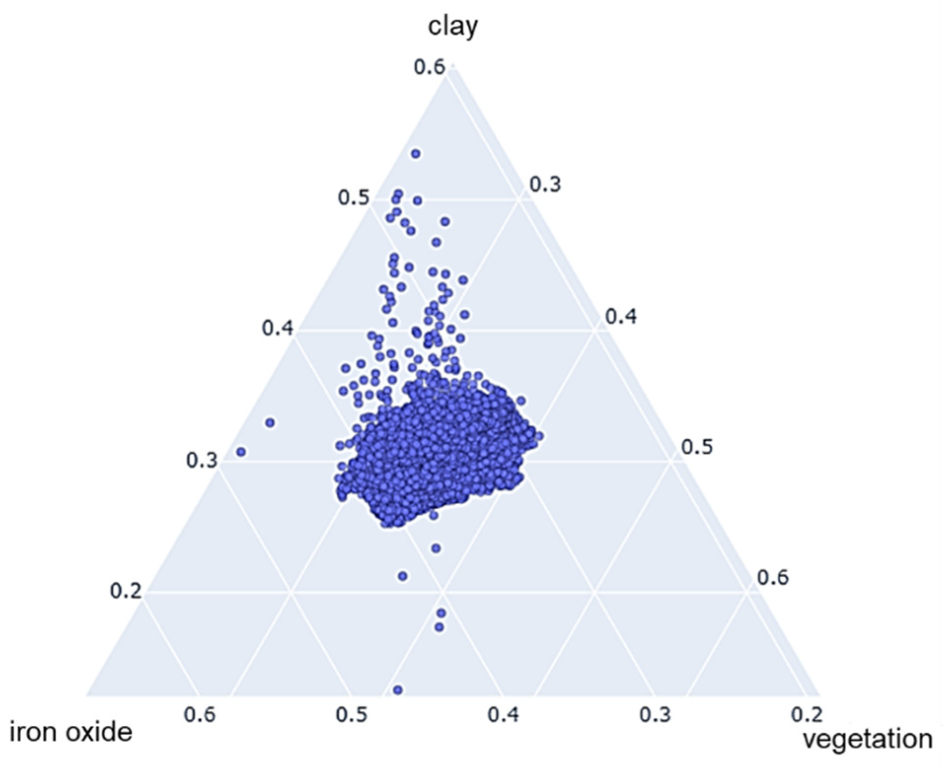
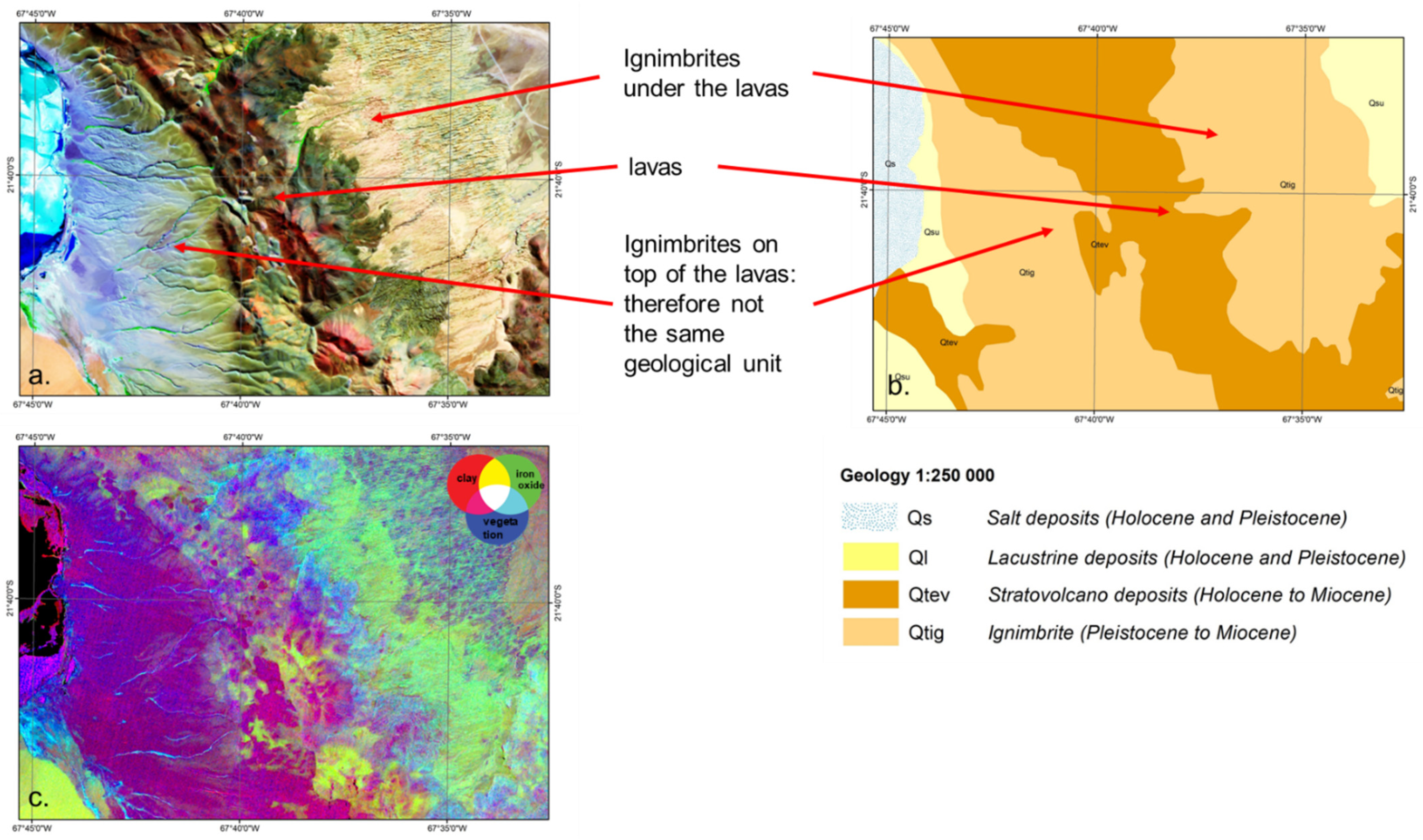
3. Geological Processing

The first stage of the technical framework is the derivation of a conceptual 3D geological model. Determining the three-dimensionality of the geology is important, as the fluid flow and liberation of lithium into the groundwater system takes place both at the ground surface and in the subsurface. Hence, capturing the spatial relationships between the geological units and with the topography allows the vertical ordering and thicknesses of individual units to be inferred of the geology. The model provides a framework that can be used to consider the evolution and movement of lithium-bearing water from source to salar. This was achieved through the integration and interpretation of complementary input datasets including the following: existing digital geological map data and accompanying written explanations, printed geological map data, digital elevation data, and related studies on the local and regional geology [45,46]. The corresponding workflow is depicted in Figure 7. Optical remote sensing data from ASTER and Landsat-8 are used to derive indications of mineral assemblages and underlying lithology as described in Section 2.2. A manual geological interpretation of the EO imagery and derived products and using the input geological map as a starting point is carried out to derive a refined geological map. Geological interpretation in this context uses the spectral and textural information in the imagery and DEMs and the geologist’s knowledge of the geological succession to draw and refine polygons around areas containing the same lithology [7]. Spectral characteristics, as identified in imagery discussed in Section 2, allow areas to be grouped together or separated based on certain characteristics. Ternary plots (Figure 6) are a valuable tool for understanding such similarities; in these, we plot a pixel’s position according to the three bands. Therefore, a predominantly red area in Figure 5a has a higher concentration of clay (red) than iron oxide (green) or vegetation (blue), so it would plot close to the top apex in the ternary plot (Figure 6). In this way we are able to use the ternary plots to identify the areas of superficial sediment which have a similar spectral signature to the lavas or ignimbrites; that is to say, the pixel over the sediment will plot in a similar position on the ternary plot to that from the ignimbrite. Those with a similar signature to the ignimbrites are thought to be primarily derived from the ignimbrites and those with a similar signature to the lavas are thought to be derived from the lavas. These three components allow the assessment of the geological depositional order (as described below) which brings to the final enhanced geological map that covers the entire study area and whose attributes split mapped ignimbrites according to their relative age and subdivides superficial geology based on parent material and hence likely lithium concentrations. In parallel, the river network is derived through geomorphological analysis of the available elevation model [7]. This framework has been exploited for the current test case as described in the following.

The drainage basin for the Salar de Uyuni extends beyond the coverage of the existing geological map data. Therefore, in the first instance, it is necessary to extend the existing 1:500,000 scale geological map to ensure comprehensive coverage of the drainage basin. Specifically, for the hydrological workflow described in the next section, it is important to know all potential sources of lithium that might be mobilised and deposited in the salar. This is accomplished via visual interpretation of a combination of the satellite imagery and derived elevation models. Spectral responses and textural features in the visible and near-infrared parts of the electromagnetic spectrum allow lithological units to be identified on false colour composites of the Landsat-8 and ASTER imagery (Figure 4, Figure 5, and Figure 8a). Existing polygons of the USGS geological map, based on primary surveys that predate the widespread availability of EO data, are then extended using the imagery as a guide. New polygons are created where necessary, and consistent attribution is maintained across the existing and new polygons. Whilst carrying out this remote geological mapping it becomes apparent that some of the existing polygons in the USGS dataset could be modified considering the new satellite imagery and conceptual 3D geological understanding of the project geologists. In these cases, boundaries are adjusted accordingly to create the best geological dataset possible, without visiting the field.

Understanding the geological succession is important to estimate the relative ages of the rock and their spatial relationships, or their relative vertical order or cross-cutting relationship. This can then be linked to the phases of magmatic activity and evolution of the catchment geology, including the distribution of different rock types, which in turn can be linked to the potential amount of lithium in the magmatic system [47]. In the existing geological data, some of the ignimbrites are grouped into a single age. From the relationships observed in the imagery, it is possible to separate the ignimbrites into different relative ages depending on their geometrical relationship to the other ignimbrites and volcanic deposits, including lavas, related to stratovolcanic activity. Figure 8 shows the published geological map (Figure 8b) and a Landsat-8 image (Figure 8a) over a portion of a study area to demonstrate the geological processing workflow. The mapped polygons include two orange polygons representing the same ignimbrite deposit separated by a central brown polygon representing lava flows. Examination of the Landsat-8 image and Abrams ASTER ratio (as described in Section 2.2, Figure 8c) shows that the ignimbrites on to the east appear different in both composition and texture to those in the west. We can also see that the lava flows over the ignimbrites to the east; therefore, the eastern ignimbrites were in place before the lava was extruded and are therefore older. However, the ignimbrites in the west appear to overlap and be on top of the lavas; therefore, the ignimbrites to the west are younger than the lava and as such cannot be the same unit as those in the east. Using this manual interpretation, the geological map was enhanced via the addition and updating of polygon attributes to clearly define the ignimbrites; this was completed over the area of interest and passed to the following workflows.

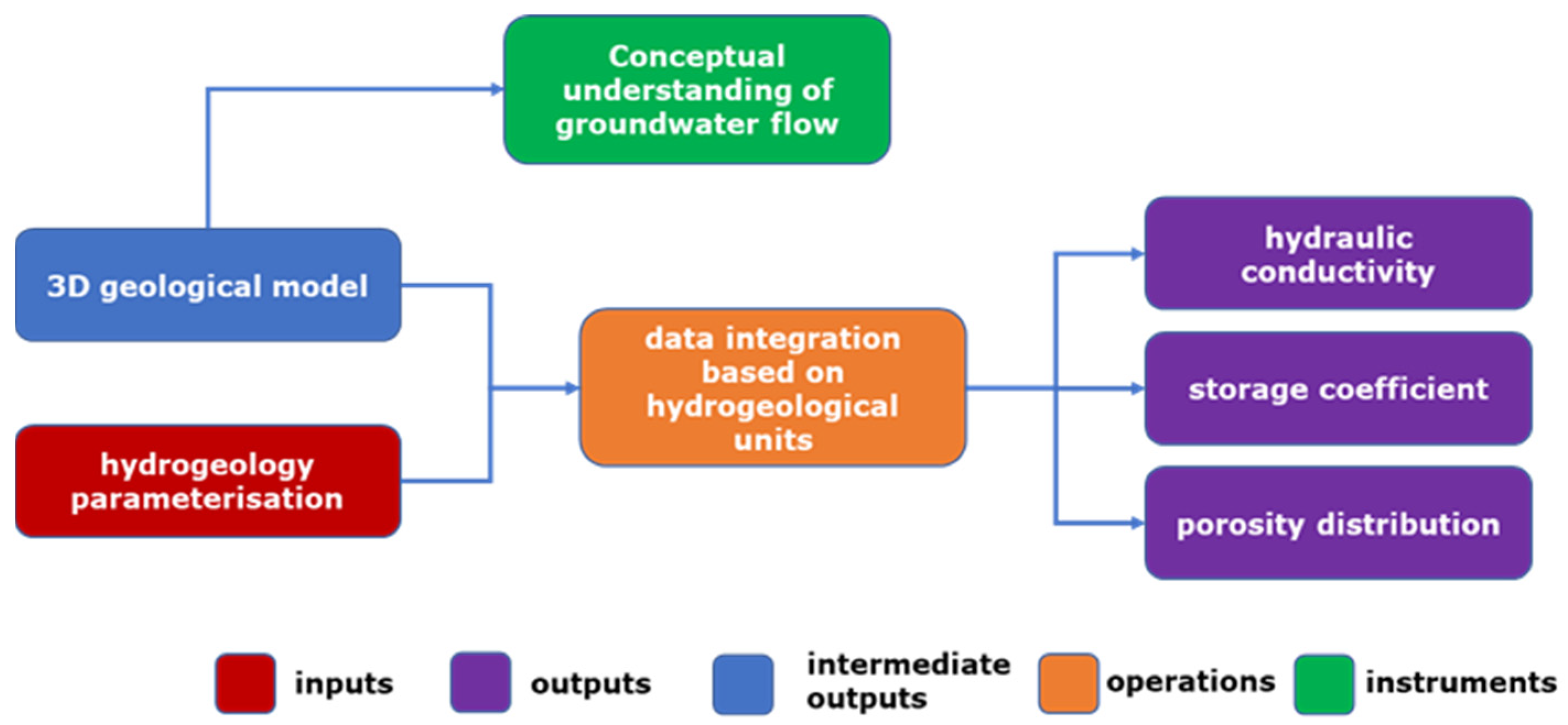
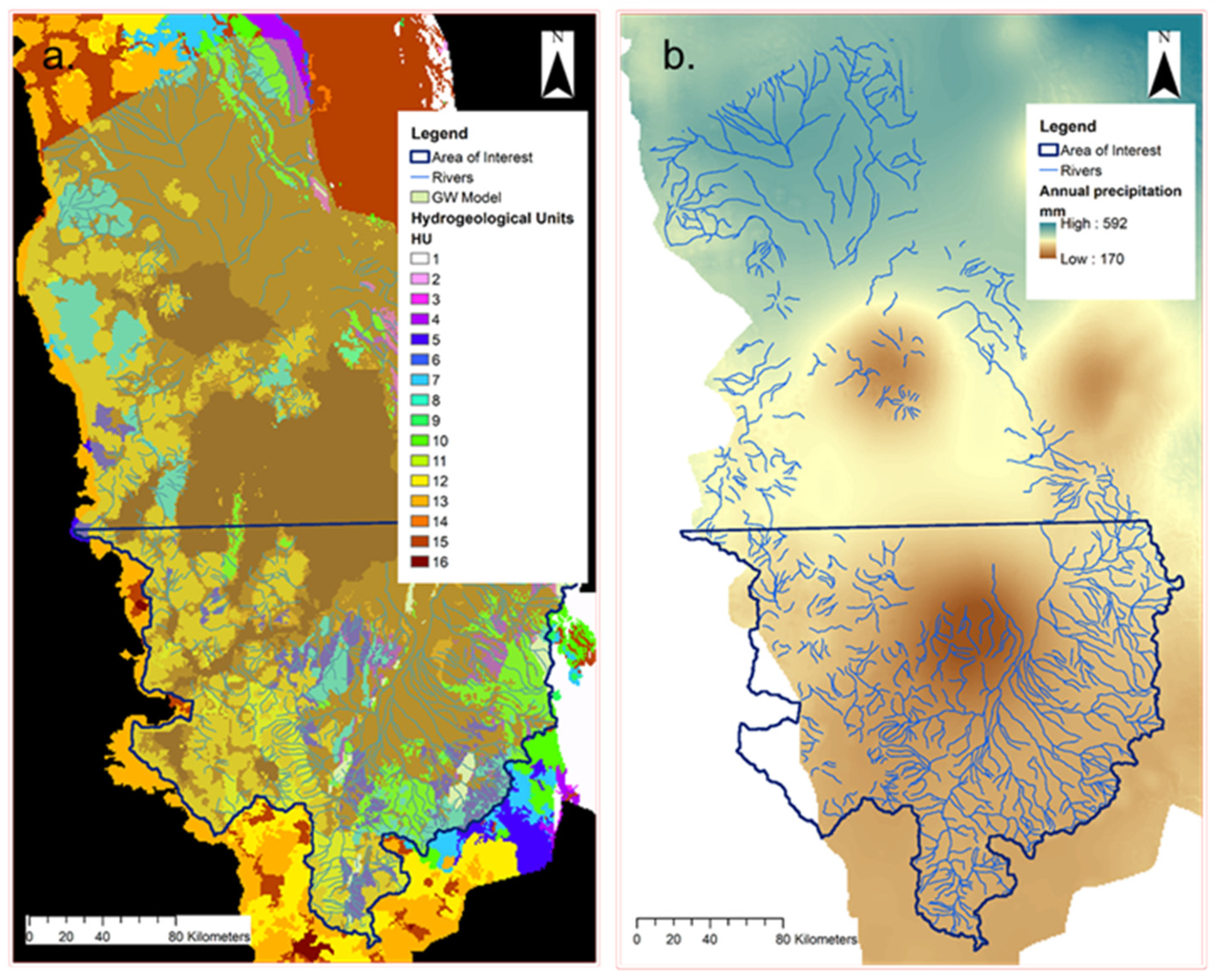
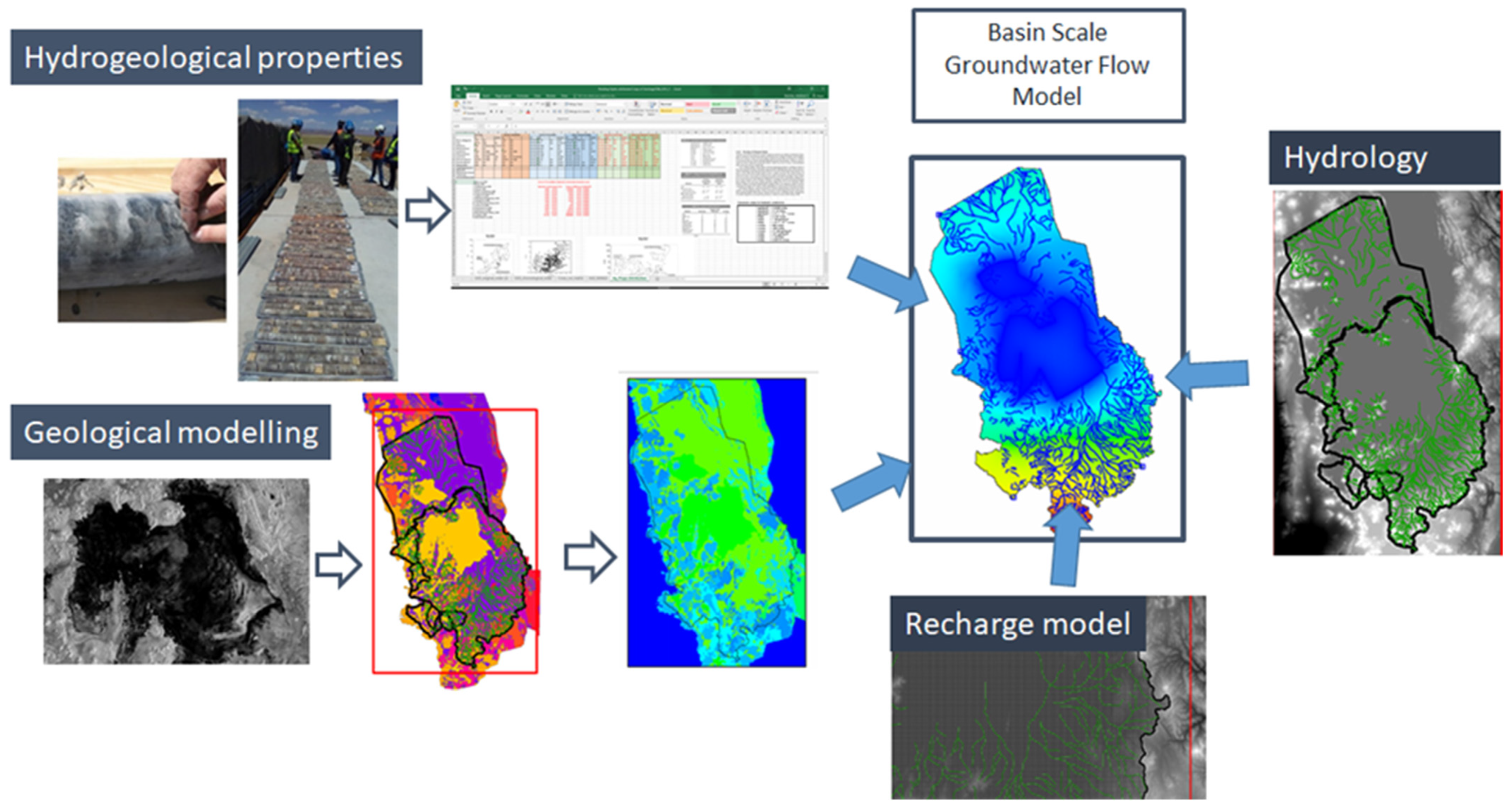
4. Hydrogeological Processing

The second stage of the technical framework is the development of a workflow whereby studied ranges of aquifer properties that control groundwater flow and storage, such as porosity, specific yield, intrinsic and field scale, permeability, hydraulic conductivity, and hence, transmissivity, are constrained. These are attributed to the geological units for the formations encountered in the study area in order to better understand how mineralised water will move. In each case, the data can be refined through ground truthing these properties by field and/or drill core testing either on the salar itself or on the margins or elsewhere in the watershed, and the attributed geology model can then form a hydrogeological attribution model or map. By better understanding the aquifer properties of the formations, one can investigate the hydrochemical processes that can lead to making deposits of particular dissolved elements become valuable resources. Figure 9 shows the relative processing framework. To demonstrate how the workflow can be completed, the initial hydrogeological parameterisation has been derived from BGS data holdings and existing literature, as performed for the current test case [38,39,40]. This was refined as the modelling proceeded to keep the relative values, but the absolute values were adjusted to ensure credible modelling results.

This framework has been exploited for the current test case. The mapping between the geological units and their hydrogeological properties is undertaken by identifying hydrogeological units (HUs). These enable the spatial distribution of the geology either at outcrop for 2D maps or in terms of volumes (3D models) to be attributed. The table in Appendix A illustrates how the 16 lithologies are parametrised based on experience derived from working on other salars and literature values [48]. To be noted, the Geological Description in the table is derived from geo-nsdi.er.usgs.gov/metadata/open-file/95-494/metadata.html (accessed 01 February 2022). In particular, the geology is parametrised using 16 hydrogeological units (HUs; see Appendix A). Each geological unit is given a hydraulic conductivity along with a porosity value. Both are based on experience or background knowledge supplemented by literature values and are used as base variables to feed into the modelling process. These values are then passed to the next and final framework.

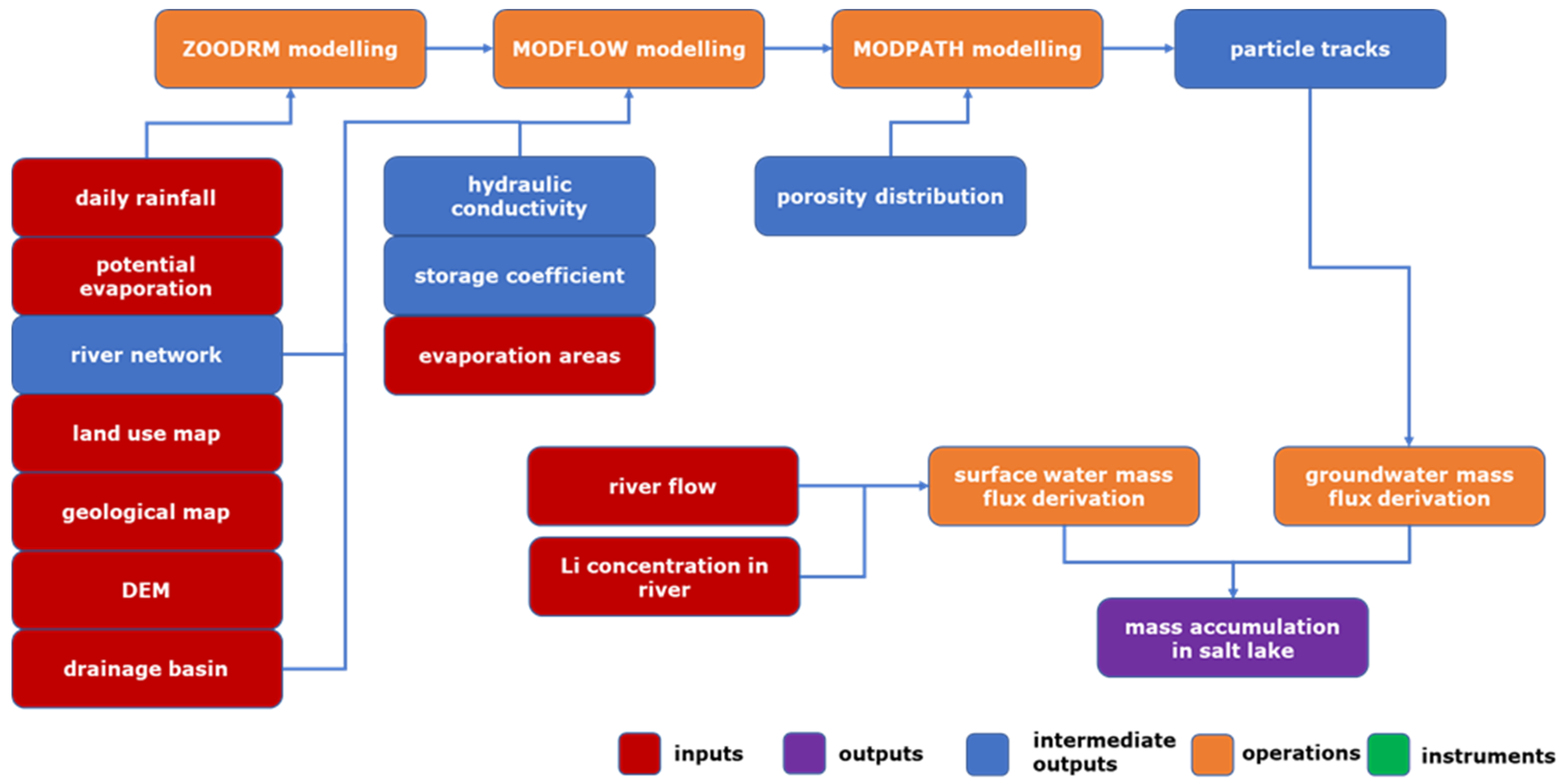
5. Mass Balance Derivation

The final stage of the technical framework has the aim of quantifying the amount of lithium reaching the salar and how long it takes to accumulate. The two methods by which lithium is transported through the watershed are surface water and groundwater. The two are interrelated, with groundwater supplying surface water in the dry season. Therefore, on a long-term basis (~100,000 years [28]), it is necessary to consider how groundwater moves through the system and interacts with the rock mass to leach lithium. To understand the groundwater component, a groundwater flow and particle tracking model of the Uyuni watershed have been developed. These are built on the hydrogeological understanding of the catchment which in turn is built on the geological characterisation. The framework is shown in Figure 10, and it is built on a sequence of processing steps as follows: recharge calculation, e.g., ZOODRM [49]; groundwater flow and velocities, e.g., MODFLOW [50]; and particle tracking, e.g., MODPATH [51]. They take as input several EO products derived in previous stages.

Fluxes from groundwater and surface water masses are computed with the output of the modelling and ground data, respectively. They are required to compute the final mass accumulation in the salt lake. This framework has been exploited for the current test case as described in the following. It is to be noted that the ZOODRM model has not been applied in this case due to the availability of gridded rainfall for Bolivia providing a suitable first guestimate of recharge. It is thought that this method of estimating recharge is commensurate with the complexity of the model and confidence of the other data sources. Once the groundwater model has been developed further and ground-truthed against suitable data such as groundwater heads and baseflow in the rivers, then a more sophisticated approach to calculating recharge can be adopted.

5.1. MODFLOW Model

A steady-state groundwater flow model is developed using the USGS MODFLOW code [50]. The model takes boundary conditions and includes transmissivity (saturated thickness multiplied by hydraulic conductivity), with distributed recharge providing the inflow and outflows based on the rivers and evaporation from the salar itself. The groundwater model and particle tracking model are constructed using a model grid of 1 km in the X and Y directions. The groundwater flow model simulates the movement of water in the subsurface and is based on undertaking a mass balanced for each of the grid cells based on Darcy’s law. The particle tracking model uses mathematical representations of “packets” of water, the particles, to trace the path of groundwater through the system. Alongside this, it enables the time of travel to be calculated, which enables the residence time of the waters in the system to be estimated.

Data inputs are detailed as follows:

• Transmissivity based on a constant 100 m thickness combined with hydraulic conductivity distribution;
• Recharge set to 10% [52] of long-term average rainfall [40];
• Rivers—drain cells based on river network derived from national dataset (World Bank);
• Evaporation based on salar outline.

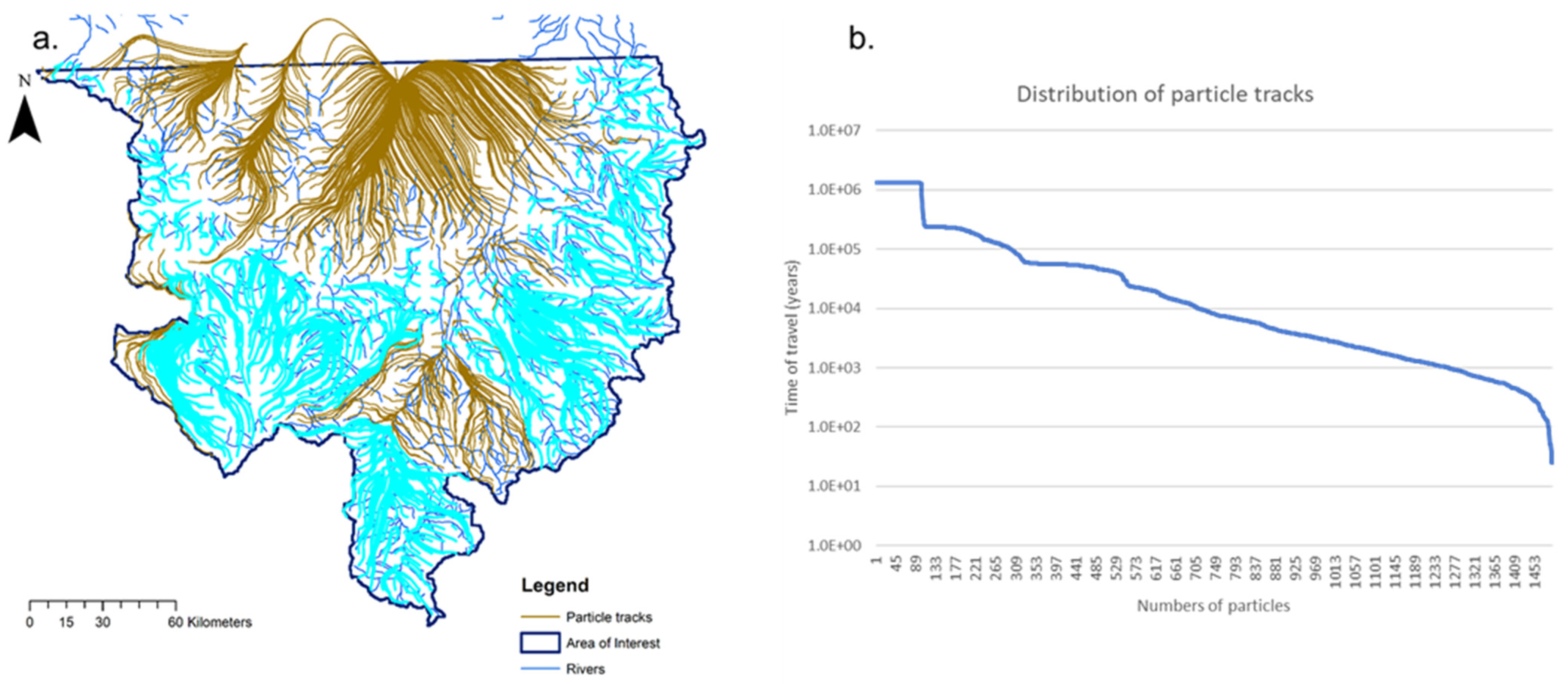
These model features are outlined in Figure 11a,b, and the resulting steady-state groundwater heads are provided in Figure 12. The groundwater heads, which are fluid pressures expressed as heights combined with datum levels, show that the salars in the system act as low points attracting groundwater outflow. The distribution of groundwater heads then approximates the topography, with higher heads in the hinterland surrounding the river valleys and the salars. The initial set of parameters were adjusted so as to ensure that the distribution of groundwater heads was sensible, i.e., not above the ground surface. Further calibration can be undertaken once observed groundwater heads are available. Groundwater flow occurs to the rivers in the base of the valleys and then onto the Salar de Uyuni, reaching it via the main river channel Rio Grande de Lipez.

5.2. MODPATH Model

The MODPATH model (Version 7.2.001) was developed by inheriting most of its data from the MODFLOW model described above. The main extra dataset was porosity based on the zonation from the geology distribution (see Appendix A). The particle tracks were produced for the southern part of the Uyuni watershed developed for the prototype workflow and are shown in Figure 13a. They mainly enter the river system or find their way to the salar itself. The latter is a low point in the system from a groundwater head perspective (see Figure 12) and so will attract any particles that are not captured by the river network. The time distribution of the particles (longest in the system first) is illustrated in Figure 13b. The maximum time of travel is of the order of 1 Ma, consistent with times observed in other salar watersheds, e.g., Atacama [38]. However, the shorter-lived particles (<10,000 a), shown in light blue in Figure 11b, migrate to the rivers where they can flow to the salar via the Rio Grande de Lipez delta [39].

5.3. Mass Balance

The final part of the workflow is the calculation of the mass balance to help understand how the lithium may have accumulated in the salar. This is undertaken by a combination of determining the inflow of lithium mass along with the time groundwater takes to arrive at the salar. The typical concentration of lithium in the main river feeding the salar, Rio Grande de Lipez, is of the order of 1–5 mg/L. Whilst this is low compared to the maximum lithium concentration in the salar of 5–10 g/L, it is relatively high for surface water.

Lithium concentrations in the rock mass within the Uyuni watershed are of the order 16–65 mg/L (see Table 4 in [53]). The groundwaters can then leach lithium and provide input to the river system before it flows into the salar itself in the delta of Rio Grande de Lipez. Previous calculations shown by Risacher and Fritz [39] demonstrate that streamflow inputs estimated at 2 cumecs and lithium concentrations of 3 mg/L can “fill” the salar every 100,000 years. This is a relatively short timescale compared to the time to fill other salars with lithium, e.g., 1.9 Ma for Atacama [38]. However, the particle tracks demonstrate that in the time of travel (~10⁴ years) sufficient lithium can be leached from the rock mass to provide the likely lithium concentrations in groundwaters of the order of 10 mg/L. Given that the particles mainly go to the river system, the concentration observed in the Rio Grande de Lipez can be produced by leaching from rocks in the watershed. Therefore, the workflow enables the current working assumption of a relatively short time to fill the salar with lithium to be realistic. However, considerable uncertainty remains both on the processes as they exist now and the dynamic nature of the system with changes to rock mass and climate. The former can only be addressed with more field data such as groundwater heads and river flows. The latter requires an understanding of geological processes which relies on dating approaches such as geochemical analysis. Nonetheless, the flexibility and repeatability of the workflow enable the calculation to be revisited once more data and understanding become available.

6. Conclusions

In this study, we have developed a complete workflow to characterise the movement of lithium from the watershed into the salt lake. Figure 14 shows the overall conceptual framework, where the groundwater flow and particle tracking models integrate the data workflows. The detailed processing frameworks are shown in Figure 7, Figure 9, and Figure 10, which run sequentially and where the interconnection between frameworks is illustrated by employing the “intermediate output” block which represents an output from a previously run framework. At their hearts is the use of remote sensing data to provide the underpinning datasets. Firstly, remote sensing data feed into the geological modelling (Section 3), which ensures that the geology is as accurate as possible. The extents of geological units are encapsulated in a shapefile which can be ingested in the groundwater flow model. This shapefile is parameterised with hydrogeological properties (Section 4) based on data previously collected on related studies in the region and for similar geological settings. The groundwater flow model is relatively data-hungry (Section 5) and amongst other data requires input from a recharge model. The recharge model, which is itself data-intense, relies on rainfall and potential evaporation data, along with land use, DEM, and the drainage or river network. The extent of the models is defined by the basin boundary. The outflow from the recharge model is fed into the groundwater flow model which along with the parametrised geology and the river network can be used to set up the groundwater flow model. The output from the groundwater flow model is used to drive the particle tracking model in conjunction with the porosity distribution, which is again derived from the geology. Appendix B details the data requirements to build the framework. The models are then used to determine both surface and groundwater flow paths in the basin and how water–rock interaction can allow the waters to pick up lithium and then bring it into the salar. Whilst lithium has accumulated in the salar over the long timescales, this is difficult to simulate as both the rock mass and the climate vary over this time period. For example, the region is subject to wetter and drier periods on the cyclicity of 10,000 years [39]. Further, the groundwater inflows to the salar may not be recharged contemporaneously; rather, they may have been built up during wetter periods and are only now finding their way to the salar [52]. This is borne out by the timescales predicted by the modelling, albeit with uncertainties associated with simulating processes over such long timescales.

The workflow is flexible and can be used with different model codes as well as simpler approaches, such as distributed rainfall rather than a fully featured recharge model. Whilst the workflow presented here is an example based on open data sources, measurements can and should be used to validate the approach. However, given the extent of open data sources available, the workflow demonstrates how far it is possible to go with freely available data. Given the open approach, uncertainty can be addressed in a number of different ways. Firstly, choosing and swapping out different components of the workflow can be used to assess how differing data sources affect the outcome. Secondly, the ease by which the process can be reproduced can enable sensitivity analysis to be undertaken. Finally, the availability of the workflow enables independent assessment and scrutiny of the process and its outcome. The outputs from this study have been benchmarked against previous work undertaken in the Uyuni watershed as well as other studies in salars in the Lithium Triangle countries, e.g., Atacama.

References

1. Hund, K.; La Porta, D.; Thao, P.; Tim, L.; John, D. Minerals for Climate Action: The Mineral Intensity of the Clean Energy Transition; World Bank Group Report; World Bank: Washington, DC, USA, 2020. [Google Scholar]
2. USGS. Lithium: Mineral Commodity Summary; USGS: Reston, VA, USA, 2021.
3. USGS. Lithium: Mineral Commodity Summary; USGS: Reston, VA, USA, 2011.
4. Munk, L.A.; Hynek, S.A.; Bradley, D.C.; Boutt, D.; Labay, K.; Jochens, H. Lithium Brines: A Global Perspective. Rev. Econ. Geol. 2016, 18, 339–365. [Google Scholar]
5. Flexer, V.; Celso Fernando, B.; Claudia, I. Lithium recovery from brines: A vital raw material for green energies with a potential environmental impact in its mining and processing. Sci. Total Environ. 2018, 639, 1188–1204. [Google Scholar] [CrossRef] [PubMed]
6. Barandiarán, J. Lithium and development imaginaries in Chile, Argentina and Bolivia. World Dev. 2019, 113, 381–391. [Google Scholar] [CrossRef] [Green Version]
7. Gupta, R. Remote Sensing Geology; Springer: Berlin/Heidleberg, Germany, 2017. [Google Scholar]
8. Yamaguchi, Y.; Kahle, A.; Tsu, H.; Kawakami, T.; Pniel, M. Overview of advanced spaceborne thermal emission and reflection radiometer (ASTER). EEE Trans. Geosci. Remote Sens. 1998, 36, 1062–1071. [Google Scholar] [CrossRef] [Green Version]
9. Marghany, M.; Mazlan, H. Lineament mapping using multispectral remote sensing satellite data. Int. J. Phys. Sci. 2010, 5, 1501–1507. [Google Scholar] [CrossRef]
10. Masoud, A.; Katsuaki, K. Auto-detection and integration of tectonically significant lineaments from SRTM DEM and remotely-sensed geophysical data. ISPRS J. Photogramm. Remote Sens. 2011, 66, 818–832. [Google Scholar] [CrossRef]
11. Rajan, G.; Sundararajan, M. Mapping of mineral resources and lithological units: A review of remote sensing techniques. Int. J. Image Data Fusion 2019, 10, 79–106. [Google Scholar] [CrossRef]
12. Pour, A.; Hashim, M.; Park, Y.; Hong, J.K. Mapping alteration mineral zones and lithological units in Antarctic regions using spectral bands of ASTER remote sensing data. Geocarto Int. 2018, 33, 1281–1306. [Google Scholar] [CrossRef]
13. Sabins, F. Remote sensing for mineral exploration. Ore Geol. Rev. 1999, 14, 157–183. [Google Scholar] [CrossRef]
14. Van der Meer, F.; van Ruitenbeek, F.J.A.; van der Werff, H.; Noomen, M.F.; van der Meijde, M.; Hecker, C.A.; Carranza, E.J.M.; de Smeth, B.; Woldai, T. Multi-and hyperspectral geologic remote sensing: A review. Int. J. Appl. Earth Obs. Geoinf. 2012, 14, 112–128. [Google Scholar] [CrossRef]
15. Waters, P.; Greenbaum, D.; Smart, P.L.; Osmaston, H. Applications of remote sensing to groundwater hydrology. Remote Sens. Rev. 1990, 4, 223–264. [Google Scholar] [CrossRef]
16. Singhal, B.; Ravi, P. Applied Hydrogeology of Fractured Rocks; Springer Science & Business Media: Berlin/Heidelberg, Germany, 2010. [Google Scholar]
17. Cardoso-Fernandes, J.; Teodoro, A.C.; Lima, A.; Perrotta, M.; Roda-Robles, E. Detecting Lithium (Li) mineralizations from space: Current research and future perspectives. Appl. Sci. 2020, 10, 1785. [Google Scholar] [CrossRef] [Green Version]
18. Cardoso-Fernandes, J.; Teodoro, A.C.; Lima, A. Remote sensing data in lithium (Li) exploration: A new approach for the detection of Li-bearing pegmatites. Int. J. Appl. Earth Obs. Geoinf. 2019, 76, 10–25. [Google Scholar] [CrossRef]
19. Santos, D.; Teodoro, A.; Lima, A.; Cardoso-Fernandes, J. Remote Sensing Techniques to Detect Areas with Potential for Lithium Exploration in Minas Gerais, Brazil. In Proceedings of the SPIE, SPIE Remote Sensing, Strasbourg, France, 9–12 September 2019. [Google Scholar]
20. Gemusse, U.; Lima, A.; Teodoro, A. Comparing Different Techniques of Satellite Imagery Classification to Mineral Mapping Pegmatite of Muiane and Naipa: Mozambique. In Proceedings of the SPIE, SPIE Remote Sensing, Strasbourg, France, 9–12 September 2019. [Google Scholar]
21. Rossi, C.; Spittle, S.; Bayaraa, M.; Pandey, A.; Henry, N. An Earth Observation Framework for the Lithium Exploration. In Proceedings of the IGARSS 2018—2018 IEEE International Geoscience and Remote Sensing Symposium, Valencia, Spain, 22–27 July 2018. [Google Scholar]
22. Winograd, I.; William, T. Hydrogeologic and Hydrochemical Framework, South-Central Great Basin, Nevada-California, with Special Reference to the Nevada Test Site; USGS: Washington, DC, USA, 1975.
23. Fricker, H.A.; Minster, B.; Carabajal, C.; Quinn, K.; Bills, B.; Borsa, A. Assessment of ICESat performance at the salar de Uyuni, Bolivia. Geophys. Res. Lett. 2005, 32. [Google Scholar] [CrossRef] [Green Version]
24. Rossi, C.; Rodriguez Gonzales, F.; Fritz, T.; Yague-Martinez, N.; Eineder, M. TanDEM-X calibrated raw DEM generation. ISPRS J. Photogramm. Remote Sens. 2012, 73, 12–20. [Google Scholar] [CrossRef]
25. Brown, T.J.; Idoine, N.E.; Wrighton, C.E.; Raycraft, E.R.; Hobbs, S.F.; Shaw, R.A.; Everett, P.; Deady, E.A.; Kresse, C. World Mineral Production 2015–2019, BGS. 2019. Available online: https://www2.bgs.ac.uk/mineralsuk/download/world_statistics/2010s/WMP_2015_2019.pdf (accessed on 1 February 2022).
26. Rettig, S.L.; Jones, B.F.; François, R. Geochemical evolution of brines in the Salar of Uyuni, Bolivia. Chem. Geol. 1980, 30, 57–79. [Google Scholar] [CrossRef]
27. Risacher, F.; Hugo, A.; Carlos, S. The origin of brines and salts in Chilean salars: A hydrochemical review. Earth-Sci. Rev. 2003, 63, 249–293. [Google Scholar] [CrossRef]
28. Risacher, F.; Fritz, B. Origin of Salts and Brine Evolution of Bolivian and Chilean Salars. Aquat. Geochem. 2008, 15, 123–157. [Google Scholar] [CrossRef]
29. Hofstra, A.H.; Todorov, T.I.; Mercer, C.N.; Adams, D.T.; Marsh, E.E. Silicate melt inclusion evidence for extreme pre-eruptive enrichment and post-eruptive depletion of lithium in silicic volcanic rocks of the western United States: Implications for the origin of lithium-rich brines. Econ. Geol. 2003, 105, 1691–1701. [Google Scholar] [CrossRef]
30. Godfrey, L.; Álvarez-Amado, F. Volcanic and saline lithium inputs to the Salar de Atacama. Minerals 2020, 10, 201. [Google Scholar] [CrossRef] [Green Version]
31. Roy, D.P.; Wulder, M.A.; Loveland, T.R.; Woodcock, C.E.; Allen, R.G.; Anderson, M.C.; Helder, D.; Irons, J.R.; Johnson, D.M.; Kennedy, R.; et al. Landsat-8: Science and product vision for terrestrial global change research. Remote Sens. Environ. 2014, 145, 154–172. [Google Scholar] [CrossRef] [Green Version]
32. Van Zyl, J.J. The Shuttle Radar Topography Mission (SRTM): A breakthrough in remote sensing of topography. Acta Astronaut. 2001, 48, 559–565. [Google Scholar] [CrossRef]
33. Wickel, B.A.; Lehner, B.; Sindorf, N. HydroSHEDS: A Global Comprehensive Hydrographic Dataset. In AGU Fall Meeting Abstracts; Center for Astrophysics: Cambridge, MA, USA, 2007; Volume 2007. [Google Scholar]
34. Li, W.; MacBean, N.; Ciais, P.; Defourny, P.; Lamarche, C.; Bontemps, S.; Houghton, R.A.; Peng, S. Gross and net land cover changes in the main plant functional types derived from the annual ESA CCI land cover maps (1992–2015). Earth Syst. Sci. Data 2018, 10, 219–234. [Google Scholar] [CrossRef] [Green Version]
35. Hoffmann, L.; Günther. G.; Li, D.; Stein, O.; Wu, X.; Griessbach, S.; Heng, Y.; Konopka, P.; Muller, R.; Vogel, B.; et al. From ERA-Interim to ERA5: The considerable impact of ECMWF’s next-generation reanalysis on Lagrangian transport simulations. Atmos. Chem. Phys. 2019, 19, 3097–3124. [Google Scholar] [CrossRef] [Green Version]
36. Sherman, P.; Richter, D.H.; Ludington, S.; Soria-Escalante, E.; Escobar-Diaz, A. Digital Geologic Map of the Altiplano and Cordillera Occidental, Bolivia, United States Geological Survey; Open-File Report 95–494; U.S. Department of the Interior: Washington, DC, USA, 1995.
37. Departamento Nacional de Geologia (DNG). Sheet 6234 Rio Mulatos; Departamento Nacional de Geologia, Ministerio de Minas y Petroleo: La Paz, Bolivia, 1962.
38. Munk, L.A.; Boutt, D.F.; Hynek, S.A.; Moran, B.J. Hydrogeochemical fluxes and processes contributing to the formation of lithium-enriched brines in a hyper-arid continental basin. Chem. Geol. 2018, 493, 37–57. [Google Scholar] [CrossRef]
39. Risacher, F.; Fritz, B. Geochemistry of Bolivian salars, Lipez, southern Altiplano: Origin of solutes and brine evolution. Geochim. Cosmochim. Acta 1991, 55, 687–705. [Google Scholar] [CrossRef]
40. VVicente-Serrano, S.; Kenawy, A.; Azorin-Molina, C.; Chura, O.; Trujillo, F.; Aguilar, E.; Martín, N.; Lopez-Moreno, I.; Sanchez-Lorenzo, A.; Morán-Tejeda, E.; et al. Average monthly and annual climate maps for Bolivia. J. Maps 2015, 12, 295–310. [Google Scholar] [CrossRef] [Green Version]
41. Abrams, M.J.; Rothery, D.A.; Pontual, A. Mapping in the Oman ophiolite using enhanced Landsat Thematic Mapper images. Tectonophysics 1988, 151, 387–401. [Google Scholar] [CrossRef]
42. Abrams, M.; Yamaguchi, Y. Twenty years of ASTER contributions to lithologic mapping and mineral exploration. Remote Sens. 2019, 11, 1394. [Google Scholar] [CrossRef] [Green Version]
43. Amer, R.; Kusky, T.; Ghulam, A. Lithological mapping in the Central Eastern Desert of Egypt using ASTER data. J. Afr. Earth Sci. 2010, 56, 75–82. [Google Scholar] [CrossRef]
44. Mia, B.; Fujimitsu, Y. Mapping hydrothermal altered mineral deposits using Landsat 7 ETM+ image in and around Kuju volcano, Kyushu, Japan. J. Earth Syst. Sci. 2012, 121, 1049–1057. [Google Scholar] [CrossRef] [Green Version]
45. Baker, M.C.W. The nature and distribution of upper Cenozoic ignimbrite centres in the Central Andes. J. Volcanol. Geotherm. Res. 1981, 11, 293–315. [Google Scholar] [CrossRef]
46. Salisbury, M.; Jicha, B.R.; de Silva, S.L.; Singer, B.S.; Jimenez, N.C.; Ort, M.H. 40Ar/39Ar chronostratigraphy of Altiplano-Puna volcanic complex ignimbrites reveals the development of a major Magmatic Province. Geol. Soc. Am. Bull. 2011, 123, 821–840. [Google Scholar] [CrossRef]
47. Ort, M.H.; De Silva, S.L.; Jiménez, C.N.; Jicha, B.R.; Singer, B.S. Correlation of ignimbrites using characteristic remanent magnetization and anisotropy of magnetic susceptibility, Central Andes, Bolivia. Geochem. Geophys. Geosystems 2013, 14, 141–157. [Google Scholar] [CrossRef] [Green Version]
48. Houston, J.; Butcher, A.; Ehren, P.; Evans, K.; Godfrey, L. The evaluation of brine prospects and the requirement for modifications to filing standards. Econ. Geol. 2011, 106, 1225–1239. [Google Scholar] [CrossRef] [Green Version]
49. Mansour, M.M.; Wang, L.; Whiteman, M.; Hughes, A.G. Estimation of spatially distributed groundwater potential recharge for the United Kingdom. Q. J. Eng. Geol. Hydrogeol. 2018, 51, 247–263. [Google Scholar] [CrossRef] [Green Version]
50. Harbaugh, A.W. MODFLOW-2005, the US Geological Survey Modular Ground-Water Model: The Ground-Water Flow Process; US Department of the Interior, US Geological Survey: Reston, VA, USA, 2005; pp. 6–16.
51. Pollock, D.W. User Guide for MODPATH Version 6: A Particle Tracking Model for MODFLOW; US Department of the Interior, US Geological Survey: Reston, VA, USA, 2012; p. 58.
52. Boutt, D.F.; Corenthal, L.G.; Moran, B.J.; Munk, L.; Hynek, S.A. Imbalance in the modern hydrologic budget of topographic catchments along the western slope of the Andes (21–25° S): Implications for groundwater recharge assessment. Hydrogeol. J. 2021, 29, 985–1007. [Google Scholar] [CrossRef]
53. Davis, J.R.; Howard, K.A.; Rettig, S.L.; Smith, R.L.; Ericksen, G.E.; Risacher, F.; Morales, H.A.R. Progress Report on Lithium-Related Geologic Investigations in Bolivia; USGS: Washington, DC, USA, 1982.
Figure 1. (a) Aerial view of lithium ponds at the Salar de Uyuni, Bolivia (© contains modified Copernicus Sentinel data (2017), processed by ESA, CC BY-SA 3.0 IGO); (b) view across the ponds, of about 1 km width (© UK Research and Innovation (UKRI)/British Geological Survey (BGS)).
Remotesensing 14 01383 g001
Figure 2. Location (a) and extension of the area of interest (AoI) over the Salar de Uyuni in Bolivia (b). Basemap images copyright © 1995–2020 Esri.
Remotesensing 14 01383 g002
Figure 3. Schematic illustration of the salar and catchment, showing potential sources of lithium (weathering of volcanic bedrock and derived sediments) in the upper part of the drainage basin, coinciding with areas of higher precipitation; pathways for surface water and groundwater flow that transports lithium from source areas to the salar (blue lines); and the salar where lower precipitation and higher evaporation result in the concentration of inflowing water to create lithium-enriched brines. Other potential sources of lithium exist, including direct input from hydrothermal sources (red lines).
Remotesensing 14 01383 g003
Figure 4. Different approaches to compositing ASTER scenes: (a) 2000–2006 May–September mean; (b) 2000–2006 May–September mosaic; (c) 2000–2006 May–September median; (d) 2000–2001 April–September mean, scene footprints visible; (e) 2000–2001 April–September median.
Remotesensing 14 01383 g004
Figure 5. Spectral index maps developed over the study area. (a) SWIR Abrams ratio. RGB image channels are clay (R), iron oxide (G), and vegetation (B). (b) TIR index combination. RGB image channels are Quartz Index (QI) (R), Carbonate Index (CI) (G), and Mafic Index corrected (MIcor) (B).
Remotesensing 14 01383 g005
Figure 6. Polygon spectra of “IRG” units on ternary plot. Spectra from Abrams ratio image with 3 bands representing clay, iron oxide, and vegetation.
Remotesensing 14 01383 g006
Figure 7. Geological processing workflow.
Remotesensing 14 01383 g007
Figure 8. Geological interpretation aided with EO data over a portion of the study area. The general temporal relationship is indicated by the legend (Qs, youngest, to Qtig, oldest; see Appendix A for details); however, the geological interpretation shows that multiple instances and ages of Qtig (ignimbrite) occur, including relatively young ignimbrite deposits (western part of the map) and relatively old ignimbrite deposits (eastern part of the image), separated by an intervening unit of stratovolcano deposits. (a) Landsat-8 RGB colour composite topographically shaded; (b) geological map; (c) Abrams ASTER ratio.
Remotesensing 14 01383 g008
Figure 9. Hydrogeological processing framework.
Remotesensing 14 01383 g009
Figure 10. Mass balance framework.
Remotesensing 14 01383 g010
Figure 11. MODFLOW modelling. (a) Model setup with HUs (see Appendix A), model extent, and rivers; (b) long-term average rainfall.
Remotesensing 14 01383 g011
Figure 12. MODFLOW modelling output. Steady-state groundwater heads.
Remotesensing 14 01383 g012
Figure 13. MODPATH and mass balance outputs: (a) particle tracks (104 years and younger are highlighted in light blue) and (b) time of travel distribution for area of interest.
Remotesensing 14 01383 g013
Figure 14. Conceptual framework.
Remotesensing 14 01383 g014