Article

What Can We Learn from Nighttime Lights for Small Geographies? Measurement Errors and Heterogeneous Elasticities

1
Institute of Macroeconomics, Leibniz University Hannover, 30167 Hannover, Germany
2
Department of Political Science, University of California San Diego, 9500 Gilman Drive #0521, La Jolla, CA 92093, USA
3
School of Global Policy and Strategy, University of California San Diego, 9500 Gilman Drive #0519, La Jolla, CA 92093, USA
*
Author to whom correspondence should be addressed.
Remote Sens. 2022, 14(5), 1190; https://doi.org/10.3390/rs14051190
Submission received: 27 December 2021 / Revised: 11 February 2022 / Accepted: 21 February 2022 / Published: 28 February 2022
(This article belongs to the Special Issue Remote Sensing of Night-Time Light)

Abstract

:
Nighttime lights are routinely used as a proxy for economic activity when official statistics are unavailable and are increasingly applied to study the effects of shocks or policy interventions at small geographic scales. The implicit assumption is that the ability of nighttime lights to pick up changes in GDP does not depend on local characteristics of the region under investigation or the scale of aggregation. This study uses panel data on regional GDP growth from six countries, and nighttime lights from the Defense Meteorological Satellite Program (DMSP) to investigate potential nonlinearities and measurement errors in the light production function. Our results for high statistical capacity countries (the United States and Germany) show that nightlights are significantly less responsive to changes in GDP at higher baseline level of GDP, higher population densities, and for agricultural GDP. We provide evidence that these nonlinearities are too large to be caused by differences in measurement errors across regions. We find similar but noisier relationships in other high-income countries (Italy and Spain) and emerging economies (Brazil and China). We also present results for different aggregation schemes and find that the overall relationship, including the nonlinearity, is stable across regions of different shapes and sizes but becomes noisier when regions become few and large. These findings have important implications for studies using nighttime lights to evaluate the economic effects of shocks or policy interventions. On average, nighttime lights pick up changes in GDP across many different levels of aggregation, down to relatively small geographies. However, the nonlinearity we document in this paper implies that some studies may fail to detect policy-relevant effects in places where lights react little to changes in economic activity or they may mistakenly attribute this heterogeneity to the treatment effect of their independent variable of interest.

1. Introduction

A growing literature in economics and other fields uses nighttime lights as a proxy for economic activity when data on gross domestic product (GDP or GDP per capita) are unavailable. Nightlights have been used to compare economic activity across geographic units at a variety of scales, from seminal work at the country level [1,2,3], over states/provinces [4], down to the level of cities [5], villages [6,7], and grid cells [2]. An increasingly common application of nightlights is to measure regional or local economic impacts of shocks (such as floods [8], sanctions [9], or transportation cost shocks [5]) or spatially-targeted policies (such as a rural employment scheme [10], federal transfers to a state [11], or regional favoritism by political leaders [4]). However, little is known about whether the nightlights-GDP relationship at smaller geographic scales is constant across locations. Note that while we focus on the relationship between nightlights and GDP, other studies have used survey data to study the correlation with income or income proxies when GDP data are unavailable [6,12,13]. Beyond GDP, nightlights have been used to as a proxy for population density [7,14], electrification [15], and infrastructure [16].
Interpreting how changes in nightlights reflect unmeasured changes in economic activity requires having a reliable estimate from settings where both nightlights and economic activity are measured. Recent work has explored how the relationship between growth in nightlights and economic activity varies across contexts, both at national scale [17] and at smaller geographies [7]. Some studies conclude that the subnational nightlights-GDP relationship is not stable in emerging and advanced economies [18]. Others find that luminosity is ineffective as a proxy for economic activity in less densely populated counties in the United States and may be a poor predictor of GDP in areas where agriculture plays a crucial role in the economy [19]. Given that physical features underlying economic activity usually vary by economic sector (across agriculture and industry, for example) and by population density, it seems plausible that the relationship between changes in nightlights and economic growth varies across contexts. However, it is often overlooked that the presence of measurement errors in nighttime lights and GDP complicates the interpretation of such findings and makes it difficult to separate the influence of measurement errors from heterogeneity in the data generating process. As a result, little is known about how stable this relationship is at finer levels of spatial disaggregation and what this potential heterogeneity might imply for studies using nightlights as a proxy for economic activity. Unfortunately, this raises the potential of incorrect inference regarding the economic effects of a policy, investment or shock. If, for example, nightlights are not associated with changes in economic activity over some range of GDP or population density, then a policy intervention or public investment in these kinds of areas might be incorrectly labeled as ineffective if researchers estimate its economic impacts solely through nightlights. Similarly, variation in the nightlights-GDP relationship might lead researchers to conclude that a policy had heterogeneous impacts on economic activity across locations, even when the true economic impact does not vary.
This paper makes three contributions. First, we compile subnational economic data from several high and middle income countries together with data on nighttime lights and discuss the sources of measurement errors in both. Second, we estimate the nightlights-GDP elasticity—the percentage change in nightlights associated with a one percent change in economic activity—in two different ways: (i) unconditionally for different income groups to gauge whether the relative attenuation factors consistent with a constant elasticity are plausible, and (ii) by conditioning the elasticity on population density. Our results illustrate significant nonlinearity at subnational scale. The estimated elasticities tend to fall with higher levels of GDP, higher population densities, and the size of the agricultural sector. We find that the required variation in measurement errors would have to be implausibly large and follow an improbable pattern to explain these findings, which implies that the structural elasticity likely varies. Finally, we study changes in the nightlights-output relationship at various configurations of geographic aggregation. We find that the average relationship and the evidence in favor of nonlinearity is remarkably stable across geographies of different shapes and sizes, even though the influence of measurement errors in lights and GDP should decrease as units become larger. Simultaneously, the variation of estimates around the average increases as the number of units falls. Given the previous evidence, this suggests that in addition to sampling variation, spatial correlation in industrial composition and population density contributes to this pattern.

2. Materials and Methods

Applied researchers typically use nighttime lights as a proxy for GDP when data on income or production are unavailable. In the canonical regression equation setup, GDP would be on the left hand side, if it were observed, and some policy intervention or other variable of interest on the right hand side. The researcher is interested in the treatment effect of the policy on GDP. Replacing GDP by nighttime lights (whether as a sum or density per unit area) implies that the policy parameter of interest is not statistically identified. Instead, the researcher obtains a product of the policy effect on GDP, say τ , multiplied by the elasticity of nighttime lights with respect to GDP, say β . To see this, let the policy equation of interest be y i G = τ d i + e i while the structural relationship between lights and GDP is y i L = β y i G + ϵ i , where y G is GDP, y L is nighttime light output and d i is the variable for the policy being evaluated. Both quantities are in logs and could be measured in per capita terms. Since GDP is not observed, the researcher actually estimates y i L = θ d i + ϵ i . In this case, it is straightforward to show that the probability limit of θ ^ is β τ . This is precisely why the literature typically multiplies the policy parameter by an estimate of the inverse elasticity of lights with respect to GDP, in order to relate their estimates back to changes in aggregate income [3]. The elasticity of lights with respect to output is typically assumed to be constant. In fact, usually an estimate of 0.3 [3,4] is used in order to back out the effect of the policy on GDP. However, if there is heterogeneity in how nightlights react to GDP, then this has an important implication: any systematic variation in the elasticity of nightlights with respect to GDP will translate into differences in the estimated effect of the policy across locations, even when the true effect of the policy is constant.
Unfortunately, both nighttime lights and GDP data are subject to measurement error. The DMSP nighttime lights that are used in most of the literature suffer from four sources of error: (1) bottom-coding as a result of filtering and limited detection of low lights, (2) topcoding as a result of sensor saturation in bright areas, (3) blooming or overglow as a result of atmospheric scattering and “pollution” from adjacent light sources, exacerbated by geolocation errors, and (4) a lack of inter-annual calibration which makes it impossible to convert the recorded digital numbers into a physical quantity such as radiance [5,20,21,22,23]. Moreover, as we discuss below, measuring subnational GDP in all countries often involves assumptions about the location of certain economic activity, or interpolations of baseline year surveys for industrial or agricultural output conducted infrequently [24]. GDP data in developing countries are particularly error-prone and could be subject to outright manipulation [25]. The presence of measurement error on both sides of the equation has long been recognized in the economics literature focused on estimating the relationship between nighttime lights and GDP, or optimal combinations of both [2,3,17,26].
The newer VIIRS day-night band solves many of the legacy technology issues of the DMSP system. The sensor has a smaller ground footprint, better ability to detect lights at both ends of the spectrum, and is radiometrically calibrated. This paper focuses on DMSP for two reasons. First, most applications of nightlights in economics research have used DMSP given the longer time series (VIIRS data are only available from 2012 onward, resulting in short panels with GDP). Second, VIIRS satellites observe nighttime lights much closer to midnight when most production and consumption have ceased. Nevertheless, evidence suggests that the VIIRS data vastly outperforms the DMSP system when it comes to predicting GDP [19]. While the number of studies using VIIRS is undoubtedly on the rise, we use the DMSP data in this analysis to speak to the existing literature and leave a similar exercise with VIIRS for future work.
In our setting, the key implication of measurement error in both variables is that we cannot simply take estimates obtained from regressions on subsamples, or nonlinear regressions, at face value and definitively conclude that there is nonlinearity in the structural elasticity. Differences in the elasticity could be due to structural differences in how light reacts to GDP (e.g., higher densities in cities combined with economies of scale in light use or differential light consumption by different economic sectors) or due to differences in measurement error (e.g., due to greater informality or difficulty measuring the activity of some regions). To circumvent this issue, we calculate how large the measurement error would need to be in order to fully explain the observed variation in the elasticity. We can then ask if the implied measurement error is plausible in countries where we expect these errors to be small and constant across units, and then use these estimates to assess the variation in countries where measurement errors should play a larger role. We study what the literature calls the structural relationship (how lights react to GDP), as opposed the predictive relationship (how lights predict GDP), but make no attempt to estimate the structural relationship net of measurement error. Other work focuses on the country level and proposes a method of identifying the elasticity under the presence of very general forms of measurement error using proxies for the statistical capacity of each country [17]. We use subnational data where variation in statistical capacity is not helpful for identification.
Our article examines the nightlights-GDP relationship in Brazil, China, Germany, Italy, Spain and the United States, spanning a range of quality in national accounts (and by extension subnational accounts) in order to gauge variation in the structural relationship in both higher and lower measurement error contexts. In addition, these countries are large and diverse in terms of their geography and economic structure, have subnational GDP data available for a suitable number of years, and have a large number of second-level administrative units (county/municipality/district) to ensure sufficient statistical power for estimation. These countries also vary in terms of quality grades for their national accounts, which we take as a proxy for the quality of their subnational accounts. For example, if we take quality grades from the 1994 Penn World Table 5.6 and 2008 Penn World Table 6.1 in order to reflect data quality during years corresponding to our study period, then the United States and Germany have an A grade, Italy an A−, Spain a B+, Brazil a B and China a C [27,28].

2.1. Empirical Strategy

We study the potential heterogeneity in the income elasticity of lights across subnational units using two different but related approaches. Both take the constant elasticity model underlying most of the applied literature as the benchmark and then set up different conditions which would lead us to reject this model. We focus on GDP (as opposed to other measures such as GDP per capita) because the economics literature studying the relationship between nightlights and economic activity or employing nightlights as a proxy focuses on GDP instead of GDP per capita. The implicit assumption is that growth in nighttime lights increases equally in population growth and growth in per capita incomes. Secondly, GDP per capita is not always positively correlated to total economic activity.
First, we specify single variable regressions of the observed nighttime lights ( y i t L ) on GDP per area ( y i t G ), both in logarithms, for samples split according to quartiles of average GDP. More formally, for each subsample we specify
y i t L = β y i t G + μ i + ψ t + ϵ i t
where μ i and ψ t represent geographic unit and year fixed effects, respectively, and ϵ i t is an idiosyncratic error.
Together with the specification in logarithms, the inclusion of unit fixed effects implies that we are relating a region’s growth in nighttime lights to growth in GDP. The inclusion of time fixed effects allows for country-specific factors that vary over time but influence every administrative unit in the same way (such as differences in the ability of sensors to pick up nighttime lights, due to satellite changes or orbital or sensor degradation). We are therefore estimating the relationship of changes in nightlights and economic activity within a geographic unit over time, and not how the level of nightlights is associated with economic activity across geographic units. This is the relevant estimation to inform empirical exercises studying the impact of a shock, policy or investment at subnational level.
Our parameter of interest, β , is the income elasticity of nighttime lights, a unitless measure indicating the percentage luminosity increase in response to a one percent change in GDP. We estimate this parameter separately for subsamples split according to quartiles of average GDP to obtain four coefficients ( β ^ k for k = 1 , 2 , 3 , 4 ). These four groups of different average GDP are a proxy for subnational differences in statistical capacity. Under the conditional mean independence assumptions typically made in the related literature [2,3,26] the resulting estimates will converge to the true coefficient times an attenuation factor. If the true relationship were constant across all subsamples of the data and the variance of the measurement error in GDP were constant, then the estimated elasticities should be very similar in each partition of the data (with some expected sampling variation). More formally, β ^ k p β λ . If the true relationship is constant but the GDP error variance differs across subsamples, then the estimated coefficients will be attenuated differently, such that β ^ k p β λ k . In this case, it is plausible that the highest GDP category would have the smallest measurement error in GDP, resulting in the least attenuation of the coefficient. However, our analysis does not presume any particular pattern of attenuation. Appendix A derives these results and provides details on the required assumptions.
We use this relationship to study whether the differences in elasticities and the implied attenuation factors are plausible. If the true structural elasticity is assumed constant, the ratio of any two point estimates indicates how different measurement errors must be in order explain the variation in the estimated elasticities across the two subsamples. For each country, we estimate and report the ratios θ k = β k / β 1 comparing the quarter k to the data up to the first quartile. If, for example, the variance of measurement errors in GDP falls with higher incomes, then the sequence of coefficient estimates would be rising and we would interpret a ratio of, say, θ ^ 4 = 0.5 / 0.25 as ‘the income elasticity of nighttime lights has to be twice as attenuated in the lowest GDP quartile than the highest GDP quartile for the constant elasticity model to be true’. The pattern would be reversed if the variance of measurement errors in GDP increases with income. If we cannot reject the hypothesis that the ratio is different from one, then we conclude that their attenuation factors could have been the same.
Going one step further, we interpret values of θ k statistically different from 1 in countries with high statistical capacity as evidence against the constant elasticity model typically assumed in the applied literature. Of course, it is plausible that the variation in measurement errors of subnational GDP is substantial in developing countries, where there may be more variation in informality across regions, or in the capacity of the statistical apparatus to collect economic data. However, in developed countries with uniformly high statistical capacity, we should not observe significant differences in the signal-to-noise ratio of GDP across regions, and, in fact, expect the estimated θ ^ s to be close to one. Even if the signal-to-noise ratio in the best measured part of the data were, say, 0.8, then a doubling or halving of this ratio for some regions would imply implausibly large differences in measurement error in high capacity countries. This is why our sample of countries deliberately spans highest quality subnational accounts (the US or Germany) and countries where regional GDP is estimated with less precision (China or Brazil). We use the estimates from developed economies to better understand the relative roles of “structural” nonlinearities and measurement errors in the light-output relationship in developing economies, where nighttime lights are most often used as a proxy for local GDP.
Note that our assumptions measurement errors in GDP and lights also imply that the standard errors of the estimated coefficients are biased. While the sign is indeterminate, it can be shown that the resulting t-statistics are underestimated. The standard errors of the estimated relative attenuation factors are also affected by measurement errors. We leave potential solutions to these issues for future research and note that our estimates of the uncertainties are not free of large sample biases.
Our second approach to studying heterogeneity in the income elasticity models the variation along a third variable:
y i t L = ( β + γ z i ) y i t G + μ i + ψ t + e i t = β y i t G + γ ( y i t G z i ) + μ i + ψ t + ϵ i t
where z i is the logarithm of population density in the first year of the data and all other variables are defined as before. We focus on population density since the light-GDP relationship could vary along this dimension for several reasons. For example, fixed costs of light infrastructure can be large at low population densities, while at high densities, economies of scale and vertical city growth may decrease the responsiveness of lights to changes in GDP.
Given that both light and GDP per area are in logarithms, taking the derivative of Equation (2) with respect to y i t G results in an elasticity that varies with initial population density. For this specification, we are no longer interested in ratios of these elasticities at different points in the distribution but instead focus on the sign and significance of γ ^ . It is important to note that all coefficient estimates in specifications with multiple independent variables, of which at least one is measured with error, are biased in unknown directions. However, if we are willing to assume that population density in the initial year is measured without error and make additional independence and linearity assumptions, then γ ^ converges to zero in probability if the constant elasticity model is correct (see Appendix A for details on these results). Moreover, β ^ will still be attenuated by the same signal-to-noise ratio as in Equation (1). Hence, we may compare the estimates of β ^ across the long and short regressions and, with some caveats, interpret a significant result on γ ^ as further evidence against the constant elasticity model.
Another likely source of structural differences in the nightlight-economic output relationship are differences in industrial composition. For example, if nighttime lights fail to pick up changes in agricultural GDP [29,30], then differences in sectoral composition across regions are sufficient to generate variation in the measured light-output relationship. Given that agricultural areas are typically less densely populated than regions with large manufacturing or service hubs, this would also imply some variation of the light-output elasticity with respect to population density. Moreover, it is an open question whether lights primarily respond to value-creation in industry or services and whether the elasticity is constant within each economic sector. Light in densely populated urban areas with a high concentration of services, for example, might not scale linearly in output. To explore this in our data, we run regressions of nightlights on GDP separately for agricultural, industry (including construction), and service sector GDP, with and without interactions with population density. Just as with aggregate output, we cannot simply compare the coefficients for different sectors to gauge whether structural elasticity varies because measurement errors are likely to vary across sectors. Instead, maintaining the same assumption from above, we again ask if the implied relative measurement errors are plausible and check whether the interaction with population density is significant.
Finally, we analyze whether aggregation to geographic units of different shapes and sizes changes the pattern of the resulting estimates. This may occur for two reasons related to our analytical framework. First, aggregating smaller units to larger units could reduce measurement errors in both GDP and lights. For example, county GDP errors due to downscaling state data or workplace versus place of residence mismatches are offset when small regions are grouped together. Similarly, overglow of nightlights into neighboring regions becomes internalized when analyzing larger areas, and the relative importance of topcoding decreases as the size of units increases. A second reason for why aggregation could affect the pattern of elasticities is the grouping of smaller units (with potentially different structural elasticities) into larger, more economically mixed units. Regardless, assessing how geographic scale affects the observed elasticities can help explain the disparate findings documented in the literature, which typically finds large variation in elasticities across countries and across different levels of aggregation within the same country [18,19].
Previous research on the Modifiable Areal Unit Problem (MAUP) in urban economics suggests that size and shape of administrative units matters little in comparison to other specification issues but also finds that aggregating to large units can distort the underlying relationship [31]. No study has systematically examined this problem in the context of nighttime lights and GDP.
We use methods from the literature on the MAUP [31,32] to study whether the design of regions creates variation in sectoral composition and population density, which, in turn, generates differences in the structural nightlights-economic output relationship. Specifically, we use disaggregated data on local GDP for the continental United States (3080 counties) and Brazil (5569 municipalities) to create many alternative administrative divisions of varying shapes and sizes. We construct simulated partitions for a given number of administrative units, k, using the following random-seed-and-grow algorithm [31]. We start out with the finest level of aggregation into n units. First, we randomly pick one seed unit. Second, we identify the unit’s closest neighbor before merging these two units so that now there are n 1 units remaining. We repeat these steps until n = k . The resulting partition is geographically contiguous. We run the algorithm 1000 times for every 200th number of units from k ̲ = 50 to some country-specific maximum k ¯ . We take 50 as a lower bound since this is the number of US states and then simulate the result for k { 50 , 200 , 400 , 600 , , k ¯ } , where k ¯ is 3000 for the US and 5400 for Brazil. This results in thousands of alternative divisions of the Unites States and Brazil over which we can aggregate nighttime lights, GDP and population, and estimate the specifications given in Equations (1) and (2). A persistence of nonlinearity in simulations with high levels of aggregation (where measurement errors become less severe) would provide additional evidence that the structural elasticity varies.

2.2. Data

We compile data on subnational GDP, sectoral composition, and population from a variety of sources. For each country, Table 1 lists the smallest geography for which subnational GDP data are available, the number of units, years for which the data are available, the industrial classification used (if available), and the primary source. We deflate current local currency units by the national GDP deflator from the World Development Indicators if the data are not provided in real (constant price) quantities. In the case of the U.S. and European countries, we compute the GDP in each industrial sector by aggregating all NAICS or NACE sectors to a three-sector classification (agriculture, manufacturing and construction, and services). We also obtain high-quality vector geometries representing the geographical units within each country from national statistical offices or other public databases. Data for China is not widely available, which is why we use GDP (in USD) for 299 prefectures from the Economist Intelligence Unit and supplemented this data with information from annual yearbooks and the CEIC’s China Economic Database for the 30 missing prefectures, four municipalities and nine county-level cities.
Measuring economic activity at small geographic scale can be challenging in any country. In addition to the usual data collection and processing errors that arise for national accounts, subnational accounts are particularly prone to non-statistical errors. These include imputations, conceptual differences, index construction, sectoral definitions, and the scope of the exclusions (such as home production, subsistence farming, illegal activity and smuggling) [33]. Often, subnational estimates of GDP require triangulating with multiple data sources, or downscaling data collected for higher-level administrative regions. This is true even in high statistical capacity countries. In the United States, the Bureau of Economic Analysis relies on the income approach to measure GDP at state and county level, computed as the sum of compensation of employees, taxes on production and imports minus subsidies, and gross operating surplus (capital income). This method has the potential to underestimate capital-intensive industries whose production relies heavily on physical or financial capital [34]. It measures GDP at people’s place of work, as opposed to place of residence. Interpolation between benchmark years and downscaling from state-level data introduce other sources of measurement error. For example, years when the Economic Census is available (every 5 years) are used as benchmark years, with other years interpolated using sales data from the National Establishment Time Series (NETS) database. In addition, some state-level data on OIC (income payments other than employees and proprietors) are distributed among counties using NETS, the Quarterly Census of Employment and Wages (QCEW), Economic Census data, and industry-specific data from various sources [35].
Similar methodological challenges exist in the European Union, although analysis on revisions suggest that estimation errors are small (when countries undergo revisions they constitute less than 1% of GDP). However, there are likely to be larger errors in the historical series. Regional GDP is calculated as regional Gross Value Added plus taxes on products minus subsidies. GVA, in turn, is calculated using the production approach (value of output minus intermediate inputs) or the income approach (similar to the U.S.) depending on the member state [36]. Ongoing work in the European Union is tackling methodological questions for regional GDP such as recording foreign direct investment, non-market services, incorporating global production and integrated global accounts, the digital economy and other price and volume measures for intellectual property products [37,38].
Less is known about the quality of subnational accounts in Brazil and China. Brazilian municipal GDP is based on Gross Value Added calculated at state level with the production approach, where state GDP is distributed among municipalities using various methods depending on the good or service [39]. China officially uses both the production and income methods for national accounts; value-added of agriculture, forestry, animal husbandry and fishery is calculated by the production method, while the current value-added of other industries is calculated using the income method. Regional GDP is measured by local governments using the production approach from major surveys on large industrial firms, large service sector firms, and some construction firms. These data are supplemented by surveys of smaller firms and administrative data from government departments. In addition, they estimate expenditure by household surveys and investment project surveys. Since local Chinese governments are rewarded for meeting growth targets, the Chinese National Bureau of Statistics revises local GDP estimates in computing national GDP [40,41].
We obtain nighttime lights within each geography from 1992 until 2013 from the Defense Meteorological Satellite Program (DMSP) Operation Line Scan (OLS) sensors. Specifically, we use annual composites which report yearly average “stable lights” as a 6-bit digital number (DN) from 0 to 63, after observations affected by cloud cover, background noise and other disturbances have been removed. We follow common practice to delete gas flares from the annual composites. Gas flares are disproportionately bright in relation to the change in output they represent and create significant overglow into neighboring pixels. Like Henderson et al. [3], we also set all pixels that are not on land to zero. For each region-year pair, we calculate the sum of lights and total area of all pixels. Our outcome of interest is the logarithm of lights per area (ln DN/km 2 ). Table 2 provides the distribution of nightlight density values across subnational regions by country.
Physical detection limits of the DMSP sensors and the difficulty of separating background noise and transient lights from permanent light sources effectively impose a bottom-coding threshold where pixels with DNs of 1–2 and small clusters of pixels with values of less than 4 DN are removed in the stable lights composite. Solutions to this problem range from adding the minimum detection threshold to recorded lights in a region [5] to using auxiliary data to distinguish background noise from “human lights” [42]. The problem is most severe in Sub-Saharan Africa, where a lack of consistent electrification implies that mid-sized settlements can be missed. Rural electrification rates are close to 100% in Brazil and China today—the two emerging economies in our data—so we consider this source of error to be less important in our study than others. In fact, very few observations record zero light (see Table 2).
A potentially serious issue in subnational analyses is that the DMSP data are heavily topcoded. Topcoding primarily occurs in city centers as the sensor gradually reach its saturation limit and affects values well below 63 DN in the yearly averages [21,23]. The intensity of topcoding is correlated with our variables of interest, such as average GDP, density, and industrial structure. To deal with this issues, one of our tests uses topcoding corrected data [23] which applies a Pareto-correction to the stable lights composites (and builds on the radiance-calibrated data available in selected years [21]).
The DMSP data exhibit overglow or blurring effects for a variety of reasons. The nominal resolution of the data provided by the National Centers for Environmental Information (NCEI) is 30 arc seconds. However, the effective instantaneous field of view (EIFOV) expands from 2.2 km to about 5.4 km at the edge of the scan and the system “smoothes” these data on-board by forming pixel blocks that are 2.7 km by 2.7 km (with different location offsets for each nightly image [22]). As a result, the same light source will show up in several 30 arc second pixels. On-board processing also magnifies the blur effect for brighter light sources [22]. Geolocation errors which displace lights by about 3 km exacerbate this problem [20]. We discuss the biases introduced by overglow within administrative units when presenting the results and allow for spatial correlation across units in a robustness check.
A final challenge in using the DMSP data is that the recorded DN cannot be mapped to a physical quantity (radiance). This occurs because the sensors dynamically adjust their low-light detection ability over the lunar cycle but the sensor’s ‘variable gain’ settings are not stored [21]. Efforts have been made to calibrate using light emitted from islands (such as Sicily) and using active targets for some nights [43]. However, there are simply no permanently constant light sources on Earth that can unequivocally solve this problem in the historical data, while ad hoc calibration adjustments have the potential to introduce more noise. Another source of variability across years is that the orbit of the DMSP satellites slowly degrades over time, recording lights at a slightly earlier time each day. This feature has recently been used to extend the DMSP data from 2012 to 2019 using pre-dawn data from older satellites that crossed back into a dawn-dusk orbit [44]. We do not use the extended series as the orbital shift to pre-dawn hours introduces an additional source of measurement error. Following the economics literature [3], we average the data whenever two years are available and include year fixed effects in all regressions. This accounts for differences in average sensor settings in each year which affect all regions in the same manner. If all pixels were illuminated and topcoding did not exist, then a constant shift in each year would fully account for this problem. However, since differences in gain settings also imply that some pixels cross the detection threshold and others become topcoded before on-board averaging occurs, there is likely to be some residual region-year specific error which cannot be accounted for.
As motivation, Figure 1 illustrates the raw correlations between light density and economic density. We observe a strong degree of nonlinearity whenever the correlation is based on highly disaggregated data (as in the case of US counties, municipalities in Brazil, and, to a lesser extent, districts in Germany) and less nonlinearity when the data are more aggregated (provinces and prefectures in Italy, Spain and China).

3. Results

3.1. Analysis of Estimates by Income Group

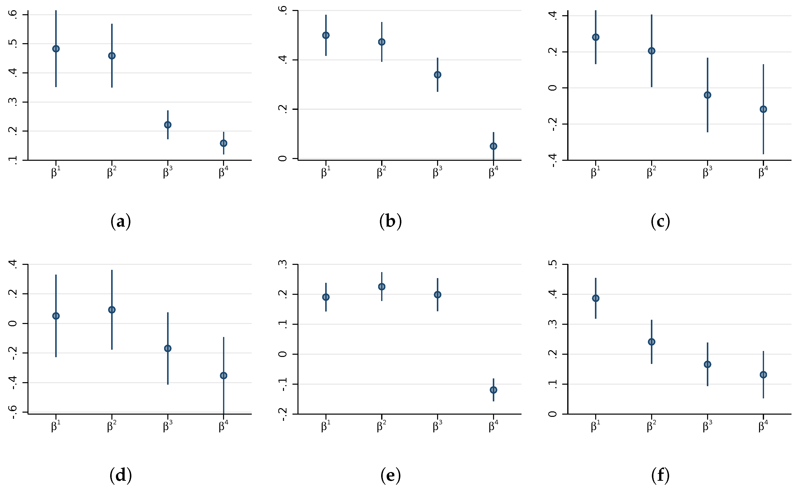
We begin by investigating potential heterogeneity in the light-output relationship using regressions estimated on samples split according to quartiles of average GDP. For each country in our data set, Figure 2 shows the estimated income elasticities of nightlights using four equal-sized groups of the data, with β 1 referring to the coefficient for regions up to the lowest GDP quartile, and β 4 for the regions above the highest quartile.
The results in Figure 2a,b show the patterns for the U.S. and Germany, the countries with the highest statistical capacity in our sample. Rather than estimates which are constant or rise with average incomes, we observe the highest elasticities among regions in lowest quartile ( β ^ 1 = 0.482 for the United States and β ^ 1 = 0.499 for Germany) followed by a steady decline as we move up in the distribution of average incomes which matches the raw correlations presented in Figure 1. In fact, the estimates for the group with the highest incomes are either approaching zero in the case of the United States ( β ^ 4 = 0.158 ) or cannot be distinguished from zero in the case of Germany ( β ^ 4 = 0.050 ). Of course, the presence of measurement errors implies that we cannot take this evidence at face value. However, it is difficult to rationalize this pattern with measurement errors alone since it implies that the errors in GDP would have to be increasingly severe as incomes rise if the constant elasticity model were correct.
Figure 2c,d report the results for Italy and Spain which, like Germany, use EU reporting standards but had somewhat lower statistical capacity and a larger informal sector in the 1990s. For Italy, the estimated elasticities are lower at every split of the data (consistent with greater attenuation throughout) but they also show a decreasing pattern as incomes rise. For Spain, we find elasticities that are indistinguishable from zero for the first two GDP quartiles and even negative in the highest quartile. While some of the lack of statistical significance is likely due to having few cross-sectional units for Italy and Spain, the pattern is consistent with the findings for the United States and Germany.
Figure 2e,f present the estimates for the two emerging economies in our data set where measurement error in GDP likely plays a larger role. The estimates for Brazil suggest that the relationship is approximately constant (with estimates around 0.2) until we reach the highest quartile of aggregate income (where we estimate a negative elasticity of −0.119). Somewhat remarkably, the estimates for Chinese prefectures follow the same decreasing pattern of the US counties or German districts, and even have comparable magnitudes ( β ^ 1 = 0.386 and β ^ 4 = 0.132 ).
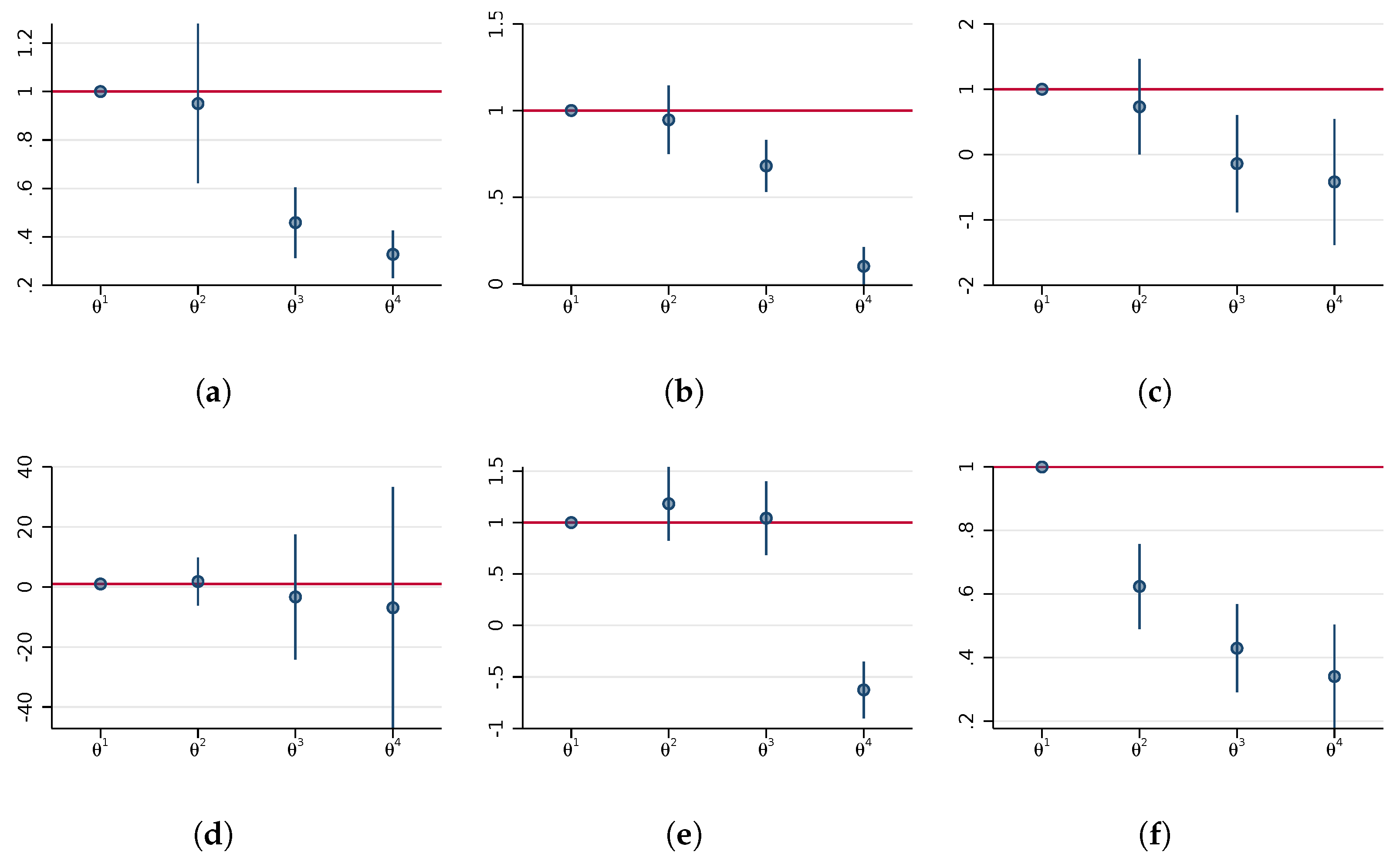
Figure 3 plots the implied relative attenuation effects and their 95% confidence intervals, or more specifically, the ratio of the coefficient ( β k ) estimated for each GDP quartile to the coefficient estimated in the data up to the first quartile ( β 1 ). The first ratio θ 1 is equal to one by construction, and we are interested in substantively large and statistically significant deviations from one in the other three quarters of the data.
Figure 3a,b show the results for the United States and Germany. As a result of the similar coefficient estimates up to the median of average GDP, we find no evidence suggesting that the signal-to-noise ratios differ in these two quarters of the data (see θ ^ 2 s). However, we estimate large differences the more we move up in the distribution of average GDP. For the United States, the coefficient in the third (fourth) GDP quarter would need to be more than two (three) times as attenuated as the coefficient estimated up to the first GDP quartile. For Germany, the ratio of coefficients in the third to the first quartile implies that the former is about 1.5 times more attenuated than the latter, while our estimate of θ ^ 4 is about 0.1, suggesting that the coefficient in the highest quartile is 10 times more attenuated than that of the lowest quartile if the structural elasticity were truly constant. Given the high quality of the GDP data in these two countries and the fact that we have sufficient units in each group to estimate the uncertainties of these ratios relatively precisely, we consider these implied differences in measurement errors across income groups too large to be plausible. We are not aware of studies suggesting that such differences in measurement errors across subnational units are likely, especially since regional accounts in the United States and Germany are developed by a single federal authority (the Bureau of Economic Analysis for United States and the Federal Statistical Office of Germany). Moreover, the suggested pattern of increasing measurement error with higher incomes appears unlikely. Instead, these results strongly suggest that the structural elasticity declines as GDP rises.
Figure 3c–f repeat this exercise with data from Italy, Spain, Brazil and China. The estimates for Italy and Spain also suggest that measurement errors rise with GDP but the confidence interval of these ratios are comparatively wide. For Italy the upper bound of the 95% confidence intervals for θ ^ 4 is 0.546 and the confidence intervals for Spain always include one. We find near constancy in Brazil up to the third quartile but then the estimate of θ ^ 4 falls below zero which cannot be meaningfully interpreted in terms of relative attenuation factors that are theoretically bounded by zero from below. The estimates for China mirror the results for the United States and Germany. They suggest that if the constant elasticity model were correct, measurement errors would have to be strictly increasing in average GDP. Moreover, the coefficient in the highest quarter would have to be close to three times more attenuated than that in the first.
An important robustness check, given that we observe this decreasing pattern of elasticities, is whether these differences are simply driven by topcoding in the lights data. If topcoding is severe, then changes in GDP do not translate into changes in observed lights beyond some threshold of GDP and this effect might gradually become more pronounced as more pixels in a region reach the topcoding threshold [21]. Figure S1 in the Supplementary Materials repeats this analysis using the topcoding corrected data [23]. While this somewhat moderates the steep decline of the estimated elasticities in the last quarter of the data, we still observe the same pattern of declining coefficients across all four quarters and estimate relative measurement errors that too large to be plausible. For example, θ ^ 4 is around 0.485 in the United States and 0.500 in Germany, suggesting that the coefficients would still need to be twice as attenuated in the fourth quartile of GDP than in the first for the constant elasticity model to be correct.
Another concern is that overglow and geolocation errors lead to light being recorded in pixels adjacent to a light source, which can cause significant measurement errors when regions are small. This is more likely in urban areas since they generate more overglow and cities are often their own (geographically small) administrative region. Since we are studying changes in light intensities within regions and control for year fixed effects, higher baseline levels of overglow in urban regions are not a concern. Bias would arise if the change in overglow over time rose differently in regions with higher GDP. However, this bias would work in the opposite direction of the nonlinearity we observe (by driving up the change in observed light in periurban regions for the same change in GDP). Spillovers in light to adjacent regions, however, do create spatial correlation in the error terms even after netting location and time fixed effects. Figure S2 in the Supplementary Materials re-estimates the relative attenuation factors allowing for spatial correlation in the error terms up to 500 km (and arbitrary correlation within units over time). Only some of the confidence intervals increase marginally and none of our substantive findings are affected.

3.2. Analysis of Interactions with Population Density

We now move to investigate the nonlinearity in the relationship using the regression framework in Equation (2). Panel A in Table 3 shows the income elasticity of nightlights by country, using nightlight density per square kilometer and GDP density per square kilometer. Regressions in Panel B show the variation in the elasticity across levels of population density in the initial year. The logarithm of population density has been normalized such that the average for each country is set to zero, meaning that the coefficients on GDP represent the elasticities at the mean population density for the country.
The results in Panel A show a statistically significant association between GDP and nightlights in four of the six countries, with the highest elasticity in the U.S., followed by Germany and China, and Brazil having the lowest significant coefficient at 0.1. The U.S. elasticity of 0.4 indicates that a 10% increase in a county’s GDP is associated with a 4% increase in nightlights. Italy and Spain have insignificant coefficients with the largest standard errors (notably, these countries have the smallest number of subnational regions, a point we will return to in Section 3.4). Of course, these estimates are biased downward by measurement errors in GDP and we make no attempt to assess the absolute size of these errors. The results in Panel B show that the income elasticity at the mean population density is similar (though slightly smaller) than the uninteracted estimates in Panel A. In the case of US counties and German districts, the income elasticity of nightlights is around 0.3 at the mean population density. In all countries, the interaction with population density is negative and significant, indicating that the effect of increasing GDP on nightlights becomes smaller at higher population densities. The magnitudes of the coefficient on the interaction term suggests that the effect of GDP changes on nightlights approaches zero at population densities around 3–4 times higher than the mean (for the U.S. and China), and around double the population density mean in Germany and Brazil. While the interaction terms are significant in the case of Italy and Spain, the noisy estimates of the baseline GDP coefficient makes interpretation difficult over the upper half of the population density domain. For the two emerging economies in our sample, Brazil and China, we find lower elasticities (0.06 and 0.2, respectively) at the mean population density but they also exhibit variation in the elasticity across levels of population density that is statistically significant at all conventional levels. In sum, the evidence in Panel B suggests that there is some cross-country variation in the elasticity of nighttime lights with respect to GDP at mean population density (as would be expected when measurement error differs across countries) but also strong evidence that this elasticity varies with population density within all six countries.
The implied difference in the elasticity across the observed range of population density is economically significant. In the case of the United States, the elasticity at the 10th percentile of population density is 0.489 (95% CI is 0.387–0.587) while the elasticity at the 90th percentile is 0.09 (0.006–0.175). The elasticity in Germany at the 10th percentile of population density is 0.531 (0.465–0.598) while at the 90th percentile it is −0.053 (−0.115–0.008). These estimates are very close to the estimates by the income group reported earlier, suggesting that average incomes and initial population density capture similar variation across groups of regions.
Figure S3 in the Supplementary Materials shows the income elasticity by population density. The elasticity declines in all countries as population density rises, reaching zero at the highest population density levels (it rarely becomes negative and negative estimates are supported by very few observations). Table S1 shows that the patterns are the same when using the topcoding corrected lights, indicating that topcoding in the DMSP data is not driving the variation in the relationship we are documenting here.

3.3. Analysis by Economic Sector

Having documented variation in the income elasticity of nighttime lights across initial levels of population density, we proceed to explore whether the elasticity varies systematically by economic structure. Measurement errors still bias these elasticities downwards, so that we continue to give more weight to the results from the United States and Germany where statistical capacity and reporting quality is highest. We also note that this analysis cannot be run for China given that we do not have data on sectoral composition for all prefectures.
We first estimate the overall elasticities by sector without explicitly allowing for variation across regions. We note that the number of regions in the United States decreases from those in Table 3 and varies across sectors because some counties do not report the share of GDP across economic sectors (for privacy reasons if the sector is too small). The results are shown in Table 4. We find that the income elasticity of nightlights is smallest for agricultural activity (Panel A), higher for industrial and construction activity (Panel B), and highest for the service sector (Panel C) in the United States, Germany, and Brazil. In the case of the United States, for example, the elasticity for agricultural GDP is close to zero (0.01), 0.15 for industrial GDP, and 0.46 for the service sector. Italy follows this pattern for the first two sectors but not services (where the estimate has a wide 95% confidence interval which includes 0 but also elasticities up to around 0.18). As above, Italy and Spain result in the noisiest estimates, likely for reasons we will explore in the next section. The difference in magnitudes across economic sectors is also telling: if the constant elasticity model were correct, the 45-to-1 difference in magnitude between the service and the agricultural sector in the United States would have to be due to differences in measurement error between sectors. In unreported results, the estimates change somewhat when we include all sectors at the same time but the differences in magnitudes across sectors remains similar. While variation in measurement error across sectors is plausible even in high statistical capacity countries, such high ratios in the United States or Germany suggest that the structural elasticity varies by sector.
Table 5 shows the results from adding an interaction with initial population density. The regressions are based on same specification in Equation (2) above, now separating out the analysis for agricultural GDP (Panel A), industrial GDP including construction (Panel B), and service sector GDP (Panel C). The results show that the variation in the elasticity across population density is evident in all countries and nearly all sectors. The United States and Germany exhibit curvature in all three sectors, while four of five countries show curvature in industrial GDP. The curvature tends to be strongest in the services sector, where the size of estimated interaction terms is at least half of the elasticity at mean population density but often considerably larger and statistically significant for all countries. The results for the service sector most closely approximate the results in Table 3, which is not surprising given that services are the dominant sector in all of these economies.

3.4. Spatial Aggregation in the United States & Brazil

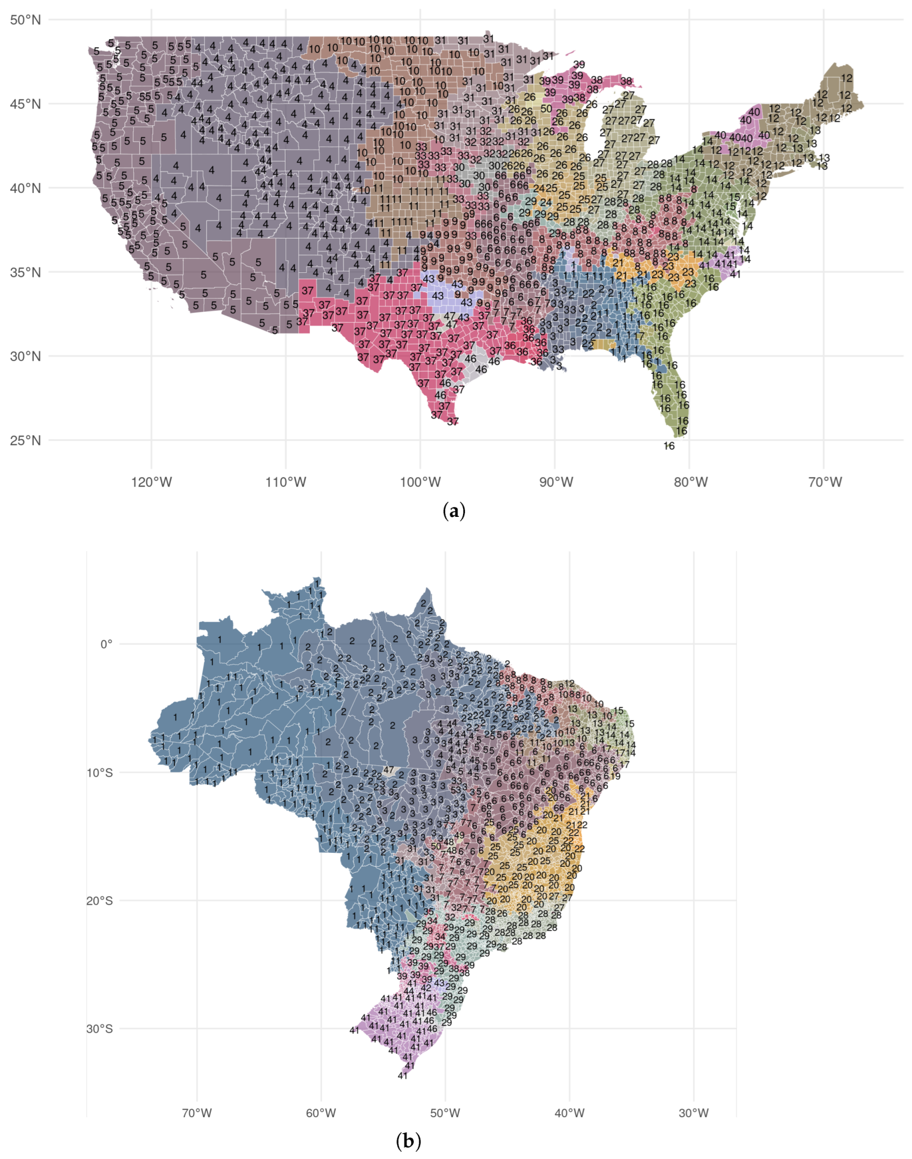
Our results so far illustrate that the structural relationship between nighttime lights and GDP varies with level of GDP, population density, and industrial composition. Since nightlights are used to proxy for economic activity at multiple subnational scales, we proceed to explore how the structural relationship between nightlights and GDP varies according to the size and number of subnational partitions in a country. Specifically, we test whether partitioning a country into subnational regions of different shapes and sizes affects how nightlights respond to increases in economic activity. We use disaggregated data from two countries, the United States and Brazil, that are at opposite ends of the income spectrum covered by our sample but are physically large and exhibit a varied pattern of regional economic specialization. Figure 4 shows an example of how we randomly partition the United States and Brazil into 50 administrative units.
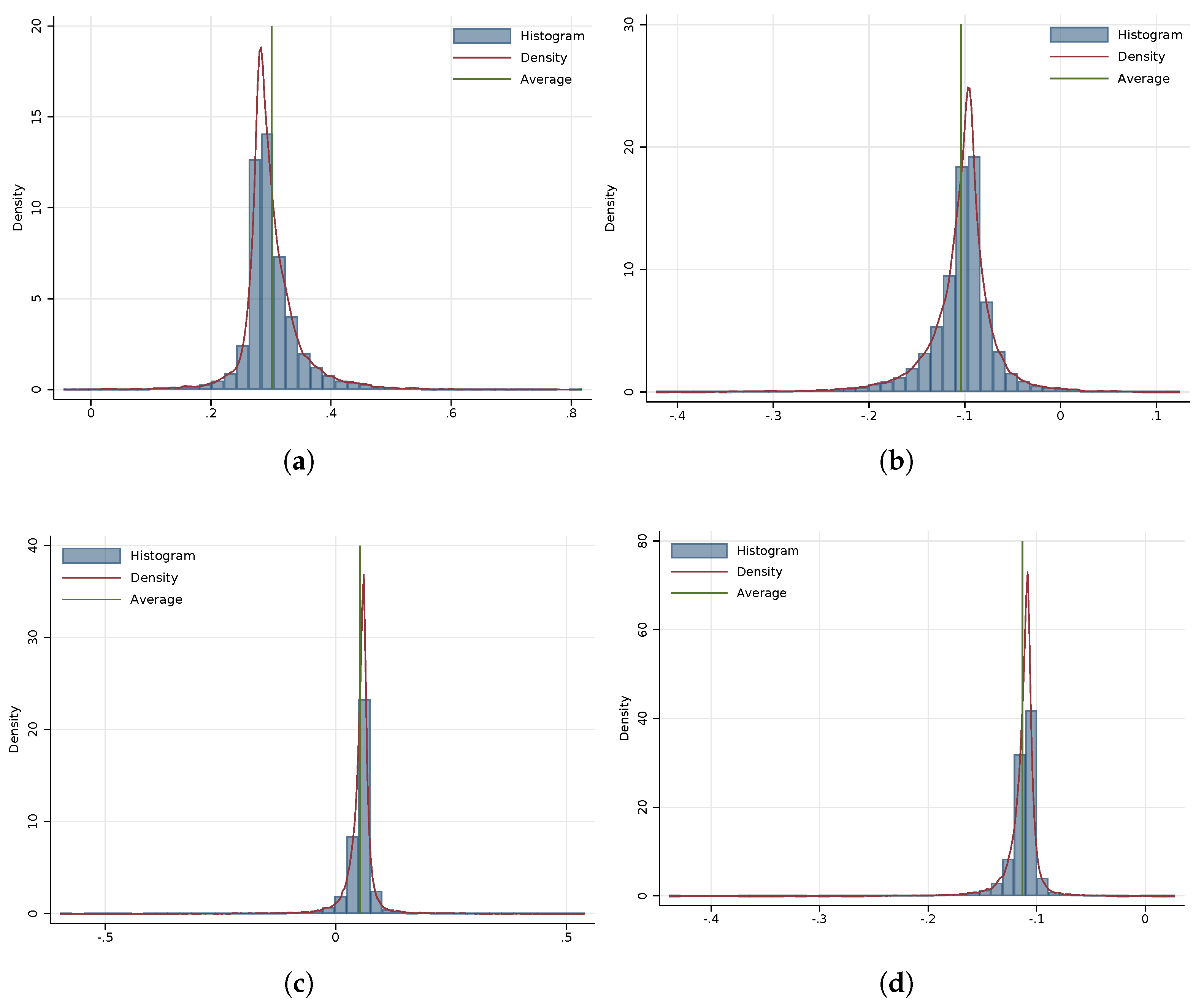
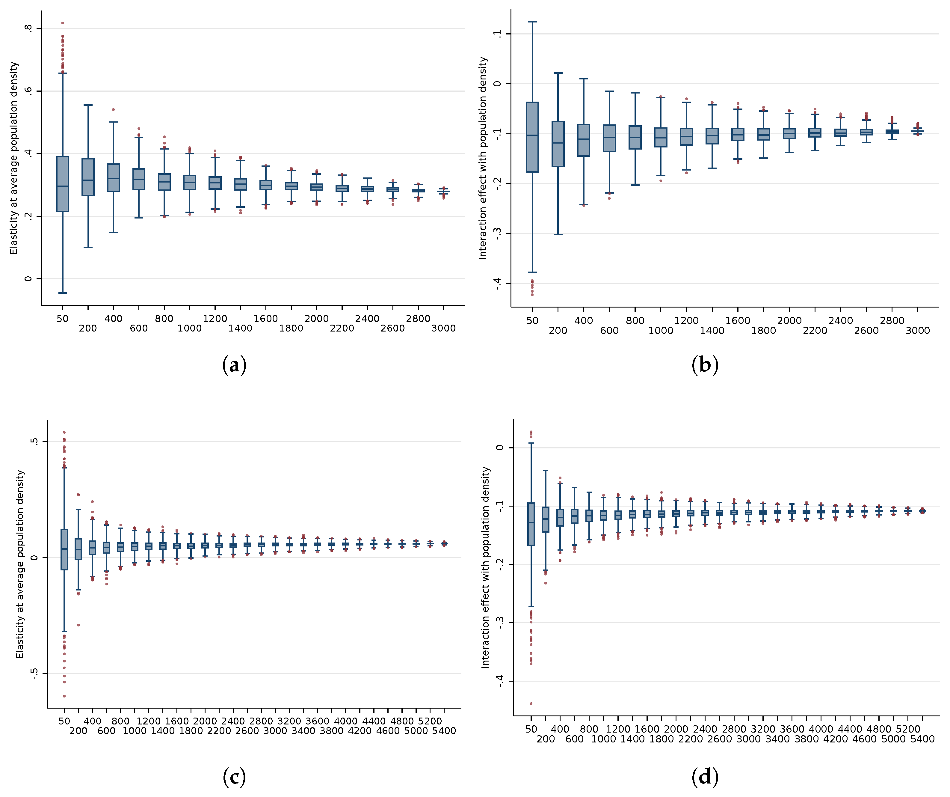
Figure 5 shows the distribution of estimates of Equation (2) for 16,200 simulations of partitions of the United States and 28,000 simulations of partitions of Brazil over which we aggregate nighttime lights, GDP, and population. For a given number of total units (ranging from 50–3000 for the United States and 50–5400 for Brazil), we simulate 1000 partitions in which the spatial aggregation of original units is based on a unique random starting seed in each iteration. We report results for the elasticity at the mean of population density ( β ^ ) and the interaction with population density ( γ ^ ) for the United States in Figure 5a,b and Brazil in Figure 5c,d. We observe that the overall average elasticity (at mean population density) is around 0.3 in the case of the US and 0.053 in the case of Brazil. Both of these values are close to the regression results presented in columns (1) and (5) of Table 3. For the US, almost every single estimated value using simulated partitions is larger than zero (99.97% of simulations) and does not contain zero in its 95% confidence interval (98.23%), while we estimate elasticities below zero only in 4.1% of the sampled partitions in the case of Brazil.
We find strong evidence of nonlinearity in nearly all simulated partitions. Figure 5b,d illustrate that the average of all simulated interaction coefficients is −0.104 for the US and −0.11 for Brazil (again close to Table 3). Less than 1% of the US estimates are positive and only 8.7% of the estimates include zero in their 95% confidence interval. Similarly, only 9 out of 28,000 simulations for Brazil yield a positive interaction coefficient and only about 1% cannot be distinguished from zero.
Figure 6 presents results conditional on the scale of spatial aggregation, that is, the number of administrative units. The random aggregation is simulated 1000 times for each total number of administrative units. We present the regression results as box-and-whisker plots (outliers outside the lower and upper adjacent values are indicated as red dots). Several features stand out. The elasticity at the mean of population density, shown in Figure 6a,c, is remarkably stable in both countries (a result which carries over to specifications without an interaction term, see Figure S4 in the Supplementary Materials). The conditional means fluctuate only moderately around the overall means documented above. While the mean is stable, the variance of the estimates increases markedly as the number of partitions become smaller and the average size of each unit increases. For relatively coarse levels of spatial aggregation, it is not difficult to find partitions at which we observe no relationship between nighttime lights and GDP over time. For example, at 50 artificial US “states”, large parts of the distribution of estimates cross zero and around 31% of the underlying coefficients contain zero in their 95% confidence interval, while almost every single draw for partitions of size 200 and more yields a coefficient for which we can reject the null hypothesis of zero. We observe a similar relationship in the data for Brazil, where around 89% of all estimated coefficients with partitions using 50 units have zero in their 95% confidence intervals but this figure drops to less than 10% at 2800 units and less than 1% at 3400 units.
The interaction effects in Figure 6b,d follow the same pattern of stable mean and increasing variance as the number of administrative units falls. A total of 59.7% of the partitions of the United States into 50 “states” yield estimates of the interaction term that cannot be distinguished from zero. This is particularly interesting in light of an estimate of −0.23 (with a standard error of 0.05) which we obtain when running our baseline regression on data aggregated to the actual US states. This value sits at the 10th percentile of the distribution of simulated results for partitions into 50 units and is more than 2.5 times larger than the average elasticity across all simulations. At 200 units, 37.4% contain zero in their 95% confidence interval, and at 800 units, this falls to 5.5%.
Taken together, these simulations demonstrate a robust association of lights with GDP and provide strong evidence of nonlinearity across different geographic scales. As aggregation reduces measurement errors, we take this as another indication that measurement errors are not the driving force behind this nonlinearity. Moreover, we show that it is easy to obtain insignificant results at high levels of aggregations, where the estimated elasticities depend on how larger regions align with the spatial structure of production and density.

4. Discussion

This article investigates whether the ability of the nighttime lights to pick up changes in GDP varies across subnational regions and their characteristics. We show theoretically that any variation in the structural light-output relationship spills over into estimating policy-relevant parameters in applied work using nightlights as an outcome. Measurement errors in both nightlights and economic activity complicate inference about this relationship. We develop a framework for assessing the implied, relative magnitude of measurement errors across subnational regions, and apply it to study heterogeneity in the light-output relationship in several countries with varying degrees of statistical capacity.
Our findings document significant variation in the relationship between economic activity and nightlights at the subnational level which cannot be explained by variation in measurement errors alone. Variation in the elasticity persists whether we estimate the elasticities by income group, economic sector, or specify interactions with population density. Moreover, the elasticities with respect to industry and service GDP declines as population density rises. The elasticity in the agricultural sector is much smaller (in the United States it is 20 times smaller than the industry elasticity and over 50 times smaller than the service sector elasticity) and less consistent across countries. Since services dominate the economies we study, pooling across sectors results in the nonlinearity by population density exhibited in the service sector. The evidence favoring these nonlinearities is most robust in countries with the highest statistical capacity. However, the relationship follows a similar, albeit noisier, pattern in the other countries in our sample.
The second contribution of our study is on the stability of the nonlinear nightlight-GDP relationship over different levels of spatial aggregation. We find that the nonlinear relationship is remarkably stable over many alternative administrative divisions of varying shapes and sizes. However, our estimates of the GDP elasticities are more stable under random partitions where the total number of regions is large (keeping their size small). At the same time, these smaller regions exhibit stronger nonlinearity since smaller units are more homogeneous in terms of population density, economic activity, and economic structure. At larger geographies, estimates are less stable, and there is a higher likelihood of drawing statistically insignificant estimates. This may help explain why other studies have failed to find significant relationships between nightlights and economic activity at some levels of aggregation [18]. It is also worth noting that the less precise estimates for Italy and Spain in our analysis are consistent with these two countries having the fewest number of regions.
We note that our findings provide a framework for reconciling other empirical research. Papers documenting the relationship between nightlights and economic activity at subnational scale have not found a consistent statistical relationship [18], and at smaller scales there is evidence for nonlinearity as well [2,7]. Our work helps scholars adjudicate between measurement error and structural nonlinearity in explaining observed nonlinearity in the NTL-GDP elasticity. We offer observable covariates such as population density, GDP density, and economic structure as predictors for the local NTL-GDP elasticity. We also show that larger subnational scales exhibit larger variation in the estimated elasticity.
Researchers using nightlights as a proxy for economic activity at small geographies, for example, to study the effects of conflict or measure economic inequality, need to be conscious of the variation we find in this paper. The income elasticity of nighttime lights may be considerably smaller in agricultural regions, regions with higher GDP, and regions with high population density. Changes in economic activity in such areas may result in small changes in nightlights that are, perhaps, not distinguishable from zero. As a result, a researcher may erroneously conclude that a policy or investment did not affect economic growth or inequality because the change in nightlights is insignificant (a null finding, of course, which includes a wide range of potential effects sizes in addition to zero). Moreover, even when the policy has an effect, additional analyses of treatment effect heterogeneity across regions may be driven solely by the heterogeneity of the light-output elasticity we document in this paper. The nonlinearity also implies that large changes in nightlights might occur in some contexts despite little change in economic activity.
In addition, our results suggest caution in taking estimates from other contexts to infer how changes in nightlights in a particular location translate into changes in GDP. The presence of a nonlinear relationship between nightlights and economic activity across subnational regions of different population densities, GDP levels, or economic structures means that researchers should consider whether taking an elasticity from the literature and applying it to a specific empirical context is appropriate. While such an elasticity might reflect the average relationship between nightlights and changes in economic activity over many subnational units, research focused on one or a small number of regions should rely on nightlights-GDP elasticities estimated from regions with similar characteristics and have some sense of the scale of measurement errors in their context. Moreover, research on agricultural, high GDP, or high population density settings may want to examine alternative proxies of economic activity and not make inferences only from nightlights.
While our work documents significant variation in the nightlights-income relationship, it has some fundamental limitations. First, we can only explore the relationship in countries with a sufficiently long panel of subnational GDP data. Our work considers a set of high-income and middle-income countries. It would have been ideal also to have data from low-income countries with robust statistical capacity that report subnational GDP because the research we are trying to inform is most often conducted in low-income settings where nightlights are one of the few available proxies for subnational GDP.
A second challenge is that the actual degree of measurement error in GDP at the subnational level is unknown. We use the elasticities across regions in countries with the highest statistical capacity—Germany and the United States—to conclude that the range is too wide to be explained by differences in measurement errors in GDP across regions. However, we can only infer this from the high statistical capacity of these countries and have no way to verify the true differences in measurement error in subnational GDP in any country. Moreover, we know very little about the scale of errors introduced by standard approaches to calculating (and usually scaling up) estimates of local GDP.
Finally, our study uses data on nighttime lights derived from a system with many known limitations. The main advantage of the dated DMSP-OLS system over the newer VIIRS data is that it allows us to study changes within regions over one or two decades, depending on the availability of GDP data. While we use a topcoding corrected version of this data to shut down one of the most likely sources of nonlinearity (which correlates with population density and GDP), we cannot entirely rule out that unfortunate features of the data generating process contribute to our findings.

Supplementary Materials

The following are available online at https://www.mdpi.com/article/10.3390/rs14051190/s1, Table S1: Income elasticity of topcoding corrected nighttime lights by population density. Figure S1: Estimates of relative measurement errors using topcoding corrected nighttime lights. Figure S2: Estimates of relative measurement errors using spatially correlated standard errors. Figure S3: Income elasticity of nighttime lights by log population density. Figure S4: Unconditional and conditional distribution of estimated elasticities across simulated partitions.

Author Contributions

R.B. and G.C.M. contributed equally to this work. All authors have read and agreed to the published version of the manuscript.

Funding

Richard Bluhm acknowledges financial support from the Alexander von Humboldt Foundation.

Data Availability Statement

Data and code are available at https://github.com/rbluhm/ntl_gdp (accessed on 22 February 2022).

Acknowledgments

We are grateful to two anonymous referees for providing thoughtful comments on the manuscript. Moreover, we have greatly benefited from discussions with Denis de Chrombrugghe on the measurement error framework and have received helpful comments from Prashant Bharadwaj and Teevrat Garg.

Conflicts of Interest

The authors declare no conflict of interest.

Appendix A. Analytic Background

This section derives in detail some of the equations used in the main text and provides the relevant background for our estimation strategy. All true (unobserved) quantities are denoted by ‘*’ and all observed variables are demeaned across units and time.

Appendix A.1. Estimating the Relative Sizes of the Measurement Errors Using Single Regressions

We first formalize the set up described in the main text. Both observed lights and GDP are observed with error:
y i t G = y i t G * + e i t G
y i t L = y i t L * + e i t L
In both equations, we assume that the the measurement errors are mean independent conditional on the values of the latent variable(s) and that there is no systematic bias in observed GDP or lights, such that E [ e i t G | y i t G * ] = E [ e i t L | y i t L * ] = 0 ,
Our structural model of interest is the constant elasticity model:
y i t L * = β y i t G * + ϵ i t
which is the relationship that is typically assumed in the related literature on measurement error in the light-output relationship and applied papers using a constant elasticity to translate their effects from changes in nighttime lights to changes in GDP. By the same logic of the assumptions made above, we require E [ e i t G ϵ i t | y i t G * ] = E [ e i t L ϵ i t | y i t G * ] = 0 .
In addition, a key assumption in our analysis is that the error term of GDP is not correlated with the error term in lights conditional on unobserved GDP, i.e., E [ e i t G e i t L | y i t G * ] = 0 . This assumption has been made in virtually all of the related literature on measurement errors in nighttime lights [2,3,26] but is not innocuous. While lights and GDP are quantified in very different ways (satellites vs. subnational accounting), their errors could still be correlated if, for example, topcoding in urban areas is (inversely) correlated with measurement errors in GDP. We use topcoding corrected data as a robustness check to rule out one potential source of such a correlation.
Substituting observed for unobserved quantities yields:
y i t L = β y i t G β e i t G + e i t L + ϵ i t
which we estimate as
y i t L = β y i t G + υ i t
where the composite error υ i t = ϵ i t β e i t G + e i t L does not satisfy the usual assumptions for consistency. Instead, it is well known that
β ^ p β σ y G * 2 ( σ y G * 2 + σ e G 2 ) = β λ
where σ y G * 2 is the variance true output and σ e G 2 the variance of the error in GDP. λ is known as the signal-to-noise ratio or the attenuation factor and, since 0 < λ < 1 , the bias is towards zero.
If we additionally assume that σ e G 2 behaves like a decreasing step-function in y G * , then we should also observe decreasing attenuation factors if we group the data by observed GDP. This assumption mirrors the good data country and bad data country samples used in [3] but conjectures that the variance of these errors varies across subnational units (and indicates statistical capacity). If the constant elasticity assumption is correct, then the true β is the same in different sub-samples of the data. Therefore, any ratio of coefficients where each coefficient is estimated separately on ordered samples of y G * , say high GDP and low GDP, identifies the relative size of the measurement errors:
β ^ h β ^ l p ( σ y G * 2 + σ e l G 2 ) ( σ y G * 2 + σ e h G 2 ) = λ h λ l = θ h .
In the main text we present estimates of these ratios and their standard errors for samples split along quartiles of average GDP, denoted as θ k = λ k / λ 1 for k = 1 , 2 , , 4 . In fact, the precise shape of the conditional heteroskedasticity in σ e G 2 ( y G * ) is not important. Any difference in the error variance across different subsamples of GDP will translate into differences in the estimated θ s. If we observe large and statistically significant deviations in these relative signal-to-noise ratios within countries with uniformly high statistical capacity, then we can interpret this as evidence against the constant elasticity model and in favor of variation in the structural elasticity.

Appendix A.2. Estimating the Coefficients in the Interacted Model

Suppose that instead of Equation (A3), the structural model of interest is
y i t L * = β y i t G * + γ y i t G * z i t + ϵ i t
where z i t is observed without error. In our application, z i t is population density in the initial year, which is considerably easier to observe than GDP. Of course, with γ = 0 we are back to the constant elasticity model assumed earlier.
Substituting observed for unobserved quantities results in
y i t L = β y i t G β e i t G + γ y i t G z i t γ e i t G z i t + e i t L + ϵ i t
which we estimate as
y i t L = β y i t G + γ y i t G z i t + υ i t
where the new composite error is υ i t = ϵ i t β e i t G γ e i t G z i t + e i t L .
In general, estimates of coefficients in models with more than one independent variable where one or more of these variables are measured with error are biased in an unknown direction. To see this, consider the formulae for the regression coefficients estimated on the basis of Equation (A10):
β ^ = v a r ( y i t G z i t ) c o v ( y i t L , y i t G ) c o v ( y i t G z i t , y i t G ) c o v ( y i t L , y i t G z i t ) v a r ( y i t G ) v a r ( y i t G z i t ) ( c o v ( y i t G z i t , y i t G ) ) 2
γ ^ = v a r ( y i t G ) c o v ( y i t L , y i t G z i t ) c o v ( y i t G , y i t G z i t ) c o v ( y i t L , y i t G ) v a r ( y i t G ) v a r ( y i t G z i t ) ( c o v ( y i t G , y i t G z i t ) ) 2
Typically, both β ^ and γ ^ depend on the true β , γ and several (co)variances, so that the direction of the bias is indeterminate.
In our case, however, it could be plausible that c o v ( y i t G , y i t G z i t ) = 0 , if we are willing to make the stronger assumptions that e i t G is independent of y i t G * , z and the structural error, and c o v ( ( y i t G * ) 2 z i t ) = 0 (which restricts the relationship between population density and unobserved GDP to be linear).
It is straightforward to see that under these conditions
β ^ p β σ y G * 2 ( σ y G * 2 + σ e G 2 )
which is the same as Equation (A6) and does not depend on the value of γ .
Similarly, we have
γ ^ p γ σ y G * z 2 ( σ y G * z 2 + σ e G 2 σ z 2 )
which is attenuated by the signal-to-noise ratio in the product of observed GDP with population density. In the constant elasticity case, γ = 0 , so γ ^ p 0 . Hence, any evidence rejecting the null of γ = 0 suggests that the constant elasticity model is incorrect (or that one or more of the assumptions made here is violated). Again, it is important to note that these results rely on substantially stronger assumptions than the single regression estimates presented above. We only view the resulting estimates as additional (and weaker) evidence on the whether the constant elasticity model is empirically supported.

References

  1. Elvidge, C.D.; Baugh, K.E.; Kihn, E.A.; Kroehl, H.W.; Davis, E.R.; Davis, C.W. Relation between satellite observed visible-near infrared emissions, population, economic activity and electric power consumption. Int. J. Remote Sens. 1997, 18, 1373–1379. [Google Scholar] [CrossRef]
  2. Chen, X.; Nordhaus, W.D. Using luminosity data as a proxy for economic statistics. Proc. Natl. Acad. Sci. USA 2011, 108, 8589–8594. [Google Scholar] [CrossRef] [PubMed] [Green Version]
  3. Henderson, J.V.; Storeygard, A.; Weil, D.N. Measuring economic growth from outer space. Am. Econ. Rev. 2012, 102, 994–1028. [Google Scholar] [CrossRef] [PubMed] [Green Version]
  4. Hodler, R.; Raschky, P.A. Regional Favoritism. Q. J. Econ. 2014, 129, 995–1033. [Google Scholar] [CrossRef]
  5. Storeygard, A. Farther on down the Road: Transport Costs, Trade and Urban Growth in Sub-Saharan Africa. Rev. Econ. Stud. 2016, 83, 1263–1295. [Google Scholar] [CrossRef] [Green Version]
  6. Jean, N.; Burke, M.; Xie, M.; Davis, W.M.; Lobell, D.B.; Ermon, S. Combining satellite imagery and machine learning to predict poverty. Science 2016, 353, 790–794. [Google Scholar] [CrossRef] [Green Version]
  7. Asher, S.; Lunt, T.; Matsuura, R.; Novosad, P. Development Research at High Geographic Resolution: An Analysis of Night-Lights, Firms, and Poverty in India Using the SHRUG Open Data Platform. World Bank Econ. Rev. 2021, 35, 845–871. [Google Scholar] [CrossRef]
  8. Kocornik-Mina, A.; McDermott, T.K.J.; Michaels, G.; Rauch, F. Flooded Cities. Am. Econ. J. Appl. Econ. 2020, 12, 35–66. [Google Scholar] [CrossRef]
  9. Lee, Y.S. International isolation and regional inequality: Evidence from sanctions on North Korea. J. Urban Econ. 2018, 103, 34–51. [Google Scholar] [CrossRef]
  10. Cook, C.J.; Shah, M. Aggregate Effects from Public Works: Evidence from India. Rev. Econ. Stat. 2020, 1–38. [Google Scholar] [CrossRef]
  11. Shenoy, A. Regional development through place-based policies: Evidence from a spatial discontinuity. J. Dev. Econ. 2018, 130, 173–189. [Google Scholar] [CrossRef]
  12. Weidmann, N.B.; Schutte, S. Using night light emissions for the prediction of local wealth. J. Peace Res. 2017, 54, 125–140. [Google Scholar] [CrossRef]
  13. Bruederle, A.; Hodler, R. Nighttime lights as a proxy for human development at the local level. PLoS ONE 2018, 13, 1–22. [Google Scholar] [CrossRef] [PubMed] [Green Version]
  14. Henderson, J.V.; Squires, T.; Storeygard, A.; Weil, D. The global distribution of economic activity: Nature, history, and the role of trade. Q. J. Econ. 2018, 133, 357–406. [Google Scholar] [CrossRef]
  15. Falchetta, G.; Pachauri, S.; Parkinson, S.; Byers, E. A high-resolution gridded dataset to assess electrification in sub-Saharan Africa. Sci. Data 2019, 6, 110. [Google Scholar] [CrossRef] [Green Version]
  16. Alder, S. Chinese Roads in India: The Effect of Transport Infrastructure on Economic Development. 2016. Available online: https://ssrn.com/abstract=2856050 (accessed on 1 February 2022).
  17. Hu, Y.; Yao, J. Illuminating economic growth. J. Econom. 2021. [Google Scholar] [CrossRef]
  18. Bickenbach, F.; Bode, E.; Nunnenkamp, P.; Söder, M. Night lights and regional GDP. Rev. World Econ. 2016, 152, 425–447. [Google Scholar] [CrossRef] [Green Version]
  19. Gibson, J.; Olivia, S.; Boe-Gibson, G.; Li, C. Which night lights data should we use in economics, and where? J. Dev. Econ. 2021, 149, 102602. [Google Scholar] [CrossRef]
  20. Tuttle, B.T.; Anderson, S.J.; Sutton, P.C.; Elvidge, C.D.; Baugh, K. It Used To Be Dark Here. Photogramm. Eng. Remote Sens. 2013, 79, 287–297. [Google Scholar] [CrossRef]
  21. Hsu, F.C.; Baugh, K.E.; Ghosh, T.; Zhizhin, M.; Elvidge, C.D. DMSP-OLS Radiance Calibrated Nighttime Lights Time Series with Intercalibration. Remote Sens. 2015, 7, 1855–1876. [Google Scholar] [CrossRef] [Green Version]
  22. Abrahams, A.; Oram, C.; Lozano-Gracia, N. Deblurring DMSP nighttime lights: A new method using Gaussian filters and frequencies of illumination. Remote Sens. Environ. 2018, 210, 242–258. [Google Scholar] [CrossRef]
  23. Bluhm, R.; Krause, M. Top Lights: Bright Cities and Their Contribution to Economic Development; SoDa Laboratories Working Paper Series 2020-08; SoDa Laboratories, Monash University: Melbourne, VIC, Australia, 2020. [Google Scholar]
  24. Devarajan, S. Africa’s Statistical Tragedy. Rev. Income Wealth 2013, 59, S9–S15. [Google Scholar] [CrossRef]
  25. Martinez, L.R. How Much Should We Trust the Dictator’s GDP Growth Estimates? Becker Friedman Institute for Economics Working Paper 2021-78; University of Chicago: Chicago, IL, USA, 2021. [Google Scholar]
  26. Pinkovskiy, M.; Sala-i Martin, X. Lights, Camera … Income! Illuminating the National Accounts-Household Surveys Debate. Q. J. Econ. 2016, 131, 579–631. [Google Scholar] [CrossRef]
  27. Heston, A.; Summers, R.; Aten, B. Appendix for a Space-Time System of National Account aka Penn World Table 5.6; Technical Report; Center for International Comparisons of Production, Income and Prices at the University of Pennsylvania: Philadelphia, PA, USA, 1994. [Google Scholar]
  28. Heston, A.; Summers, R.; Aten, B. Data Appendix for a Space-Time System of National Accounts: Penn World Table 6.1 (PWT 6.1); Technical Report; Center for International Comparisons of Production, Income and Prices at the University of Pennsylvania: Philadelphia, PA, USA, 2002. [Google Scholar]
  29. Gibson, J.; Boe-Gibson, G. Nighttime Lights and County-Level Economic Activity in the United States: 2001 to 2019. Remote Sens. 2021, 13, 2741. [Google Scholar] [CrossRef]
  30. Addison, D.M.; Stewart, B.P. Nighttime Lights Revisited: The Use of Nighttime Lights Data as a Proxy for Economic Variables; Policy Research Working Paper Series 7496; The World Bank: Washington, DC, USA, 2015. [Google Scholar]
  31. Briant, A.; Combes, P.P.; Lafourcade, M. Dots to boxes: Do the size and shape of spatial units jeopardize economic geography estimations? J. Urban Econ. 2010, 67, 287–302. [Google Scholar] [CrossRef] [Green Version]
  32. Openshaw, S.; Taylor, P. A million or so correlation coefficients: Three experiments on the modifiable area unit problem. In Statistical Applications in the Spatial Sciences; Wrigley, H., Ed.; Pion: London, UK, 1979; pp. 127–144. [Google Scholar]
  33. Fixler, D. Measurement error in the national accounts. In Measurement Error: Consequences, Applications and Solutions; Emerald Group Publishing Limited: Bingley, UK, 2009. [Google Scholar]
  34. Guci, L.; Mead, C.I.; Panek, S.D. A Research Agenda for Measuring GDP at the County Level; Bureau of Economic Analysis Working Paper; Bureau of Economic Analysis: Suitland, MD, USA, 2016.
  35. Aysheshim, K.; Hinson, J.R.; Panek, S.D. A Primer on Local Area Gross Domestic Product Methodology. Surv. Curr. Bus. 2020, 100, 1–13. [Google Scholar]
  36. European Commission. Eurostat Manuals and Guidelines: Manual on Regional Accounts Methods; European Commission: Brussels, Belgium, 2013.
  37. European Commission. Quality Report on National and Regional Accounts: 2016 Data; European Commission: Brussels, Belgium, 2018.
  38. European Commission. Quality Report on National and Regional Accounts: 2019 Data; European Commission: Brussels, Belgium, 2020.
  39. Instituto Brasileiro de Geografia e Estatística. Produto Interno Bruto dos Municípios, Ano de Referência 2010; Instituto Brasileiro de Geografia e Estatística: Rio de Janeiro, Brazil, 2016.
  40. National Bureau of Statistics of China. Announcement of the National Bureau of Statistics on the Final Verification of GDP in 2019. 2019. Available online: http://www.stats.gov.cn/english/PressRelease/202012/t20201231_1811928.html (accessed on 15 December 2020).
  41. Chen, W.; Chen, X.; Hsieh, C.T.; Song, Z. A Forensic Examination of China’s National Accounts. In Brookings Papers on Economic Activity; National Bureau of Economic Research: Cambridge, MA, USA, 2019. [Google Scholar]
  42. Määttä, I.; Lessmann, C. Human Lights. Remote Sens. 2019, 11, 2194. [Google Scholar] [CrossRef] [Green Version]
  43. Tuttle, B.T.; Anderson, S.; Elvidge, C.; Ghosh, T.; Baugh, K.; Sutton, P. Aladdin’s Magic Lamp: Active Target Calibration of the DMSP OLS. Remote Sens. 2014, 6, 12708–12722. [Google Scholar] [CrossRef] [Green Version]
  44. Ghosh, T.; Baugh, K.E.; Elvidge, C.D.; Zhizhin, M.; Poyda, A.; Hsu, F.C. Extending the DMSP Nighttime Lights Time Series beyond 2013. Remote Sens. 2021, 13, 5004. [Google Scholar] [CrossRef]
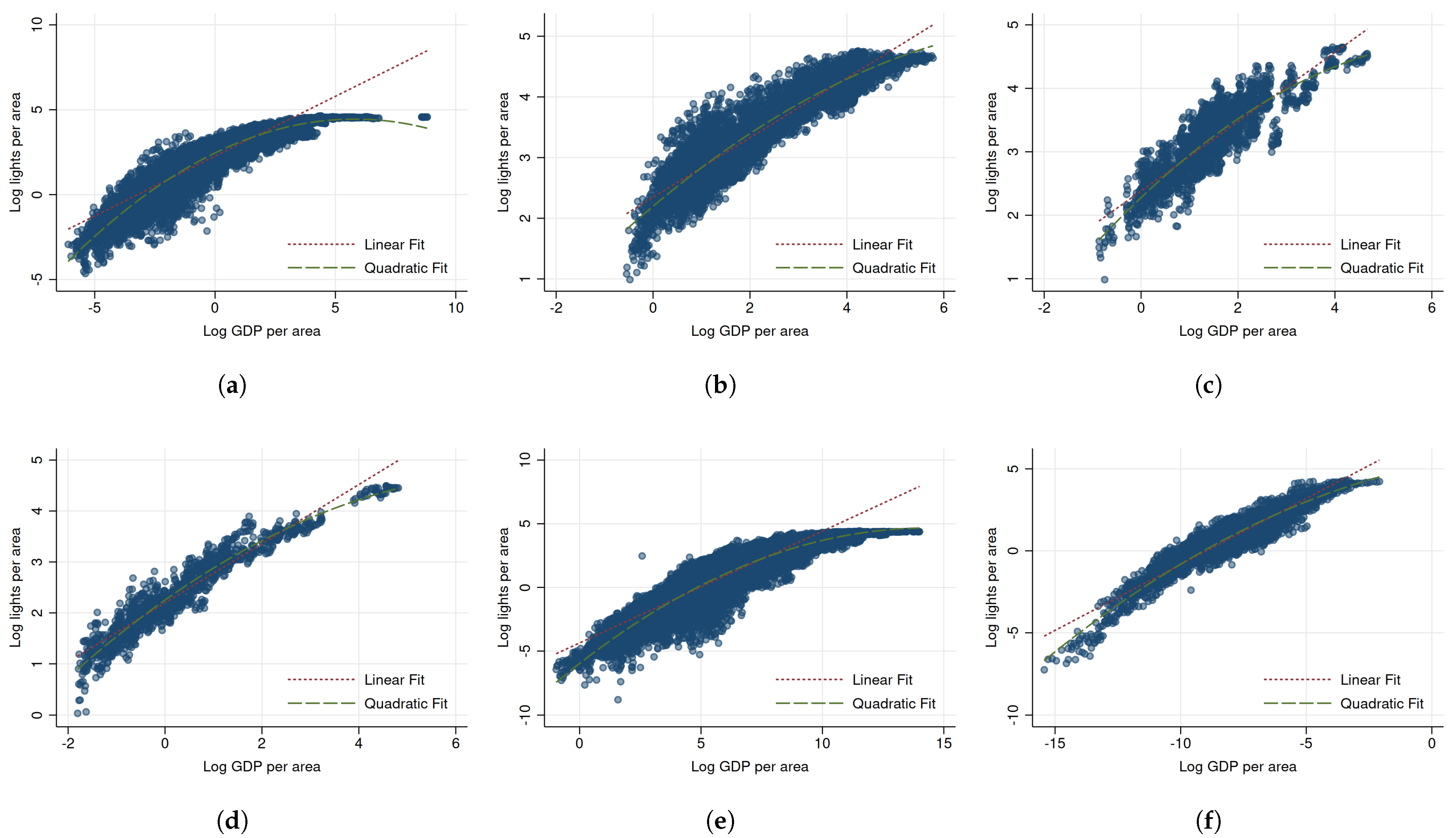
Figure 1. Raw correlation of nighttime lights with real GDP, in logarithms. (a) USA, (b) Germany, (c) Italy, (d) Spain, (e) Brazil, (f) China.
Remotesensing 14 01190 g001
Figure 2. Income elasticity of nightlights for samples split by quartiles of average GDP. (a) USA, (b) Germany, (c) Italy, (d) Spain, (e) Brazil, (f) China.
Remotesensing 14 01190 g002
Figure 3. Estimates of relative measurement errors for samples split by quartiles of average GDP. (a) USA, (b) Germany, (c) Italy, (d) Spain, (e) Brazil, (f) China.
Remotesensing 14 01190 g003
Figure 4. Examples of spatially contiguous random partitions. (a) USA: Partition 1 for 50 administrative units, (b) Brazil: Partition 1 for 50 administrative units.
Remotesensing 14 01190 g004
Figure 5. Unconditional distribution of estimates across partition simulations. (a) USA: Elasticity at average ( β ^ ), (b) USA: Interaction ( γ ^ ), (c) Brazil: Elasticity at average ( β ^ ), (d) Brazil: Interaction ( γ ^ ).
Remotesensing 14 01190 g005
Figure 6. Distribution of estimates across partition simulations, by number of units. (a) USA: Elasticity at average ( β ^ ), (b) USA: Interaction ( γ ^ ), (c) Brazil: Elasticity at average ( β ^ ), (d) Brazil: Interaction ( γ ^ ).
Remotesensing 14 01190 g006
Table 1. Sources of subnational GDP data.
CountryGeographyUnitsAvailabilityIndustrial Class.Source
USACounties30802001–2019NAICSBEA
GermanyDistricts4011992–2018NACE Rev. 2ADERCO
ItalyProvinces1101992–2018NACE Rev. 2ADERCO
SpainProvinces581992–2018NACE Rev. 2ADERCO
BrazilMunicipalities55692002–2018Primary to tertiaryIBGE
ChinaPrefectures3421999–2018n/aEIU
Notes: Data on counties in the United States are from the Bureau of Economic Analysis (BEA), which publishes data on real GDP by NAICS industry and population at the county level. We define all NAICS codes starting with 11 as agriculture, 21–33 as industry and 42–92 remaining codes as services. Data on German districts (Kreise), Italian provinces, and Spanish provinces (Provincias, islas, and Ceuta y Melilla) are from the Annual Regional Database of the European Commission’s Directorate General for Regional and Urban Policy (ADERCO). ADERCO publishes data on real GDP by NACE industry and population at the NUTS-3 (rev. 2016) level. We define all NACE codes starting with A as agriculture, B–E as industry and F as services. ADERCO includes historical estimates and projections for the most recent years. We only use data until 2018 which matches the availability of actual GDP figures reported by the relevant national offices. Data on Brazilian municipal GDP is from the Instituto Brasileiro de Geografia e Estatística (IBGE). GDP data exist for all 5570 municipalities, however 1 municipality had zero nightlights over the period (Marajá do Sena) and was dropped when taking logarithms. Data on Chinese prefecture-level GDP is available from the Economics Intelligence Unit (EIU) for 289 prefectures, and augmented with data for 53 more prefectures from Provincial Yearbooks or the CEIC Database.
Table 2. Distribution of nightlight density values across subnational regions.
Lights/AreaUSAGermanyItalySpainBrazilChina
00 (0%)0 (0%)0 (0%)0 (0%)367 (0.6%)0 (0%)
0–14179 (10.4%)0 (0%)0 (0%)0 (0%)25,551 (39.8%)889 (18.5%)
1–510,192 (25.5%)42 (0.5%)10 (0.41%)224 (17.3%)24,567 (36.8%)1873 (39.0%)
5–109354 (23.4%)346 (3.9%)125 (5.2%)393 (30.3%)7809 (11.7%)894 (18.6%)
10–208779 (21.9%)2888 (32.7%)759 (31.4%)323 (24.9%)4271 (6.4%)756 (15.7%)
20–505676 (14.2%)3040 (34.5%)1316 (54.4%)290 (22.3%)2249 (3.4%)335 (7.0%)
>501859 (4.6%)2506 (28.41%)210 (8.7%)68 (5.2%)952 (1.4%)55 (1.2%)
Notes: Lights/area refers to the sum of nighttime lights in a subnational region in a given year in the sample divided by the region’s area. Values refer to the number of region-years with the given level of nightlights per area, and the percentage in parentheses is the percentage of all observations from that country with that level of nightlight density.
Table 3. Income elasticity of nighttime lights by population density.
(1) USA(2) Germany(3) Italy(4) Spain(5) Brazil(6) China
Panel A: Real GDP density without interaction
GDP0.405 ***0.348 ***0.096−0.0920.100 ***0.292 ***
(0.043)(0.034)(0.081)(0.124)(0.015)(0.042)
Regions3080392110585569342
Observations40,03986242420127666,3984802
Panel B: Real GDP density interacted with Pop Dens
GDP0.278 ***0.291 ***0.072−0.0370.061 ***0.195 ***
(0.026)(0.025)(0.058)(0.126)(0.013)(0.037)
GDP × PopDens−0.094 ***−0.206 ***−0.275 ***−0.165 ***−0.108 ***−0.058 ***
(0.019)(0.015)(0.032)(0.031)(0.007)(0.009)
Regions3080392110585569342
Observations40,03986242420127666,3984802
Notes: Nightlights, GDP, and population density are all in logarithms. GDP refers to GDP density (GDP divided by region area) in constant prices. All regressions use the sum of lights divided by region area as the dependent variable. Panel A shows the constant elasticity model, while Panel B interacts GDP with the population density in the first year that region is included in the regression. All regressions include region and year fixed effects. Standard errors in parenthesis are clustered at the region level, and significance levels are denoted at conventional levels *** p < 0.01.
Table 4. Income elasticity of nighttime lights across economic sectors.
(1) USA(2) Germany(3) Italy(4) Spain(5) Brazil
Panel A: Agricultural GDP density
GDP0.008 ***−0.039 ***0.0060.069 **0.012 **
(0.002)(0.011)(0.020)(0.030)(0.005)
Regions2982392110585567
Observations31,42886242420127666,372
Panel B: Industrial GDP density
GDP0.146 ***0.157 ***0.073 *0.0140.058 ***
(0.017)(0.016)(0.037)(0.077)(0.006)
Regions2939392110585569
Observations30,68186242420127666,363
Panel C: Service sector GDP density
GDP0.458 ***0.315 ***0.034−0.0850.140 ***
(0.065)(0.035)(0.078)(0.121)(0.015)
Regions2872392110585569
Observations27,60886242420127666,396
Notes: Nightlights and GDP are in logarithms. All regressions use the sum of lights divided by region area as the dependent variable. Panel A uses GDP in the agricultural sector (multiplying regional GDP by the share of agriculture in GDP) in constant prices, divided by region area to produce a GDP density. Panel B uses real GDP density in the industrial and construction sectors, and Panel C uses real GDP density in the service sector. All regressions include region and year fixed effects. For all regressions, standard errors in parenthesis are clustered at the region level. Significance levels denoted at conventional levels *** p < 0.01, ** p < 0.05, * p < 0.1.
Table 5. Income elasticity of nighttime lights by population density and by economic sector.
(1) USA(2) Germany(3) Italy(4) Spain(5) Brazil
Panel A: Agricultural GDP density
GDP0.006 ***−0.0110.0010.0280.011 **
(0.002)(0.012)(0.022)(0.036)(0.005)
GDP × PopDens−0.005 ***−0.035 ***0.054 **0.033 **−0.007 *
(0.001)(0.009)(0.023)(0.013)(0.004)
Regions2982392110585567
Observations31,42886242420127666,372
Panel B: Industrial GDP density
Real GDP0.113 ***0.159 ***0.088 **0.0640.045 ***
(0.012)(0.016)(0.042)(0.072)(0.005)
GDP × PopDens−0.045 ***−0.046 ***0.043−0.084 ***−0.033 ***
(0.012)(0.013)(0.042)(0.019)(0.004)
Regions2939392110585569
Observations30,68186242420127666,363
Panel C: Service sector GDP density
Real GDP0.232 ***0.237 ***0.036−0.0380.105 ***
(0.032)(0.031)(0.047)(0.122)(0.013)
GDP × PopDens−0.115 ***−0.197 ***−0.231 ***−0.167 ***−0.118 ***
(0.029)(0.013)(0.022)(0.026)(0.007)
Regions2872392110585569
Observations27,60886242420127666,396
Notes: Nightlights, GDP and population density are all in logarithms. All regressions use the sum of lights divided by region area as the dependent variable. Panel A uses GDP in the agricultural sector (multiplying regional GDP by the share of agricultural share in GDP), divided by region area to produce a GDP density. Panel B uses real GDP density in the industrial and construction sectors, and Panel C uses real GDP density in the service sector. PopDens refers to the population density in the first year that region is included in the regression. All regressions include region and year fixed effects. For all regressions, standard errors in parenthesis are clustered at the region level. Significance levels denoted at conventional levels *** p < 0.01, ** p < 0.05, * p < 0.1.
Publisher’s Note: MDPI stays neutral with regard to jurisdictional claims in published maps and institutional affiliations.