Article

Using Multi-Source Nighttime Lights Data to Proxy for County-Level Economic Activity in China from 2012 to 2019

Department of Economics, University of Waikato, Private Bag 3105, Hamilton 3240, New Zealand
*
Author to whom correspondence should be addressed.
Remote Sens. 2022, 14(5), 1282; https://doi.org/10.3390/rs14051282
Submission received: 22 January 2022 / Revised: 23 February 2022 / Accepted: 1 March 2022 / Published: 5 March 2022
(This article belongs to the Special Issue Applications of AI and Remote Sensing in Urban Systems)

Abstract

:
The use of nighttime lights (NTL) data to proxy for local economic activity is well established in remote sensing and other disciplines. Validation studies comparing NTL data with traditional economic indicators, such as Gross Domestic Product (GDP), underpin this usage in applied studies. Yet the most widely cited validation studies do not use the latest NTL data products, may not distinguish between time-series and cross-sectional uses of NTL data, and usually are for aggregated units, such as nation-states or the first sub-national level, yet applied studies increasingly focus on smaller and lower-level spatial units. To provide more updated and disaggregated validation results, this study examines relationships between GDP and NTL data for 2657 county-level units in China, observed each year from 2012 to 2019. The NTL data used were from three sources: the Defense Meteorological Satellite Program (DMSP), whose time series was recently extended to 2019; and two sets of Visible Infrared Imaging Radiometer Suite (VIIRS) data products. The first set of VIIRS products is the recently released version 2 (V.2 VNL) annual composites, and the second is the NASA Black Marble annual composites. Contrasts were made between cross-sectional predictions for GDP differences between areas and time-series predictions of economic activity changes over time, and also considered different levels of spatial aggregation.

1. Introduction

The use of nighttime lights (NTL) data to proxy for economic activity is well-established in remote sensing and other disciplines [1,2,3,4,5,6,7,8,9,10]. This proxy enables research when traditional economic activity data, such as Gross Domestic Product (GDP), are either absent or are not trusted because of concerns about either measurement error or manipulation [11,12,13]. Potential advantages of NTL-based economic activity estimates are their timeliness, lower cost, comparability between countries irrespective of statistical capacity, and availability for spatial units below the level at which GDP data are reported.
Early studies focused on cross-sectional comparisons of nations and sub-national regions, but more recent studies use NTL data to track changes in economic activity. These fluctuations may be due to natural disasters, such as earthquakes, floods, hurricanes, and tsunami [14,15,16,17,18]; public health crises, such as COVID-19 [19,20,21]; or to various economic policies [22,23]. This use of NTL as a proxy for changes in local economic activity, plus ongoing cross-sectional use as a proxy for variation in economic performance [24], raises the question of how good are the NTL data for studying differences in economic activity between areas and for studying the temporal changes in economic activity within areas.
Extant evidence is that changes in nighttime lights data poorly predict temporal changes in economic variables despite NTL data being good cross-sectional predictors of differences in economic activity across space within these same studies [25,26]. These studies with negative findings on the performance of NTL data as a proxy for temporal changes in economic activity use Defense Meteorological Satellite Program (DMSP) data and either contrast the shares of variation in economic indicators explained cross-sectionally and temporally, or else contrast cross-sectional and time-series elasticities of economic variables with respect to NTL data. Another approach with DMSP data estimates optimal weights for mixtures of NTL data and conventional economic statistics to best proxy for the true but unknown levels of, and changes in, economic activity [4,27]. Given that the DMSP data were not originally gathered for research purposes, in contrast to newer research-based products from the Visible Infrared Imaging Radiometer Suite (VIIRS) onboard the Suomi-NPP satellite [28], a relevant question is whether poor performance of NTL data for studying temporal changes in economic activity is a feature just of DMSP data or also applies to VIIRS data.
Some evidence suggests that poor predictive performance for time-series changes in local GDP also extends to the newer VIIRS data. In the United States, the share of variation in annual changes in GDP predicted by annual changes in VIIRS data is just 2% at the metropolitan level [29] or 12% at the county-level [30], yet VIIRS data predict almost 90% of the cross-sectional variation in GDP. However, the United States is a mature economy that has been highly urbanized for many decades, and so the scope for nighttime lights to change in response to economic fluctuations may be relatively low. In contrast, countries where NTL data are most useful for research tend to be undergoing rapid urbanization and electrification as part of their development process and so may have stronger relationships between changes in local economic activity and changes in NTL data. Therefore, this study examines relationships between GDP and NTL data for 2657 county-level units in China, observed each year from 2012 to 2019. The NTL data used are from three sources: DMSP stable lights annual composites [31], whose time-series was recently extended to 2019; and two sets of VIIRS data products—newly released version 2 (V.2 VNL) annual composites [32], and the NASA Black Marble annual composites [33]. Contrasts are made between cross-sectional predictions for GDP differences between counties and time-series predictions of economic activity changes over time. Recent monthly relationships between China’s electricity consumption and the various NTL data products are also examined.
In order for the results to provide informative comparisons with prior literature, the estimation framework is deliberately based on that from a study on the United States [30], where panel data provide “within” and “between” elasticities of GDP with respect to NTL data that correspond to the time-series and cross-sectional uses of these data. This framework is also based on the approach used in the most widely cited study of the relationship between GDP and NTL data [5]. If a different estimation framework was used, it would be difficult to draw broader lessons because differences in results between studies may be due to the different methods. This matters particularly for validation studies, such as the current study, which provide elasticity estimates for applied studies to use when converting estimated effects on NTL data into equivalent effects on economic activity; if the validation studies use heterogeneous methods, it reduces the scope for this transferability.

2. Materials and Methods

2.1. Related Literature on NTL Validation Studies

Validation studies set out to estimate the nature of relationships between NTL data and benchmark traditional economic activity data. These studies can provide support for use of NTL data as a proxy in times and places where traditional economic activity data, such as GDP, are unavailable. Validation studies may be stand-alone [4,5,29,30,34,35], or else may be part of a broader study where the validation exercise aims to justify the use of NTL data in the main analysis [36,37]. The most widely cited study (with 2120 Google Scholar citations as of January 2022) used national-level DMSP data and GDP data for 188 countries from 1992 to 2008 to estimate an elasticity of 0.3 for temporal changes in GDP with respect to changes in the NTL data [5]. A similar highly cited study (with 730 Google Scholar citations) used DMSP data for 1500 regions (mostly at the first sub-national level) from 82 countries from 1992 to 2009 and estimated that the elasticity for temporal changes in GDP with respect to temporal changes in DMSP data was 0.4 [36].
Although widely cited, these studies may be less informative in the present era due to two factors: much of the literature has moved on from DMSP and now uses VIIRS data, and applied studies using NTL data to proxy for economic activity increasingly use spatial units that are lower in the sub-national administrative hierarchy, such as districts (or other second-level units), counties (or other similar third-level units), and even individual pixels. An important interpretation issue is posed by the fact that the widely cited validation studies are typically based on DMSP data for spatially aggregated units. Meanwhile, the applied studies that cite the validation studies and that may use elasticity estimates reported by the validation studies in order to convert effects on NTL data into economic activity terms are increasingly based on lower level spatial units and increasingly are using VIIRS data. The elasticity estimates from DMSP data may not be applicable to results estimated with VIIRS data, and, likewise, it may be incorrect to transfer elasticity estimates from spatially aggregated validation studies into spatially disaggregated applied studies. A problem with such a transfer of the elasticity estimates is that flaws in DMSP data, such as geo-location errors and blurring [38,39], seem to make predictive performance for GDP worse when using lower-level spatial units than when using aggregated spatial units [35].
The validation studies using VIIRS data to examine time-series and cross-sectional predictions of GDP have concentrated on the United States. Almost 90% of cross-sectional variation in metropolitan-level GDP was predicted by variation in the sum of VIIRS radiances, but just 2% of annual changes in GDP were predicted by the annual changes in the NTL data, albeit with only a three-year time series [29]. A longer time-series from 2014 to 2019, estimated at the county-level, found 12% of temporal variation in GDP predicted by temporal variation in the sum of VIIRS nighttime lights, using data products that were masked to remove outliers, while the NTL data were able to predict 86% of the cross-sectional variation in economic activity [30]. In terms of elasticities of county-level GDP with respect to NTL data, the cross-sectional estimates averaged 1.0 while time-series elasticities for annual changes were just one-tenth as large, averaging 0.1. Thus, not only are relationships between temporal changes in nighttime lights and changes in economic activity far weaker than are the cross-sectional relationships in the levels, the elasticities found with VIIRS data are far lower than the values of 0.3 or 0.4 reported in widely cited validation studies using DMSP data for the national or first sub-national level [5,36].
This difference between the elasticities estimated from temporal changes and those that are estimated from cross-sectional differences affects the interpretation of several recent applied studies. Applied studies estimate the effects on nighttime lights of a particular shock or intervention, such as flooding [15], tsunami [17], or social transfers [40]. In order to convert these effects into equivalent effects on economic activity, they use estimates from the literature on the elasticity of GDP with respect to NTL data (because these applied studies lack GDP data for their own setting). While a popular choice for the elasticity used is 0.3, based on annual changes in national GDP and national DMSP lights [5], in some cases, they use much higher elasticities and so get larger calculated effects on economic activity of the shock or intervention that they study. Some of these larger elasticity estimates are from cross-sectional studies when it is the far smaller time-series elasticities that are appropriate inputs into their calculation [26].
While many studies have linked NTL data to sub-national GDP data for China, these are typically either correlational [7] or involve regressions in a framework that does not allow the time-series elasticities for temporal changes to be estimated separately from the cross-sectional elasticities for differences across space with, instead, some mixture of the two types of parameters estimated [41]. Two studies using the framework that allows the time-series elasticities to be estimated separately, with DMSP data at the prefectural level (the second sub-national level), find elasticities of 0.25 for changes in GDP with respect to changes in DMSP stable lights over 1992–2005 [37], and an elasticity of 0.30 (for urban parts of prefectures and 0.19 for rural parts), over 2000–12 [42]. Thus, the prior results for China provide elasticities that are similar to the elasticities from the highly cited worldwide studies [5,36], and these serve as a point of comparison for the new results reported below.

2.2. Data

We use four types of data to test the relationships between China’s nighttime lights and GDP. The first is annual information on the total GDP (in billions of Chinese Yuan, CNY) for each county-level unit from 2012 to 2019, which is obtained from three types of publications: the annual editions of the China Statistical Yearbook (county-level) (also named in Chinese as Zhongguo Xianyu Tongji Nianjian), annual editions of the China City Statistical Yearbook (also known in Chinese as Zhongguo Chengshi Tongji Nianjian), and annual editions of the Statistical Yearbook for each city (for example, the Beijing Statistical Yearbook) [43,44,45]. Each edition reports on GDP the previous year, so we use the 2013 to 2020 editions to obtain 2012 to 2019 GDP data. As of 2020, the county-level units in China were comprised of the following types: 965 municipal districts (that are highly urbanized), 387 county-level cities, 1323 counties, 117 autonomous counties, 49 banners, 3 autonomous banners, 1 special zone, and 1 forestry zone, and it is this diversity of types of units that necessitates using several different types of statistical yearbooks.
From a total of 2846 county-level units under the current administrative geography, we were able to create a balanced panel of GDP data for 2657 units (about 94% of the total) in each year from 2012 to 2019. The provinces with the largest number of spatial units for which we were not able to obtain the county-level GDP data were Tibet, Heilongjiang, and Xinjiang (Figure 1). Usually, the other occurrences of unavailable county-level GDP data were at most one or two per province, although for Qinghai, the two units with missing data are physically large and so occupy a prominent position on the map. Given the data that we have, our results can be thought of as representing almost 95% of China.
The second data source was annual composites from Defense Meteorological Satellite Program (DMSP) satellites F15 and F18. The stable lights product provides 6-bit digital numbers (DN) ranging from 0 to 63 for each 30 arc-second output pixel. Ephemeral lights, such as from fires and flaring, are removed, and processing excludes (at the pixel level) images for nights affected by clouds, moonlight, sunlight, and other glare. The usual stable lights product time-series ended in 2013 [31], but that has now been extended with images from F15 for 2014–19 [46]. The time of night that lighting is observed differs between the extended time-series using F15 (ca. 3.30 a.m.) and the original series with F18 (ca. 8.30 p.m.), and there may also be sensor differences, as F15 has been in orbit for longer, so more depreciation may have affected the equipment. The estimation framework controls for year-by-year differences using time fixed effects (separate intercepts for each year). Given that there is no overlap in time between the F15 and F18 time series, with one ending in 2013 and the other starting in 2014, these fixed effects will adjust for satellite-specific measurement differences (and in this way provide a form of inter-calibration, especially because all variables in the regressions outlined below are in logarithms). Moreover, if the 2014 year fixed effect is interacted with either the DN value from DMSP or the radiance values from the other NTL data sources, there is no statistically significant interaction effect, which supports the sole use of the year fixed effect as a straightforward intercept shifter to synthesize the values from the two time-series.
The third data source was version 2 VIIRS nighttime lights (V.2 VNL) annual composites [32]. The V.2 VNL are produced from monthly cloud-free radiance averages, with initial filtering to remove extraneous features, such as fires and aurora, before the resulting rough annual composites are subjected to outlier removal procedures. To isolate lit grid cells from background, a data range threshold is based on a multiyear maximum median and a multiyear percent cloud-cover grid. In contrast, version 1 annual composites [47] used year-specific thresholds, which are less suitable for change detection (given that different average radiance values between years could be due to on-the-ground changes or to differences in the thresholds). The data are in units of nano Watts per square centimeter per steradian (nW/cm2/sr) reported on a 15 arc-second output grid. We mainly use the average masked data product, which had the highest predictive power for GDP amongst all of the V.2 VNL data products in a study of the United States [30].
The fourth data source was NASA Black Marble VIIRS annual composites [33]. These use a bi-directional reflectance distributional function (BRDF) to remove the effects of extraneous artifacts, and processing also removes cloud-contaminated pixels. The data products are corrected for atmospheric, terrain, vegetation, snow, lunar, and stray light effects on VIIRS Day/Night Band (DNB) radiances and are calibrated across time and validated against ground measurements. The data are in units of nano Watts per square centimeter per steradian (nW/cm2/sr) reported with 16-bit precision on a 15 arc-second output grid. We use the all-angle composites, which are built from the greatest number of nights per year, compared to either the near-nadir (view zenith angle of 0–20 degrees) composites or the off-nadir (view zenith angle of 40–60 degrees) composites.
For the three NTL data products described above—DMSP DN values, V.2 VNL masked average radiances, and radiance values from the various Black Marble products—the sum of lights in each cross-sectional unit (typically a county-level unit) in each year is used as the measure of luminosity. This corresponds to annual GDP; that is, the sum of all measured economic activity within the cross-sectional unit in the particular year.
Even though we use annual composites, of either DN values for DMSP or radiances for V.2 VNL and for Black Marble, the available files also provide a tally, for each output grid cell, of the number of nights per year that were used to form the annual composite. For example, this tally of the number of nights is available in the cf_cvg.tif file associated with the DMSP stable lights composite. These tallies of the number of nights provide an indication of the variation in the completeness of temporal coverage for each of the NTL data products in each grid cell in each year and also provide a diagnostic tool for helping with the choice of particular radiance composite data products to use.
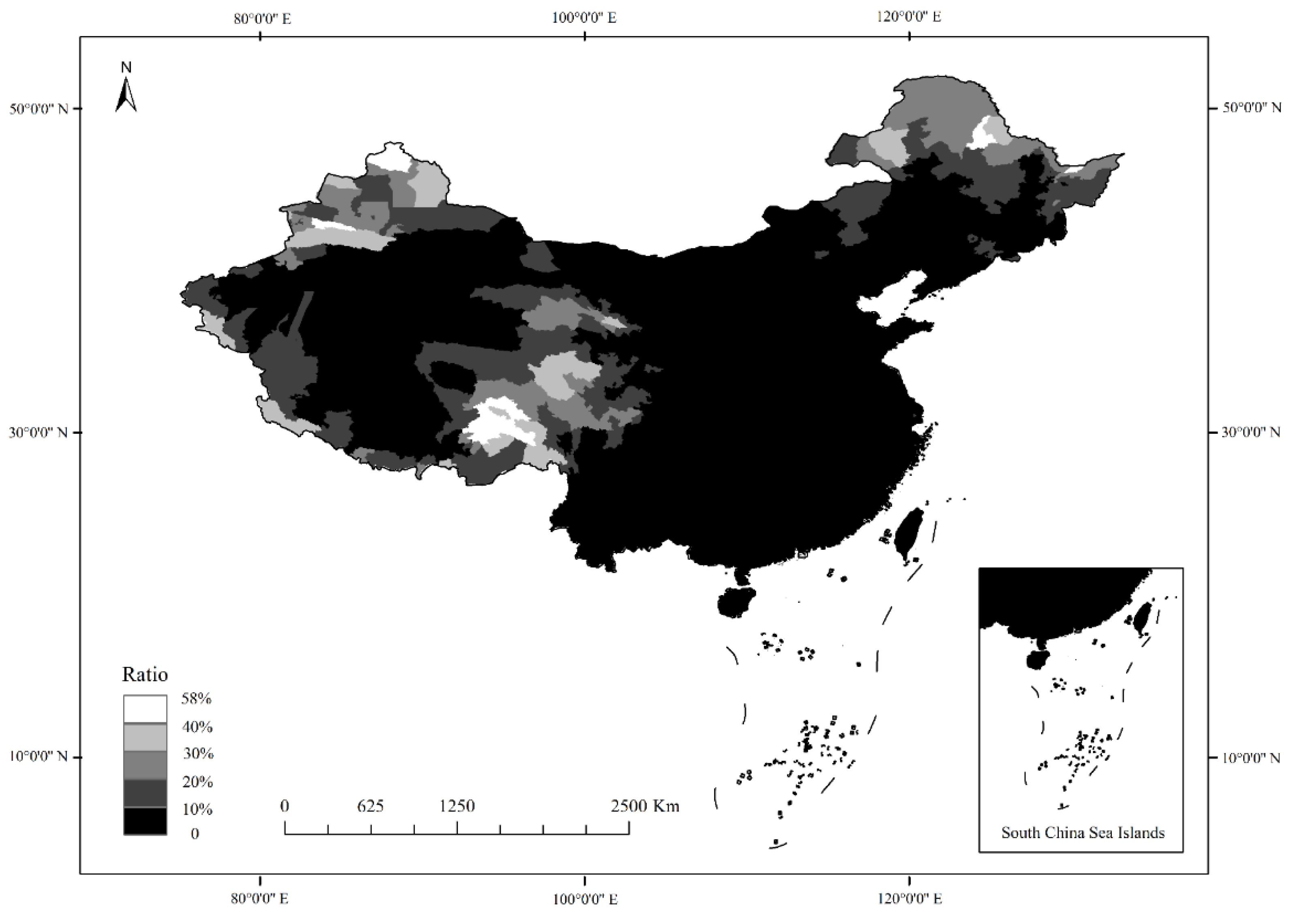
A feature of the Black Marble annual composites is the separation into snow-free and snow-covered periods. For parts of northern Xinjiang, northern Heilongjiang, and from the Tibetan plateau through Qinghai and Gansu, one-fifth or more of the nights in the year available for forming annual composites are snow-covered (Figure 2). While only using the all-angle snow-free composite in southern and eastern China should not distort the analysis of annual data, given that almost no-nights are snow-covered in these areas, for other parts of China, the omission of snow-covered nights may matter. Overall for China, ten percent of nights each year that meet quality control standards for inclusion in annual composites are snow-covered. Therefore, in addition to using existing snow-free annual composites, we created a weighted average of the snow-free and snow-covered composites. The weights are the number of snow-free days and of snow-covered days per year for each pixel. The weighted average should capture variation across the entire year in the same manner that annual GDP aggregates over all of the seasons.
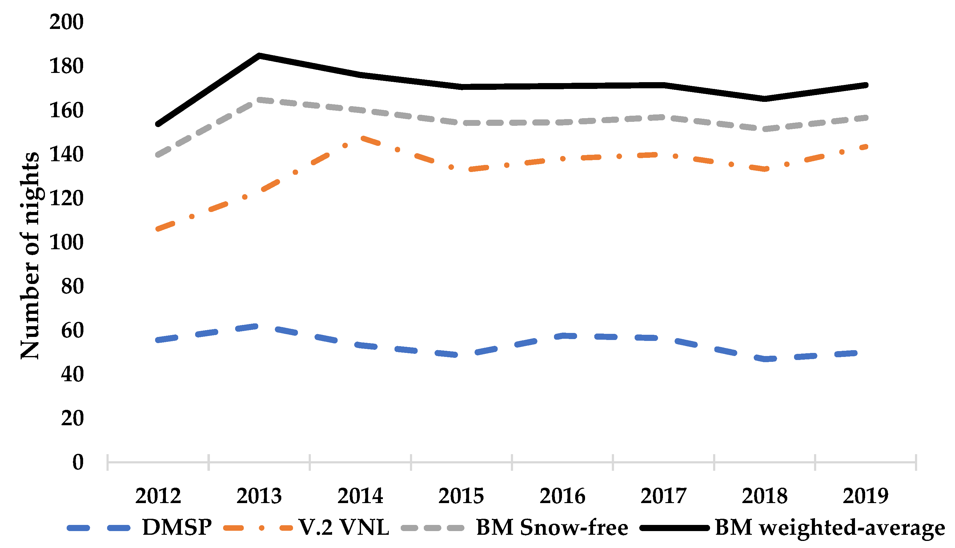
The average number of nights per year (averaged across all pixels in China) that are used to form the annual composites varies from around 50 nights per year for the DMSP stable lights composites to about 170 nights per year for the Black Marble composites that use weighted averages of the snow-free and snow-covered nights (Figure 3). On average, using the weighted average of snow-free and snow-covered composites gives about ten percent more nights per year than just relying on the snow-free composite, although as seen in Figure 2, the China-wide average disguises a lot of regional heterogeneity. Even though the V.2 VNL composites and the Black Marble composites rely on the same VIIRS source data, the different processing approaches result in 20–50% more nights being used in the formation of the Black Marble composites, particularly in the early years of the study period. All else the same, if more nights of the year are used to form an annual composite for an NTL data product, it should provide a more precise estimate of true luminosity. Moreover, to the extent that GDP covers economic activity over the entire course of the year, there may be a closer relationship between NTL data and GDP data for NTL products that are based on more nights of the year.
The attributes of the three NTL data sources are summarized in Table 1. The top part of the table covers satellite and sensor attributes, which are the same for both V.2 VNL and Black Marble (so only one column is used), and the bottom part of the table covers the attributes of the various data products.

2.3. Estimation Framework

Our estimation framework relies on the following equation (where ln is logarithm):
ln ( G D P ) i t = α + β ln ( s u m   o f   l i g h t s ) i t + μ i + φ t + ε i t
where the i indexes cross-sectional units; the t indexes years; the μ i are fixed effects for each cross-sectional unit; the φ t are fixed effects for each year; and ε i t is the disturbance term. The parameter of greatest interest is β , the elasticity of GDP with respect to nighttime lights. The elasticity is a unit-free measure showing by what percentage the left-hand side variable changes for each percentage change in the right-hand side variable. The fixed effects capture the influence of unobserved time-invariant features of each cross-sectional unit and the influence of spatially-invariant features of each time period.
This framework applied to panel data allows two different types of elasticities to be estimated. If Equation (1) is averaged over time, we get:
ln ( G D P ) ¯ i = β B ln ( s u m   o f   l i g h t s ) ¯ i + μ i + ε ¯ i
where time-averaged values of (log) GDP and NTL are used in a cross-sectional regression estimated with Ordinary Least Squares, to yield β B , which is known as the between estimator [48]. The elasticity in Equation (2) represents the effects of long-run differences between the cross-sectional units [49]. The second type of elasticity, β W , is known as the within estimator, where the variation over time within each cross-sectional unit provides the basis for estimating:
ln ( G D P ) i t ln ( G D P ) ¯ i = β W [ ln ( s u m   o f   l i g h t s ) i t ln ( s u m   o f   l i g h t s ) ¯ i ] + ε i t ε ¯ i  
Equation (3) is based on subtracting Equation (2) from Equation (1), and in doing so, it removes the effect of the unobservable fixed effects. Note that Equation (3) provides equivalent estimates to what would be obtained by estimating Equation (1) with separate intercepts for every cross-sectional unit. The between estimator β B , enables examination of the cross-sectional GDP differences between areas, while the within estimator β W , allows examination of the annual time-series fluctuations in GDP within areas.
If Equation (1) is estimated without fixed effects, or equivalently if time-demeaned data are not used, the resulting estimator for β will be a weighted average of the between estimator and the within estimator [50]. In other words, the resulting parameter will not identify either the long-run cross-sectional relationship, nor the effect of temporal changes. Thus, estimating Equation (1) without fixed effects will upwardly bias the estimator of β if it is being interpreted as a measure of the relationship between temporal changes in economic activity and temporal changes in NTL data. This upward bias is because the μ i should positively correlate with both GDP and nighttime lights due to the fact that topography and other environmental factors that limit urbanization and electrification in particular places (and therefore limit the amount of nighttime light emitted) would also be expected to limit the value of GDP produced in such places.
This upward bias affects the validity of using NTL data to estimate impacts on the local economic activity of policy interventions or shocks (more generally, of ‘treatments’). The product of two relationships: ( G D P / l i g h t s ) · ( l i g h t s / t r e a t m e n t ) is the basis of this approach to using NTL data for impact evaluation. In the settings of interest, typically, the G D P / l i g h t s relationship is not estimated because there are no GDP data (as any available and trustworthy GDP data would already be used for the evaluation). Therefore, researchers may combine their estimate of the ( l i g h t s / t r e a t m e n t ) effect with a G D P / l i g h t s term that is taken from elsewhere, such as from a validation study, so as to allow interpretation of the effect they find in economic activity terms [26]. Therefore, if there is an upward bias in the G D P / l i g h t s term, as would occur if the appropriate within estimator of the elasticity is not used, then the effect of the treatment on economic activity is likely to be overstated. Consequently, if the relationship between changes in GDP and changes in NTL data is very weak, in the sense of having a very small elasticity, it is hard to see how estimates of the ( l i g h t s / t r e a t m e n t ) effect are informative about how the studied treatment impacts economic activity, which is what policymakers are likely to care about, rather than the impacts on nighttime lights, per se.

3. Results

3.1. Descriptive Statistics and Correlations

The means and standard deviations of GDP and the four NTL variables, along with the correlations between all the variables, are reported in Table 2. All variables are in logarithms to facilitate the estimation of elasticities. The weighted average of the snow-free and snow-covered all-angles annual composites from Black Marble has the highest correlation with GDP, at 0.74, with the V.2 VNL masked average having the second highest correlation. The lowest correlation with GDP is for the DMSP stable lights composite.

3.2. Regression Results at County-Level and Prefectural-Level

The results of using the four sets of annual NTL variables (DMSP stable lights, VIIRS V.2 VNL masked average radiance, VIIRS Black Marble all-angles snow-free radiance, and the weighted average of the snow-free and snow-covered Black Marble all-angles radiance) for a panel of 2657 county-level units observed each year from 2012 to 2019 are reported in Table 3. The top panel has the within-estimator’s results, based on time-series fluctuations in annual NTL and in annual GDP, and the bottom panel has the between-estimator results that rely on cross-sectional differences in NTL and GDP.
In line with prior evidence [25,26,29,30], the NTL data are far more powerful cross-sectional predictors of differences in GDP between areas than they are predictors of time-series changes in economic activity within areas. At best, just over one percent of the variation in annual fluctuations in GDP within China’s county-level units is predicted by the annual changes in the NTL data. It is when using the DMSP stable lights and the Black Marble weighted average that there are the highest within-R2 values (Table 3). In contrast, the cross-county differences in the (time-averaged) sum of lights predict about 58% of cross-county variation in time-averaged GDP, using either of the two Black Marble products, while the between R2 is a little lower, at 56% when using masked average radiance from the V.2 VNL data, and at 50% when using the DMSP stable lights data. In other words, the predictive performance of NTL data for cross-sectional differences in county-level GDP is around 50 times as high as the predictive power of annual changes in NTL data for predicting annual changes in county-level GDP.
In terms of the GDP-lights elasticity, for the within estimator, this ranges from 0.02 to 0.12 for annual changes in the two Black Marble NTL variables, with elasticities of 0.07 for the V.2 VNL masked average radiance and 0.11 for the DMSP stable lights composite. A reasonable summary of these values would be that annual time-series changes in county-level GDP in China have an elasticity of about 0.1 with respect to time-series changes in NTL data. This is similar to the county-level results for the United States using V.2 VNL masked composites [30], despite the far faster increases in luminosity in China due to rapid urbanization and electrification. Specifically, for V.2 VNL masked average radiance over the 2014–19 period, which matches the period and data product used for the United States study [30], there was zero trend growth in the sum of lights at the county-level in the United States while in China there was a 9.9% trend annual growth rate in the sum of lights at the county-level (with a standard error of ±0.6%). Evidently, the small value of the estimated elasticity of annual GDP changes with respect to annual NTL changes from a county-level study in a mature, fully electrified economy (the United States) also seems to hold in a far more dynamic economy undergoing rapid urbanization and rising electricity consumption.
The within-estimator’s results in Table 3 are based on Equation (3), where differences between (log) GDP in each year and time-averaged GDP are regressed on differences between annual NTL data and time-averaged NTL data. The identification comes from annual changes, and in this regard, it matches many applied studies that use a panel of NTL data whose time dimension is annual frequency in order to have the most observations, including some before (for testing the “parallel trends” assumption of the difference-in-differences estimator) and some after the time of the particular shock or intervention that is the focus of their study. However, panel data can also be used in another way to remove the spatial fixed effect, μ i whose inclusion could (upwardly) bias elasticity estimates, which is to use “long differences”. If (log) GDP at the start of the time-series is subtracted from the value at the end of the time series, and likewise for the NTL data, the regression of the long-differenced GDP on the long-differenced NTL data removes the effect of μ i , and gives an estimate of medium-run relationships between changes in GDP and changes in NTL. In the seminal study using country-level DMSP data, long-differences were calculated using the average of the first two years and of the last two years of the time series, and yielded an elasticity of 0.32, which was about one-seventh higher than what was estimated using the annual changes based on an Equation (3) framework [5].
For China, using long differences (based on two-year averages at the start and end of the time series) rather than using annual changes has a bigger impact on the estimated elasticity. For the four NTL data products in Table 3, the elasticity using long-differences is two-thirds higher, on average, than when using annual changes. Especially if using DMSP data, the long-difference’s elasticity is higher, at 0.22 ± 0.02 compared to 0.11 ± 0.01 when the identification of the elasticity comes from annual changes. For the Black Marble weighted average of snow-free and snow-covered periods, the long-differences elasticity is about one-half higher, at 0.19 ± 0.02 compared to 0.12 ± 0.02 for annual changes.
The between-estimator’s estimates of the elasticity in the bottom panel of Table 3 range from 0.76 to 0.83. A reasonable summary of these values would be that cross-sectional time-averaged county-level GDP in China has an elasticity of about 0.8 with respect to the time-averaged NTL data. In other words, there is an eight-fold difference between the cross-sectional elasticities and the time-series elasticities using annual data. While this is a little smaller than in the United States, where there was a ten-fold difference, the results in Table 3 add to the growing set of studies [25,26,29,30] that contrast the close relationships between economic activity differences across areas and NTL differences across areas with the far weaker relationships between temporal changes in annual GDP and temporal changes in annual NTL data.
The four models in Table 3 are non-nested, in the sense that no model can be obtained from any of the other models by imposing parametric restrictions. An appropriate likelihood ratio test to compare such models uses the Kullback–Leibler Information Criterion (KLIC). Intuitively, the KLIC is the log-likelihood function under the hypothesis of the true model minus the log-likelihood function for the (potentially misspecified) model under the assumption of the true model. A model is better than a competitor if it is closer to the truth under the KLIC [50,51]. The within-estimator model for annual GDP changes using the annual changes in weighted averages of the snow-free and snow-covered Black Marble all-angles composites is significantly closer to the truth than the models using either annual changes in the snow-free composite alone or changes in the V.2 VNL masked average. Evidently, for a country such as China where some areas have a non-trivial number of snow-covered nights, taking account of radiance measurement on these nights, as well as on the snow-free nights, is helpful for modeling annual GDP (which, by definition, measures economic activity in snow-free and snow-covered periods).
Prior NTL validation studies for China that use an estimation framework, such as Equation (1), to obtain the elasticity of the change in GDP with respect to the change in DMSP stable lights, are based on prefectural-level data (the second sub-national level), rather than on data from the county-level, such as those shown in Table 3. To provide links to these prior findings and also to document the effects of spatial aggregation, we examined how the results change when the county-level GDP and NTL data are aggregated to 347 prefectural-level units. The results are in Table 4 and have the same format as in Table 3.
The level of spatial aggregation matters greatly when the DMSP stable lights data are used, as seen by the within estimator providing an elasticity of 0.28 for changes in GDP with respect to changes in NTL (Table 4). Yet when the same underlying data were used at the county level, the elasticity was just 0.11. In contrast to this more than doubling of the elasticity when DMSP data are used, if Black Marble NTL data are used, the within-estimator’s elasticities are about the same as their values in Table 3 (at about one-tenth larger, which is well within one standard error of the Table 3 values). The sensitivity of the estimated GDP-lights elasticities to the level of spatial aggregation when using DMSP data has been noted previously [35]. A plausible source of this sensitivity to spatial aggregation is that DMSP data have spatially mean-reverting errors [30,34], and so when spatial units are aggregated, it inherently causes reversion to the mean, and so DMSP data perform relatively better with aggregated data than with spatially disaggregated data. This sensitivity matters because existing validation studies for China using the Equation (1) framework with DMSP data are at the prefectural level [37,42], and at this level, these data appear to provide higher elasticities than are found at the county level (as seen from comparing Table 3 and Table 4). Moreover, the elasticities from the prior validation studies with DMSP data greatly exceed what is found here at either prefectural or county levels when using VIIRS data.
The sensitivity of DMSP-derived within-estimator’s elasticities to spatial aggregation also shows up when estimation is based on long differences. The elasticity of the long-differenced GDP with respect to the long-differenced DMSP data is 0.41 at the prefectural level, which is 90% higher than what it was at the county level. In contrast, when the Black Marble weighted average of snow-free and snow-covered periods is used, the elasticity with long differences is 0.22, which is less than one-fifth higher than the long-difference estimate with this data product at the county level.
In contrast to the differences by the data source that emerge from spatial aggregation when the within estimator is used, the prefectural-level results from the between estimator, in the bottom panel of Table 4, have kept the same patterns seen in Table 3. While there is a uniformly higher elasticity, ranging from 0.92 to 0.99, compared to the 0.76 to 0.83 range in Table 3 when estimates were at the county level, all four of the NTL data sources provide between-estimator elasticities that have increased at about the same rate. The predictive power of the prefectural-level NTL data in the between-estimator results is slightly lower than it was in the county-level results, but with the same patterns between the four data sources.

3.3. Variation in GDP-Lights Relationships by Population Density

The county-level units used for the results in Table 3 cover a range of population densities. The mean population density in municipal districts is almost 3150 residents per square kilometer (as of the 2020 census), while in counties it is 380 and in the ‘irregular’ units, such as autonomous counties, banners, forestry zones, and so forth, the mean density is just 80 residents per square kilometer. A density-dependent variation in the strength of the relationship between GDP and NTL data is noted in previous studies [34]. This effect may be from variation in dominant types of economic activity, with low-density regions specializing in agriculture, which has less need for nighttime lights than light-requiring retail and distribution activities typically found in dense urban areas. For example, in the United States counties with an above-median share of agriculture in GDP, the within estimator of the GDP-lights elasticity is less than one-third as high as for counties where agriculture is less important [30]. In China’s Chongqing municipality, which covers an area as large as Austria and has a mix of both counties and municipal districts, the relationship between GDP and VIIRS V.1 VNL data seems to be due to industry and services, with variation in primary sector economic activity unrelated to the variation in nighttime lights [35].
In order to examine these density effects, we interacted Equations (2) and (3) with a variable measuring population density (from China’s 2020 population census). For ease of interpretation, the density variable is transformed to standard deviation units so that the coefficients on the interaction variables show how elasticities of GDP with respect to NTL data vary for a one standard deviation increase in population density.
For all three VIIRS data products used in Table 5, the within estimator of the elasticity of changes in GDP with respect to changes in NTL is statistically significantly higher, the higher the population density is. This density-dependency is particularly apparent with the V.2 VNL data, and the weighted-average Black Marble data, where a standard deviation higher population density proportionately increases the elasticity by about one-half, raising it from 0.08 to 0.12 for V.2 VNL and from 0.14 to 0.20 for the Black Marble weighted average. In contrast, the elasticity estimated with DMSP data is unaffected by population density, which is a pattern that has been observed previously [34]. Features of the DMSP sensors and data management, such as top-coding and blurring [28,39], mean that the apparent brightness of densely populated big cities according to DMSP data is little different to the brightness of smaller towns, creating a mean-reverting error [34]. This insensitivity to density-related differences in luminosity is illustrated by the lack of a significant interaction term in Table 5.
The bottom panel of Table 5 shows that the between-estimator elasticities, for cross-sectional differences between county-level units, do not appear to be sensitive to variation in population density. Therefore, particularly for time-series studies of fluctuations in economic activity, users should be aware that relationships between NTL data and traditional indicators, such as GDP, that are estimated in one setting, with a particular population density, may not translate easily into other settings where the population density (and underlying economic activities that correlate with density) differ. The possibility of quite disparate GDP-NTL relationships for particular places and types of activity should be borne in mind when NTL data are used as a proxy measure of economic activity.

3.4. Relationships between Changes in Electricity Consumption and Changes in NTL Data

The results in Table 3, Table 4 and Table 5 show that temporal changes in NTL data are only weakly predictive of changes in GDP for China’s county-level and prefectural-level units, even though predictive power for cross-sectional differences in GDP across spatial units is far higher. A large applied literature uses changes in NTL data as a proxy for changes in economic activity, so this negative finding may attract some scrutiny. One possibility is that the benchmark GDP data for China are not a reliable standard for comparison, although if that were so, it is puzzling that the cross-sectional predictive power is so high. Moreover, the result that time-series annual changes in county-level GDP in China have an elasticity of about 0.1 with respect to time-series annual changes in NTL data is similar to the county-level results for the United States, and the use of GDP data for the United States is not controversial.
In order to provide some corroboration for the main results, this section reports results that use an alternative benchmark—monthly electricity consumption—for assessing the predictive power of NTL data for studying short-run changes in economic activity. Many previous studies have used NTL data to proxy for spatiotemporal dynamics of electricity consumption [52,53,54]. Therefore, the use of electricity data should be a widely accepted benchmark in the case of any doubts about using China’s local GDP data as a benchmark. Moreover, the period we studied, from January 2020 onwards, was marked by considerable fluctuations in China’s electricity consumption and by considerable lighting changes due to closure and containment responses to the COVID-19 pandemic [19]. Consequently, the use of monthly electricity data for China should be a good test of the predictive power of NTL data for modeling temporal changes in economic activity.
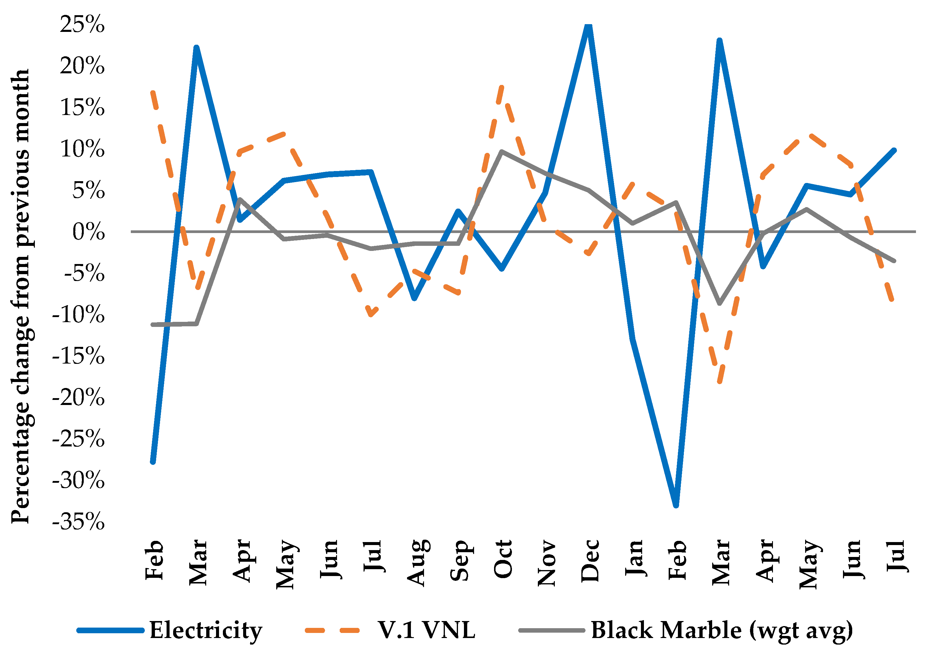
For the period from January 2020 to July 2021, national electricity consumption in China shows large monthly fluctuations (Figure 4). In February 2020, electricity demand was 28% lower than in the previous month, and in February 2021, it was 33% lower; in turn, March each year showed rebounds with monthly increases in electricity demand of 22–23%. The majority (two-thirds) of China’s electricity demand comes from the secondary (industrial) sector [55].
A big contributor to these February declines and March rebounds in total electricity use is factory closures during the Chinese New Year and Spring Festival Golden Week national holidays, which started on 25 January in 2020 and on 12 February in 2021. Notably, despite the depressing effect on electricity demand of the holiday period in 2020 being lengthened by lockdowns instituted in some areas to control the spread of COVID-19 [19], the ‘February-effect’ of a decline in electricity use was even greater in 2021, which had no lockdown but which had the holiday period fully within the month rather than spread between late January and February. Thus, in the aggregate, the effect of seasonal holidays on China’s electricity demand likely outweighs the effect of public health containment and closure measures. Even without the holiday-affected months of February and March, month-by-month changes in electricity consumption range from −13% to +25% and have an average absolute value of almost 8%.
The fluctuations in electricity consumption are not matched by monthly changes in the two NTL data products included in Figure 4: the monthly V.1 VNL cloud-free DNB composite and the weighted average of the Black Marble snow-free and snow-covered all-angles monthly composites. The V.1 VNL composite tends to show increases in NTL in months when total electricity use falls; the Pearson correlation coefficient between the monthly changes in total electricity use and the monthly changes in NTL is −0.52. This negative relationship also holds for components of total electricity use, with correlations of −0.46 between changes in the V.1 VNL monthly composite and monthly changes in secondary sector electricity use and of −0.42 with monthly changes in residential electricity use. For the Black Marble monthly composite, the correlation coefficients are −0.11 with respect to changes in either total or secondary sector electricity use and −0.32 for changes in residential electricity use. If only the snow-free monthly composite is used, rather than the weighted average of snow-free and snow-covered composites, the correlations with changes in NTL data are hardly altered, at −0.08 for monthly changes in total electricity use and −0.34 for the monthly changes in residential electricity use.

4. Discussion

In this paper, we have used a comprehensive and updated set of annual nighttime lights composites from DMSP and two VIIRS products: V.2 VNL and Black Marble. In the core analysis, we examined relationships of NTL data with county-level economic activity in China over the 2012 to 2019 period, using an estimation framework that lets us separately examine cross-sectional relationships of luminosity with levels of economic activity and time-series changes in economic activity and in NTL data. We also link to prior results for China by examining relationships one step higher in the administrative hierarchy, at the prefectural level. Our aim in using multi-source NTL data, and multiple levels of the administrative hierarchy, stems from a concern that the most widely cited validation studies that assess NTL data as a proxy for economic activity are for DMSP data with aggregated spatial units, such as nations or the first sub-national level. However, applied studies increasingly use NTL data to proxy for economic activity at very local levels, such as the third sub-national level (e.g., counties) and below, and also increasingly use VIIRS data.
The previous evidence for China that uses the within estimator on DMSP data at the prefectural level, in order to estimate the elasticity of annual GDP changes with respect to annual changes in NTL data, provides elasticity estimates of about 0.25 [37,42]. These prior estimates used 1992–2005 and 2000–12 time series. Given that we estimate an elasticity of 0.28 using annual changes in DMSP data (with standard error of 0.06) at prefectural level (in Table 4), for the 2012 to 2019 period, it suggests that the lights-GDP elasticity has not shifted over time as this estimate is very close to the results for China in prior periods. Moreover, this estimate is very similar to the elasticity of 0.3 reported from DMSP data at the country level in the most widely cited validation study [5]. Given this proliferation of GDP-lights elasticity estimates of about 0.3, a common procedure in the applied literature is to estimate effects of the studied treatment (such as a disaster or a policy intervention) on the change in NTL data and to then use a GDP-lights elasticity of 0.3 (or thereabouts) from the literature to convert the estimated treatment-lights effect into an effect in terms of economic activity [15,17,40].
The apparent temporal stability of the GDP-lights elasticity is reassuring because it suggests that one can apply existing elasticity estimates, even if from a prior time period, to convert a contemporary estimate of the effect of treatment on nighttime lights into an estimate of the effect of treatment on GDP. However, a problem with this procedure that our findings highlight is that elasticities do not appear to be invariant to either the source of NTL data or (at least for DMSP data) to the level within the spatial hierarchy at which they are estimated. In terms of the spatial level, when we use annual changes in DMSP data and in GDP data at the county level, the elasticity is only 0.11 (Table 3), despite these data being the same as those used at the prefectural level where the elasticity appears to be 0.28. If long-differences are used, the DMSP-derived elasticities are also far higher when estimated at the prefectural level rather than the county level. Consequently, studies that combine an existing GDP-lights elasticity (estimated with more aggregated data) from the literature with their own estimate of the effect of a treatment on luminosity at a lower spatial level, such as at the county level, are likely to overstate the impacts of the treatment in terms of economic activity. For example, studies using DMSP data at the city level and converting an estimated treatment effect in terms of luminosity into economic growth terms by using an assumed GDP-lights elasticity of 0.38 [22], or studies at the sub-district (third sub-national level) that assume that the GDP-lights elasticity ranges from 0.31 to 0.47 [17], are likely to overstate the treatment impacts on GDP changes.
In terms of the source of NTL data, at either the county level or the prefectural level, the elasticities of annual changes in GDP with respect to annual changes in VIIRS nighttime lights are far below 0.3 and would be better approximated by using a value of 0.1. Therefore, as applied studies increasingly switch from using DMSP data to using VIIRS data, the elasticities from existing validation studies based on DMSP data may no longer be applicable. Notably, the elasticity of 0.1, found by the within estimator with China’s annual county and prefectural-level data, is very similar to what is found at the county level for the United States [30]. If this low value of the GDP-luminosity elasticity holds more generally (and noting that the within R2 values are close to zero), then annual changes in NTL data may not be a good proxy for annual changes in local economic activity even though the levels of NTL data are good proxies for the levels of GDP. In other words, estimates of a treatment impact on changes in NTL data may be less informative of impacts on economic growth. Our analyses of China’s monthly electricity use fluctuations in Figure 4 also show that changes in NTL data do not appear to be very good predictors of short-term changes in economic activity, at least in this particular context.
A general comment, which ties together the discussion of multi-source NTL data and multiple levels of spatial units in the administrative hierarchy, is that findings from validation studies in different settings, with different NTL data products, or at different levels of spatial aggregation, may not translate to other settings. Evidence for this point also comes through in Table 5, where elasticities of the change in GDP with respect to the change in NTL data vary with population density for all of the VIIRS data products that we use. In other words, an elasticity estimated from a densely populated urban area is unlikely to be suitable for a sparsely populated rural area [35], which is problematic because it is the sparsely populated rural areas where alternative approaches to the measurement of economic activity are most needed, given that these settings tend to be some of the most difficult places to gather data through traditional approaches, such as face-to-face surveys of rural enterprises and households.

5. Conclusions

In this paper, we have examined the question of how good are nighttime lights data for studying differences in economic activity between areas and for studying the temporal changes in economic activity within areas. In line with findings elsewhere, the nighttime lights data did far worse at predicting time-series changes in economic activity than at predicting differences in economic activity cross-sectionally. The predictive power is roughly 50-times greater for cross-sectional differences in economic activity than it is for modeling time-series changes in activity. The weak relationships between changes in nighttime lights data and changes in economic activity raise issues for interpreting applied studies that show effects of a treatment (e.g., a shock or intervention) on changes in nighttime lights. While such effects are interesting, they are unlikely to proportionately translate into economic activity terms, and it is economic activity rather than luminosity per se that is likely to be of interest to policymakers.
A reasonable summary of our estimates is that annual changes in county-level GDP in China have an elasticity of about 0.1 with respect to annual changes in NTL data. Interestingly, this elasticity is very similar to county-level results for the United States, even though the growth in nighttime lights in China has been far faster than in the United States over the period studied. It will be an important task for future research to find other settings with benchmark economic activity data for lower-level units in the administrative hierarchy, such as counties, in order to assess whether a GDP-lights elasticity of 0.1 for annual changes holds more widely. If elasticities with VIIRS data are found to be far lower than the values of 0.3 or 0.4 reported in widely cited validation studies using DMSP data at national or first sub-national levels, it will suggest a need to revise the interpretation of various applied studies that use elasticity values from the literature to convert their findings into economic activity terms.
Beyond these broad conclusions, there are also some conclusions that may be more specific to China. In places where there are a non-trivial number of snow-covered nights per year, taking account of radiance measurements on these nights, as well as on the snow-free nights, is helpful for modeling annual GDP (which, by definition, measures economic activity in both snow-free and snow-covered periods). In particular, using the Black Marble data products, and including the snow-free and snow-covered composites, allowed us to have coverage of the greatest number of nights per year (about 10% more than just using a snow-free Black Marble composite and from 20–50% more nights per year than using V.2 VNL data). The resulting model with the weighted average of the Black Marble composites appeared to be closer to the truth than were other models of GDP changes, according to the non-nested testing. It will require further testing in other settings to see if these apparent advantages of the Black Marble data products hold more widely.

Author Contributions

Conceptualization and methodology, X.Z. and J.G.; Software, validation, data curation, and GIS analysis, X.Z.; Econometric analysis, preparation of original draft, and revision editing, J.G.; Visualization, X.Z.; Project administration and funding acquisition, J.G. All authors have read and agreed to the published version of the manuscript.

Funding

This research was funded by Marsden Fund Grant UOW-1901.

Institutional Review Board Statement

Not applicable.

Informed Consent Statement

Not applicable.

Data Availability Statement

The county-level GDP data are available from various issues of the China Statistical Yearbook and from the National Bureau of Statistics at http://www.stats.gov.cn/. DMSP stable lights annual composites are from: https://eogdata.mines.edu/products/dmsp/#download. The annual VNL V.2 data used in this study are available for download from the Earth Observation Group of the Colorado School of Mines at https://eogdata.mines.edu/products/vnl/#annual_v2. The annual Black Marble VIIRS data used in this study are available for download from: https://ladsweb.modaps.eosdis.nasa.gov/achive/allData/5000/VNP46A4/. All websites were last accessed on 28 January 2022.

Acknowledgments

We are grateful to Geua Boe-Gibson for assistance that helped to improve this paper. We also acknowledge the use of images and data processing by the Earth Observation Group, Payne Institute for Public Policy, Colorado School of Mines.

Conflicts of Interest

The authors declare no conflict of interest.

References

  1. Elvidge, C.D.; Baugh, K.E.; Kihn, E.A.; Kroehl, H.W.; Davis, E.R.; Davis, C.W. Relation between satellite observed visible-near infrared emissions, population, economic activity and electric power consumption. Int. J. Remote Sens. 1997, 18, 1373–1379. [Google Scholar] [CrossRef]
  2. Doll, C.N.; Muller, J.P.; Morley, J.G. Mapping regional economic activity from night-time light satellite imagery. Ecol. Econ. 2006, 57, 75–92. [Google Scholar] [CrossRef]
  3. Sutton, P.C.; Elvidge, C.D.; Ghosh, T. Estimation of Gross Domestic Product at sub-national scales using nighttime satellite imagery. Int. J. Ecol. Econ. Stat. 2007, 8, 5–21. [Google Scholar]
  4. Chen, X.; Nordhaus, W.D. Using luminosity data as a proxy for economic statistics. Proc. Natl. Acad. Sci. USA 2011, 108, 8589–8594. [Google Scholar] [CrossRef] [PubMed] [Green Version]
  5. Henderson, J.V.; Storeygard, A.; Weil, D.N. Measuring economic growth from outer space. Am. Econ. Rev. 2012, 102, 994–1028. [Google Scholar] [CrossRef] [PubMed] [Green Version]
  6. Shi, K.; Yu, B.; Huang, Y.; Hu, Y.; Yin, B.; Chen, Z.; Chen, L.; Wu, J. Evaluating the ability of NPP-VIIRS nighttime light data to estimate the gross domestic product and the electric power consumption of China at multiple scales: A comparison with DMSP-OLS data. Remote Sens. 2014, 6, 1705–1724. [Google Scholar] [CrossRef] [Green Version]
  7. Jing, X.; Shao, X.; Cao, C.; Fu, X.; Yan, L. Comparison between the Suomi-NPP Day-Night Band and DMSP-OLS for correlating socio-economic variables at the provincial level in China. Remote Sens. 2016, 8, 17. [Google Scholar] [CrossRef] [Green Version]
  8. Zhao, M.; Cheng, W.; Zhou, C.; Li, M.; Wang, N.; Liu, Q. GDP spatialization and economic differences in South China based on NPP-VIIRS nighttime light imagery. Remote Sens. 2017, 9, 673. [Google Scholar] [CrossRef] [Green Version]
  9. Wang, X.; Rafa, M.; Moyer, J.; Li, J.; Scheer, J.; Sutton, P. Estimation and mapping of sub-national GDP in Uganda using NPP-VIIRS imagery. Remote Sens. 2019, 11, 163. [Google Scholar] [CrossRef] [Green Version]
  10. Liu, H.; He, X.; Bai, Y.; Liu, X.; Wu, Y.; Zhao, Y.; Yang, H. Nightlight as a proxy of economic indicators: Fine-grained GDP inference around mainland China via attention-augmented CNN from daytime satellite imagery. Remote Sens. 2021, 13, 2067. [Google Scholar] [CrossRef]
  11. Clark, H.; Pinkovskiy, M.; Sala-I-Martin, X. China’s GDP growth may be understated. China Econ. Rev. 2020, 62, 101243. [Google Scholar] [CrossRef] [Green Version]
  12. Lee, Y.S. International isolation and regional inequality: Evidence from sanctions on North Korea. J. Urban Econ. 2018, 103, 34–51. [Google Scholar] [CrossRef]
  13. Marx, A.; Rogers, M. Analysis of Panamanian DMSP/OLS nightlights corroborates suspicions of inaccurate fiscal data: A natural experiment examining the accuracy of GDP data. Remote Sens. Appl. Soc. Environ. 2017, 8, 99–104. [Google Scholar] [CrossRef]
  14. Nguyen, C.N.; Noy, I. Measuring the impact of insurance on urban earthquake recovery using nightlights. J. Econ. Geogr. 2020, 20, 857–877. [Google Scholar] [CrossRef]
  15. Kocornik-Mina, A.; McDermott, T.K.; Michaels, G.; Rauch, F. Flooded cities. Am. Econ. J. Appl. Econ. 2020, 12, 35–66. [Google Scholar] [CrossRef]
  16. Zhao, N.; Liu, Y.; Hsu, F.; Samson, E.; Letu, H.; Liang, D.; Cao, G. Time series analysis of VIIRS-DNB nighttime lights imagery for change detection in urban areas: A case study of devastation in Puerto Rico from hurricanes Irma and Maria. Appl. Geog. 2020, 120, 102222. [Google Scholar] [CrossRef]
  17. Heger, M.P.; Neumayer, E. The impact of the Indian Ocean tsunami on Aceh’s long-term economic growth. J. Dev. Econ. 2019, 141, 102365. [Google Scholar] [CrossRef]
  18. Zhao, X.; Yu, B.; Liu, Y.; Yao, S.; Lian, T.; Chen, L.; Yang, C.; Chen, Z.; Wu, J. NPP-VIIRS DNB daily data in natural disaster assessment: Evidence from selected case studies. Remote Sens. 2018, 10, 1526. [Google Scholar] [CrossRef] [Green Version]
  19. Elvidge, C.; Ghosh, T.; Hsu, F.-C.; Zhizhin, M.; Bazilian, M. The dimming of lights in China during the COVID-19 pandemic. Remote Sens. 2020, 12, 2851. [Google Scholar] [CrossRef]
  20. Xu, G.; Xiu, T.; Li, X.; Liang, X.; Jiao, L. Lockdown induced night-time light dynamics during the COVID-19 epidemic in global megacities. Int. J. Appl. Earth 2021, 102, 102421. [Google Scholar] [CrossRef]
  21. Roberts, M. Tracking economic activity in response to the COVID-19 crisis using nighttime lights—The case of Morocco. Dev. Eng. 2021, 6, 100067. [Google Scholar] [CrossRef]
  22. Eberhard-Ruiz, A.; Moradi, A. Regional market integration in East Africa: Local but no regional effects? J. Dev. Econ. 2019, 140, 255–268. [Google Scholar] [CrossRef]
  23. Chodorow-Reich, G.; Gopinath, G.; Mishra, P.; Narayanan, A. Cash and the economy: Evidence from India’s demonetization. Q. J. Econ. 2020, 135, 57–103. [Google Scholar] [CrossRef]
  24. Henderson, J.V.; Squires, T.; Storeygard, A.; Weil, D. The global distribution of economic activity: Nature, history, and the role of trade. Q. J. Econ. 2018, 133, 357–406. [Google Scholar] [CrossRef] [PubMed]
  25. Goldblatt, R.; Heilmann, K.; Vaizman, Y. Can Medium-Resolution Satellite Imagery Measure Economic Activity at Small Geographies? Evidence from Landsat in Vietnam. World Bank Econ. Rev. 2020, 34, 635–653. [Google Scholar] [CrossRef]
  26. Asher, S.; Lunt, T.; Matsuura, R.; Novosad, P. Development research at high geographic resolution: An analysis of night-lights, firms and poverty in India suing the SHRUG open data platform. World Bank Econ. Rev. 2021, 35, 845–871. [Google Scholar] [CrossRef]
  27. Nordhaus, W.; Chen, X. A sharper image? Estimates of the precision of nighttime lights as a proxy for economic statistics. J. Econ. Geogr. 2015, 15, 217–246. [Google Scholar] [CrossRef]
  28. Elvidge, C.D.; Baugh, K.E.; Zhizhin, M.; Hsu, F.C. Why VIIRS data are superior to DMSP for mapping nighttime lights. Proc. Asia-Pac. Adv. Netw. 2013, 35, 62. [Google Scholar] [CrossRef] [Green Version]
  29. Chen, X.; Nordhaus, W.D. VIIRS nighttime lights in the estimation of cross-sectional and time-series GDP. Remote Sens. 2019, 11, 1057. [Google Scholar] [CrossRef] [Green Version]
  30. Gibson, J.; Boe-Gibson, G. Nighttime lights and county-level economic activity in the United States: 2001 to 2019. Remote Sens. 2021, 13, 2741. [Google Scholar] [CrossRef]
  31. Baugh, K.; Elvidge, C.D.; Ghosh, T.; Ziskin, D. Development of a 2009 stable lights product using DMSP-OLS data. Proc. Asia-Pac. Adv. Netw. 2010, 30, 114. [Google Scholar] [CrossRef]
  32. Elvidge, C.D.; Zhizhin, M.; Ghosh, T.; Hsu, F.-C.; Taneja, J. Annual time series of global VIIRS nighttime lights derived from monthly averages: 2012 to 2019. Remote Sens. 2021, 13, 922. [Google Scholar] [CrossRef]
  33. Román, M.; Wang, Z.; Sun, Q.; Kalb, V.; Miller, S.; Molthan, A.; Schultz, L.; Bell, J.; Stokes, E.; Pandey, B.; et al. NASA’s Black Marble nighttime lights product suite. Remote Sens. Environ. 2018, 210, 113–143. [Google Scholar] [CrossRef]
  34. Gibson, J. Better night lights data, for longer. Oxf. Bull. Econ. Stat. 2021, 83, 770–791. [Google Scholar] [CrossRef]
  35. Gibson, J.; Olivia, S.; Boe-Gibson, G.; Li, C. Which night lights data should we use in economics, and where? J. Dev. Econ. 2021, 149, 102602. [Google Scholar] [CrossRef]
  36. Hodler, R.; Raschky, P.A. Regional favoritism. Q. J. Econ. 2014, 129, 995–1033. [Google Scholar] [CrossRef]
  37. Storeygard, A. Farther on down the road: Transport costs, trade and urban growth in sub-Saharan Africa. Rev. Econ. Stud. 2016, 83, 1263–1295. [Google Scholar] [CrossRef] [Green Version]
  38. Tuttle, B.; Anderson, S.; Sutton, P.; Elvidge, C.; Baugh, K. It used to be dark here. Photogramm. Eng. Remote Sensing. 2013, 79, 287–297. [Google Scholar] [CrossRef]
  39. Abrahams, A.; Oram, C.; Lozano-Gracia, N. Deblurring DMSP nighttime lights: A new method using Gaussian filters and frequencies of illumination. Remote Sens. Environ. 2018, 210, 242–258. [Google Scholar] [CrossRef]
  40. Villa, J. Social transfers and growth: Evidence from luminosity data. Econ. Dev. Cult. Chang. 2016, 65, 39–61. [Google Scholar] [CrossRef]
  41. Ji, X.; Li, X.; He, Y.; Liu, X. A simple method to improve estimates of county-level economics in China using nighttime light data and GDP growth rate. ISPRS Int. J. Geoinf. 2019, 8, 419. [Google Scholar] [CrossRef] [Green Version]
  42. Gibson, J.; Olivia, S.; Boe-Gibson, G. Night lights in economics: Sources and uses. J. Econ. Surv. 2020, 34, 955–980. [Google Scholar] [CrossRef]
  43. National Bureau of Statistics (NBS). China Statistical Yearbook (County-Level) [M]; China Statistics Press: Beijing, China, 2013–2020. [Google Scholar]
  44. National Bureau of Statistics (NBS). China City Statistical Yearbook [M]; China Statistics Press: Beijing, China, 2013–2020. [Google Scholar]
  45. National Bureau of Statistics (NBS). Beijing Statistical Yearbook [M]; China Statistics Press: Beijing, China, 2013–2020. [Google Scholar]
  46. Ghosh, T.; Baugh, K.; Elvidge, C.; Zhizhin, M.; Poyda, A.; Hsu, F.-C. Extending the DMSP Nighttime Lights Time Series beyond 2013. Remote Sens. 2021, 13, 5004. [Google Scholar] [CrossRef]
  47. Elvidge, C.D.; Baugh, K.; Zhizhin, M.; Hsu, F.C.; Ghosh, T. VIIRS night-time lights. Int. J. Remote Sens. 2017, 38, 5860–5879. [Google Scholar] [CrossRef]
  48. Wooldridge, J. Introductory Econometrics: A Modern Approach, 7th ed.; Cengage Publishing: Boston, MA, USA, 2020. [Google Scholar]
  49. Kim, B.; Gibson, J.; Chung, C. Using panel data to estimate income under-reporting by the self-employed. Manch. Sch. 2017, 85, 41–64. [Google Scholar] [CrossRef] [Green Version]
  50. Greene, W. Econometric Analysis, 4th ed.; Prentice Hall Publishing: Hoboken, NJ, USA, 2000. [Google Scholar]
  51. Vuong, Q. Likelihood ratio tests for model selection and non-nested hypotheses. Econometrical 1989, 57, 307–333. [Google Scholar] [CrossRef] [Green Version]
  52. Hu, X.; Huang, X. A novel locally adaptive method for modeling the spatiotemporal dynamics of global electric power consumption based on DMSP-OLS nighttime stable light data. Appl. Energy 2019, 240, 778–792. [Google Scholar] [CrossRef]
  53. Zhao, F.; Ding, J.; Zhang, S.; Luan, G.; Song, L.; Peng, Z.; Du, Q.; Xie, Z. Estimating rural electric power consumption using NPP-VIIRS night-time light, toponym and POI data in ethnic minority areas of China. Remote Sens. 2020, 12, 2836. [Google Scholar] [CrossRef]
  54. Sahoo, S.; Gupta, P.; Srivastav, S. Comparative analysis between VIIRS-DNB and DMSP-OLS night-time light data to estimate electric power consumption in Uttar Pradesh, India. Int. J. Remote Sens. 2020, 41, 2565–2580. [Google Scholar] [CrossRef]
  55. National Energy Administration (NES). Available online: http://www.nea.gov.cn/ (accessed on 5 November 2021).
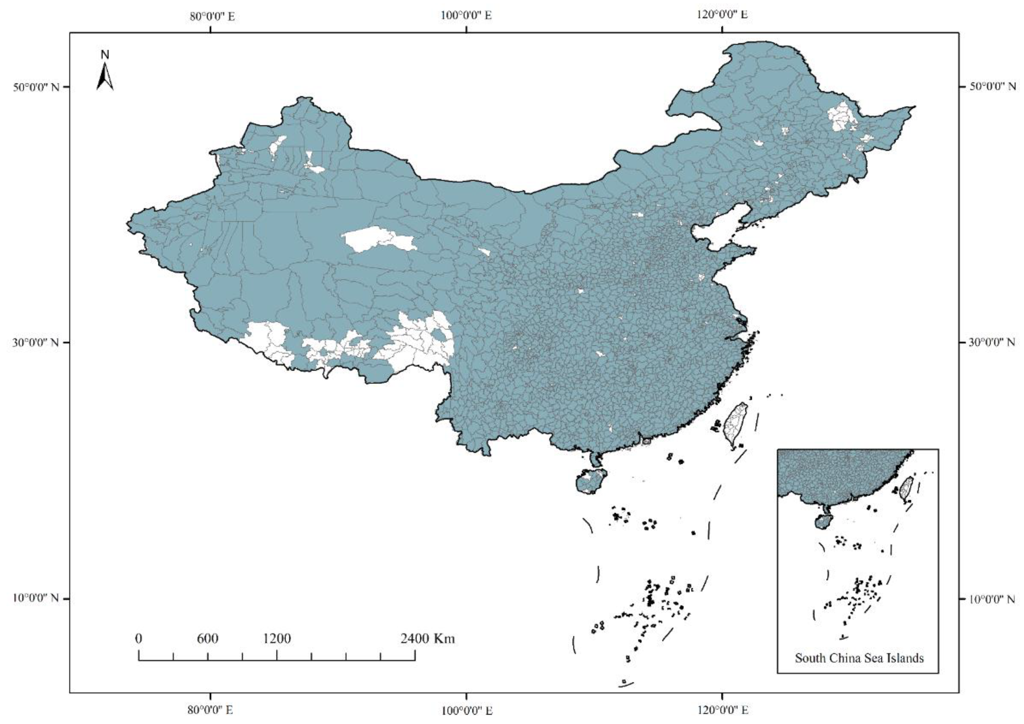
Figure 1. County-level spatial units in China (no GDP data if blank).
Remotesensing 14 01282 g001
Figure 2. County-level average ratios of the number of snow-covered nights to the total number of nights with Black Marble data used for annual composites.
Remotesensing 14 01282 g002
Figure 3. Average number of nights per year included in NTL composites for China.
Remotesensing 14 01282 g003
Figure 4. Monthly changes in China’s electricity use and NTL composites: 2020–21.
Remotesensing 14 01282 g004
Table 1. Attributes of the various NTL data sources and data products.
DMSPV.2 VNLBlack Marble
Satellite/Sensor Attributes
OperatorUS DoDNASA/NOAA
Available years1992–20192012–2020
Spectral band0.5–0.9 μm0.5–0.9 μm
Orbit type and altitudePolar, 830 kmPolar, 830 km
Spatial resolution at nadir2.7 km742 m
Scan width3000 km3000 km
Revisit time12 h12 h
Pixel saturationSaturatedNot saturated
On-board calibrationNoYes
Data Products
Creator of annual compositesEOGEOGNASA
Spatial resolution30 arc second15 arc second15 arc second
TiledNoNoYes, 648 tiles
Masking of ephemeral light sourcesNoYesYes
Stray-light correctionNoYes, from 2014Yes
User control over angle of detectionNoNoYes
Treatment of snowNoNoYes
Note: DoD is Department of Defense, EOG is Earth Observation Group.
Table 2. Descriptive statistics and correlation coefficients.
Matrix of Correlation Coefficients
MeanStd DevDMSPV.2 VNLBMsfBMwa
DMSP8.5261.176
V.2 VNL7.9991.2470.850
BMsf10.4781.2540.7910.872
BMwa10.5001.2260.8570.9640.903
GDP4.9501.2660.6350.7300.6870.740
Notes: Based on n = 21,256 observations (2657 county-level units each observed 8 times). All variables are in logarithms. BMsf and BMwa are Black Marble snow-free and weighted average.
Table 3. Relationships between multi-source NTL and county-level GDP: within and between-estimator results.
Independent Variables and Summary StatisticsAnnual NTL Data Product
DMSP Stable
Lights
V.2 VNL
Masked Average
Black Marble
Snow-Free
Black Marble
Weighted Average
Within-estimator, for annual GDP changes within each county
ln (sum of lights)0.109 ***0.067 ***0.022 ***0.124 ***
(0.010)(0.015)(0.004)(0.016)
Year fixed effectsYesYesYesYes
County fixed effectsYesYesYesYes
R-squared (Within)0.0140.0040.0020.011
Between-estimator, for average GDP differences between counties
ln (sum of lights)0.786 ***0.764 ***0.834 ***0.780 ***
(0.015)(0.013)(0.014)(0.013)
R-squared (Between)0.5000.5600.5870.579
Notes: Results are based on a strongly balanced panel of 2657 county-level units, observed each year from 2012 to 2019, giving n = 21,256 observations. Standard errors are in parentheses (clustered by county for the within-estimator results), *** p < 0.01.
Table 4. Relationships between multi-source NTL and prefectural-level GDP: within and between-estimator’s results.
Independent Variables and Summary StatisticsAnnual NTL Data Product
DMSP Stable
Lights
V.2 VNL
Masked Average
Black Marble
Snow-Free
Black Marble
Weighted Average
Within-estimator, for annual GDP changes within each prefecture
ln (sum of lights)0.275 ***0.0380.025 *0.135 **
(0.061)(0.046)(0.013)(0.068)
Year fixed effectsYesYesYesYes
County fixed effectsYesYesYesYes
R-squared (Within)0.0140.0000.0010.002
Between-estimator, for average GDP differences between prefectures
ln (sum of lights)0.965 ***0.924 ***0.995 ***0.947 ***
(0.054)(0.047)(0.047)(0.046)
R-squared (Between)0.4790.5270.5620.552
Notes: Based on a strongly balanced panel of 347 prefectural-level units, observed each year from 2012 to 2019, giving a sample of n = 2776 observations. Standard errors are in parentheses (clustered at prefectural level for the within-estimator results), * p < 0.10, ** p < 0.05, *** p < 0.01.
Table 5. Effects of population density on the relationship between NTL variables and county-level GDP.
Independent Variables and Summary StatisticsAnnual NTL Data Product
DMSP Stable
Lights
V.2 VNL
Masked Average
Black Marble
Snow-Free
Black Marble
Weighted Average
Within-estimator, for annual GDP changes within each county
ln (sum of lights)0.111 ***0.078 ***0.021 ***0.139 ***
(0.011)(0.015)(0.004)(0.016)
ln (sum of lights) × density0.0050.041 ***0.004 **0.063 ***
(0.011)(0.011)(0.002)(0.018)
Year fixed effectsYesYesYesYes
County fixed effectsYesYesYesYes
R-squared (Within)0.0140.0050.0020.012
Between-estimator, for average GDP differences between counties
ln (sum of lights)0.767 ***0.736 ***0.805 ***0.753 ***
(0.014)(0.013)(0.014)(0.013)
ln (sum of lights) × density0.0160.0140.0090.013
(0.020)(0.019)(0.022)(0.019)
R-squared (Between)0.5580.5740.5990.592
Notes: Density is in standard deviation units. Between-estimator specification also includes density as a level term, but coefficients were always insignificantly different from zero, so are not reported (for within-estimator results, the density variable is time-invariant, and so the level term drops out). ** p < 0.05, *** p < 0.01. For other notes, see Table 3.
Publisher’s Note: MDPI stays neutral with regard to jurisdictional claims in published maps and institutional affiliations.