Abstract
Lately, generative adversarial networks (GAN)-based methods have drawn extensive attention and achieved a promising performance in the field of hyperspectral anomaly detection (HAD) owing to GAN’s powerful data generation capability. However, without considering the background spatial features, most of these methods can not obtain a GAN with a strong background generation ability. Besides, they fail to address the hyperspectral image (HSI) redundant information disturbance problem in the anomaly detection part. To solve these issues, the unsupervised generative adversarial network with background spatial feature enhancement and irredundant pooling (BEGAIP) is proposed for HAD. To make better use of features, spatial and spectral features union extraction idea is also applied to the proposed model. To be specific, in spatial branch, a new background spatial feature enhancement way is proposed to get a data set containing relatively pure background information to train GAN and reconstruct a more vivid background image. In a spectral branch, irredundant pooling (IP) is invented to remove redundant information, which can also enhance the background spectral feature. Finally, the features obtained from the spectral and spatial branch are combined for HAD. The experimental results conducted on several HSI data sets display that the model proposed acquire a better performance than other relevant algorithms.
1. Introduction
A hyperspectral image (HSI) is viewed as a 3-D matrix with spectral and spatial dimensions. The former contains a large amount of spectral information with a high resolution and the latter can provide rich structure information [1]. Depending on the abundant spatial-spectral feature, HSI has received attention from relevant research fields, including classification [2,3,4], spectral unmixing [5], and detection task [6]. Based on these information processing methods, HSI has been applied in military, food quality, safety, and agriculture [7]. In particular, the hyperspectral detection task has been a hot spot, which is divided into anomaly and target detection [8,9]. Target detection is a supervised learning way with a training set that needs a considerable amount of prior information. Anomaly detection (AD), which finds pixels or pixels region different from their surroundings, is also called hyperspectral anomaly detection (HAD) [10,11,12].
HAD is popularly supported by experts and extensively used in various fields because it does not need prior information. In the past 20 years, many classical algorithms have come out. The most well-known Reed–Xiaoli (RX) algorithm [13] supposes that the background obeys the multivariate Gaussian distribution. Anomalies are judged by computing Mahalanobis distance between each test pixel and the background reconstructed. Then many RX-based algorithms, including the kernel RX (KRX) [14] and local RX (LRX) [15], are put forward to enhance the detection effect. Nevertheless, the background model mean and covariance matrix calculated by the RX-based methods in a local or whole image region are inevitably mixed by the anomaly.
The representation-based approaches are also widely used in HAD. According to the hypothesis that the background has the low-rank characteristics, it can be linearly represented by the background dictionary. How to construct the dictionary is the vital part of relevant algorithms and some efficient reconstruction methods have also appeared, such as CRD [16] and LRASR [17]. However, the noise pixel in an image is not taken into account by the representation-based algorithms, which only decompose the original data into the background and abnormal pixel matrix. Hence, many noise pixels would be mistakenly identified as anomalies, increasing the AD false alarm rate. PAB-DC [18], on a basis of the construction of potential anomaly, and background dictionary, decomposes the original HSI into three parts: background, anomaly and noise. The background and anomaly dictionary is constructed, respectively, to linearly represent the corresponding image part. Then the noise in HSI is separated from HSI. Although the high false alarm rate problem is addressed in a way, the process is complicated. Unfortunately, many tasks are consumed to conduct the theoretical derivation of mathematical formulas and the performance has not been greatly improved.
The data processing methods based on deep neural networks and machine learning [19,20,21] show great advantage in the complex data processing, requiring researchers to focus on model and parameters design. These data processing ways can solve the issue that representation-based methods consume much power. Recently, with the continuous development of computer hardware equipment and relevant theoretical knowledge, AD technologies based on deep neural networks have made rapid progress [22,23]. The auto-encoder (AE) [24] is taken as the model core by most of these methods [25,26]. However, the generation ability of AE is poor. The neural network reconstructs the background by learning the distribution of original HSI pixels, then matrix decomposition is employed to obtain a residual image where the background is suppressed while the anomaly is highlighted. For the sake of enhancing the ability of reconstruction, researchers also applied the idea of generative adversarial networks (GAN) [27] to the mentioned network, making the AE a generator and adding a discriminator. The former deceives the latter while the latter discern the former. By means of improving the generalization capacity of neural networks through adversarial learning, these methods [25,26] have significantly improved the performance of HAD. Yet, the background spatial feature is not taken into consideration by the GAN-based network in [25,26], which would receive a GAN with a weak reconstruction ability for background. Hence, the goal of acquiring the GAN with a strong background generalization ability is not achieved. To tackle this matter, a new way of gaining a training set with a background spatial feature enhancement (BE) is raised according to the theory that background energy in each band have a bigger discrimination degree [25]. We group bands and select the representative band in each group in accordance with an energy discrimination degree, so that the training data set contains more pure background spatial information. The targeted GAN network can be trained by learning more pure background features. Besides, the generation capability of GAN is not stable. Thereby, some false background pixels would be generated in the reconstructed image. It leads to the appearance of false anomalies in the residual images compared to the initial HSI, which is not beneficial to the HAD in the subsequent process. To solve this problem, some strong constrained functions are proposed on the GAN networks. The contrastive learning also has great development potential [28,29]. Additionally, the AD part of the above deep neural network algorithms [25,26] is disturbed by HSI redundant information. Focusing on this issue, the irredundant pooling (IP) is proposed.
To detect a hyperspcetral image anomaly better, an unsupervised generative adversarial network with background enhancement and irredundant pooling (BEGAIP) is proposed by us. HSI has abundant spectral and certain spatial features, so spatial and spectral union detection is proposed for HAD. From the view of HAD, HSI consists of two kinds of pixels: background and anomaly. Hence, the background-anomaly separation idea is integrated into the spatial and spectral anomaly detection branch of our model. In the spatial branch, considering that background pixels obey Gaussian distribution and powerful data generation of GAN, BE-constrained two GANs are proposed to reconstruct a background image. The first GAN is aimed at utilizing HSI pixels to generate a low dimension image obeying Gaussian distribution, which means the low dimension background features map is extracted. Besides, in order to make the background features in the extracted feature map denser, BE is proposed by us to enhance the background spatial features in HSI. Therefore, the second GAN can generate a background image well by making use of the background features map obtained by the former. However, the GANs are not stable, some constrained functions are proposed and imposed to prevent them from generating false background pixels. Of course, the constrained functions can moderate, however not solve the unstability problem thoroughly. Thus, there is the appearance of false anomalies in the residual image because of false background pixels produced by reconstruction networks. So, some morphological operations [30] and PCA [31] are used to improve the spatial detection result. In the spectral branch, the Mahalanobis distance is used to detect spectral anomalies. Given the characteristic that HSI has abundant spectral information but slight redundancy, the irredundant pooling (IP) is proposed to protect spectral anomaly detection from redundant information disturbance. The spectral and spatial anomaly detection maps are fused as the final HAD result.
There are four contributions of the article, which are described below.
- Different from the traditional way, which only considers a pixel spectral value in network training, the BE is proposed to prepare for training data sets. In this part, we adopt the principle that the background energy in each band have a bigger discrimination degree than anomaly.
- The IP is invented in the spectral branch. We apply the grouping max pooling to eliminate the redundant information while highlighting the available feature as much as possible.
- Some strong constrained functions are imposed on the GAN, aimed at making the networks more stable to reconstruct a hyperspectral background image.
- A spectral-spatial joint way, processing the HSI rather than residual image, is integrated in the algorithm proposed to obtain the combination detection result, through which we can make the best use of data.
The structure of the article is arranged as follows. In Section 2, related work including the AE and GAN model is introduced. The BEGAIP model proposed for HAD is expatiated by Section 3. Section 4 demonstrates the experimental results and analysis. Some investigations are discussed in Section 5. Finally, this article is concluded in Section 6.
2. Related Work
In this part, the base components of the model BEGAIP proposed by us, including autoencoder (AE) and generative adversarial networks (GAN), are described.
2.1. Autoencoder (AE)
An automatic encoder (AE) is a neural network used for data generation, which is aimed to reconstruct the data with the distance as small as possible from the original data. It performs backpropagation [32] by minimizing the distribution law gap between the initial and data generated by AE. It consists of two parts: encoder and decoder. The former maps the original data into low-dimensional data. The reduced dimension data contains many important features in initial data and discard invalid information. The latter restores the data generated by the encoder into data consistent with the dimension of the original data. The latent feature layer is the part between the encoder and decoder, which is used to temporarily store low-dimensional data. The formula of the encoder is as follows:
where corresponds to the encoder function, x is the input data of the network, and w and b are the weight and offset coefficient, respectively. z is the low-dimensional data after mapping, which contains important features in x. Similarly, the decoder function can also be expressed by the formula:
where is the function corresponding to the decoder, and and are the weight and offset coefficient of the decoder, is the data generated by the decoder by making use of z. and the original data x contain a large amount of the same information, which is achieved by the following constraints:
where represents the reconstruction error in the whole process, which is represented by an norm. In order to minimize , it is necessary to propagate back loss to continuously update the network parameters {} to make the input and output data as similar as possible while discarding ineffective features.
2.2. Generative Adversarial Networks (GAN)
GANs is a neural network model proposed by Lan Goodflow in 2014 [27], which is a good generative model [33,34]. Recently, it has shown great advantages in unsupervised application scenarios with complex data distribution. GAN is composed of a Generator (G) and a Discriminator (D). The G aims to learn the input data distribution and generate data that is as close to them as possible. Then, the initial samples and reconstructed samples are given to D. It spares no effort to recognize the false sample and gives the lower score. The goal of G is to deceive the D while the task of the D is to identify the deception of the former. It means that they continue to optimize the parameters of their own through adversarial learning. The learning process can be described as the following function:
where is a classical loss function [35], x and z are the input data and the rand noise data used by the G, respectively, and are the distribution laws of x and z. log and E are logarithms and expectations in statistics. The training process of G and D is carried out alternately and the result of one training is obtained according to Equation (4). Maximum, from the perspective of D, manages to see through the deception. The D gives a higher score to the real sample but a lower score to the false sample generated by the G. Minimum, from the perspective of the G, successfully deceives the D. The D gives a lower score to the real sample while a higher score to the false sample generated by the G using noise data. Thus, in the periodical training process, we gain the best D when the expectation sum in Equation (4) reaches the maximum. Similarly, optimal G is obtained when the minimum appears.
3. Methodology
In this part, the model BEGAIP proposed is introduced in detail by including three parts. The overall framework is illustrated in Figure 1. Firstly, in the spatial branch, we propose the constrained GAN based on background spatial feature enhancement (BEGAN). It is used to obtain a GAN with a strong background image generation capability, which reconstructs the background matrix. Then the residual matrix with background suppressed and anomaly relatively highlighted is obtained by matrix decomposition. The spatial detection part is also proposed to improve the detection result. Secondly, the IP is presented in the spectral branch, then regularized Mahalanobis distance is applied to gain the spectral feature. Thirdly, the features extracted from the spectral and spatial branch are fused in proportion, and the synthesized image is used as the final HAD result.
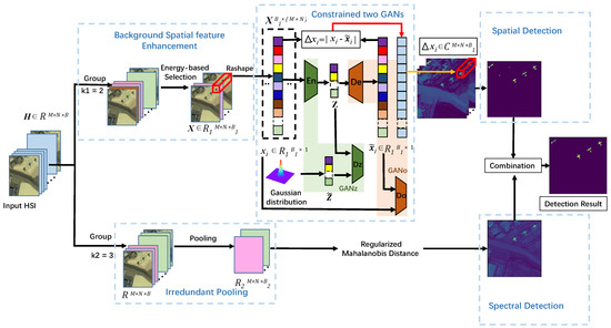
Figure 1.
The architecture of unsupervised generative adversarial network with background spatial feature enhancement and irredundant pooling (BEGAIP). It consists of five portions: background spatial feature enhancement, constrained two GANs (GANz, GANo), spatial detection, irredundant pooling, and regularized mahalanobis distance.
3.1. BEGAN-Based Spatial Anomaly Detection
The HSI spatial feature plays a significant part in HAD. In particular, in the detection effect picture, the anomaly area can not be accurately recognized without considering the spatial feature. To better apply background features to separate anomalies from the background in the spatial view, BEGAN-based spatial anomaly detection is proposed. It includes BE, constrained two GANs, and spatial detection. The algorithm details are as follows.
3.1.1. Background Spatial Feature Enhancement
HSI consists of background and anomaly pixels. In particular, the number of background pixels is far more than the anomalies’ pixels. Thus, compared with anomaly pixels, background pixels energy value has a bigger discrimination degree. From a spatial point of view, the larger the gray value sum of all pixels element in this band, the more background spatial information contained in this band [25]. On the contrary, this band contains relatively more anomaly features. Thus, in the BEGAIP spatial branch, the HSI are grouped, where there are bands, then the band with the largest gray value sum is chosen in each group. In other words, the band containing as much spatial background information as possible is selected. These bands form a new data set . The specific structure is shown by the background spatial feature enhancement in Figure 1, where M, N, and , which is equal to B divided by are the height, width, and band number of the new HSI data set.
3.1.2. Constrained Two GANs
In this section, we focus on constrained two GANs. The traditional unsupervised learning methods ignore background spatial features in the training. Therefore, the network will only learn the background pixel gray values. Besides, the GAN is not stable. Hence, there are some false background pixels in the image reconstructed by the GAN with a weak background generalization ability. Therefore, the abnormal information contained in the residual image obtained by matrix decomposition, Equation (5), is far more than the initial HSI. The matrix decomposition formula is defined as follows:
where , is a B-band pixel and n is the number of pixels in the HSI, is the background pixel matrix reconstructed by the network, and is the anomalous pixel matrix. In traditional neural network methods, a considerable amount of false anomalous information, which is not contained in the X, appears in A.
To address the issue, we propose a new constrained GAN training method based on BE. According to the characteristic that GAN tends to learn the distribution law of the samples whose number is the largest in the training data and the number of background pixel is far more than the anomaly pixel’s, if the new HSI set is used for training, the GAN obtained can reconstruct the background image. As recommended by [25], the original AE is modified by adding discriminator Dz and discriminator Do to the latent feature layer and output layer of the decoder, respectively, which constitutes two GANs, denoted as GANz and GANo. In line with the composition of the GAN model, the encoder (En) and decoder (De) are generators of GANz and GANo, respectively, and Dz and Do are discriminators of GANz and GANo, respectively. In addition, the encoder (En) and discriminator Dz form the GANz, decoder (De) and discriminator Do consist of the GANo. Similar to the anomaly detection algorithm based on RX, we also assume that background pixels in HSI data sets conform to the Gaussian distribution, however anomalous pixels do not. The discriminator Dz regards the noise obeying the Gaussian distribution as the real sample and the background pixels also conform to Gaussian distribution. Thus, GANz can extract the background pixels’ features. The GANo is applied to generate background pixels by utilizing background features obtained by GANz. Therefore, the union of GANz and GANo would help reconstruct the background image better. The new HSI data set is reshaped into two dimensional matrix , where the number of rows and columns are the number of bands and pixels. A pixel vector is a training data sample. Generator En consists of 3 fully connected layers {} followed by Leaky Relu [36] with slope 0.2, where is the square root of . Discriminator Dz is made up of 3 fully connected layers {} followed by Leaky Relu with slope 0.2 and Dropout with default 0.1, whose final activation function is sigmoid. Generator De is composed of 3 fully connected layers {} followed by Leaky Relu with slope 0.2. Discriminator Do is formed by 3 fully connected layers {} followed by Leaky Relu with slope 0.2 and a dropout with a default of 0.1, whose final action function is also sigmoid. In addition, the learning rate is set to 0.0001. The more specific details of constrained two GANs components are depicted in Figure 2.
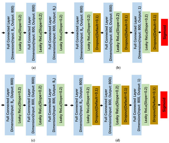
Figure 2.
The more specific details of constrained two GANs components. (a) Generator (En). (b) Discriminator (Dz). (c) Generator (De). (d) Discriminator (Do).
Additionally, to moderate GANs unstabitily and reconstruct the background image perfectly, spectral angle constraint (6), latent layer constrain (7), and reconstruction error (3) are added in the unsupervised network. Besides, the latent layer constrain (7) can make the network robust to noise in a way. The details are as illustrated in Figure 3. The spectral angle constraint is:
in Equation (6), represents the spectral angle constraint, and are the original and reconstructed pixel, respectively, and is the norm of the vector.
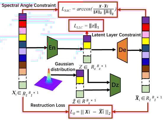
Figure 3.
The detailed information of spatial branch network loss.
Furthermore, constraint (7) is appended to the latent feature layer of AE. It is as follows:
where , z denote the latent layer constrain and low-dimension pixel vector produced by the encoder. Combining the constrain (3), (6) and (7), the loss in the training process of spatial branch network is defined as:
where is the total loss of the whole network, , , and are, respectively, the homologous proportionality coefficient.
Compared with the traditional unsupervised method, the network with can reconstruct the more accurate background matrix quickly and stably. The detailed process of BEGAN is described in Algorithm 1.
| Algorithm 1: Background spatial feature enhancement-based constrained two GANs training |
Input: HSI data set , group number Output: , , ,
|
3.1.3. Spatial Detection
Firstly, PCA is employed to select the band from the residual image. As the background is suppressed while the anomaly is enhanced, the band chosen contains the most anomaly information, denoted as . Then it is regarded as the base map of subsequent spatial detection.
Secondly, due to the unstable generation ability of GAN, some irregular background pixels are produced in the reconstructed image. It would lead to the matter that some sparsely distributed false anomaly exists in , increasing the detection false alarm rate. To solve the problem, morphological opening and closing operation are adopted to eliminate sporadic false anomalous pixels and smooth the boundary without changing the area of true anomalies in the . The details are depicted in Figure 4. Combining the morphology open with the close operation, the image operation is adopted:
where is the base map, , are the morphological opening and closing operation, and is the absolute value.
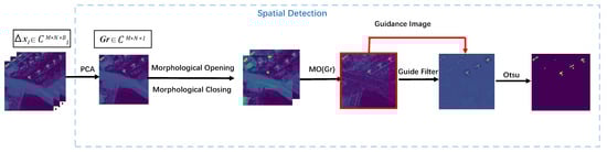
Figure 4.
The specific architecture of spatial detection.
Thirdly, to assist in removing false anomalous pixels from the , the guide filter [37] is used to dispose to get image :
where and are the average values of linear function coefficients covering all overlapping windows , respectively. itself is used as the guidance image. Relevant parameters in the guide filter are set according to the paper [30]. Finally, for making anomaly detection results more visual, the Otsu threshold algorithm [38] is applied to approximately process , converting them into a binary image of 0 and 1 to acquire the final spatial detection result.
3.2. Irredundant Pooling Regularized Mahalanobis Distance-Based Spectral Anomaly Detection
HSI contains abundant spectral and certain spatial features, where the former is vital to HAD. In our model, the IP regularized Mahalanobis distance-based spectral anomaly detection is put forward to extract spectral features better. It consists of IP, regularized Mahalanobis distance, and spectral detection. The IP is proposed to highlight the most useful HSI pixel component as much as possible by removing redundant information. Regularized Mahalanobis distance is used to calculate the distance between each pixel and background. Spectral detection is applied to process the distance matrix to obtain the final result in the spectral branch. The details are as follows.
3.2.1. Irredundant Pooling
HSI is usually composed of hundreds of bands but has the characteristics of information redundancy. Hence, spectral feature extraction of HAD would inevitably be interfered. To address the matter, the IP is appended. As illustrated in Figure 5, adjacent bands are divided into the same group.
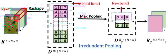
Figure 5.
The specific detail of Irredundant Pooling.
Then max pooling is applied to elements of each pixel vector in the group bands from spectral dimensionality. The max gray value is taken as the representative of the corresponding pixel in these bands. All pixels max gray value in this group form the new representative band. In this way, we can remove the redundant information while retaining the most useful pixel component, which plays a decisive role in solving the HSI redundant information disturbance issue.
3.2.2. Regularized Mahalanobis Distance
Mahalanobis distance is the most popular method in the field of AD, whose formula is:
where is the pixel vector corresponding to spatial position in the HSI, is the set of pixels in the whole HSI, represents the vector transpose, and u are the inverse of the covariance matrix and average vector of the , is on behalf of the Mahalanobis distance between the homologous pixel and background, and is the square root operation.
Unfortunately, the HSI covariance matrix may be ill-conditioned owing to high correlation dimensionality. As suggested by [39], the traditional Mahalanobis distance is modified. Under the premise that the energy of the matrix and correlation of the pixel vector element remains unchanged as far as possible, we add a bias matrix into the HSI covariance matrix, transforming it into a non-singular matrix. The altered formula is as follows:
where E is the identity matrix of the same order as and is the regularization coefficient.
The IP-based regularized Mahalanobis distance algorithm achieved the better performance. The distance matrix calculated by Equation (12) is the ultimate result of spectral branch anomaly detection.
3.3. Combination
There is rich spectral and certain spatial information in HSI. Thus, features extracted from spatial and spectral branch need to be merged to obtain complete information in the original HSI. The fusion is as follows:
where F is the final HAD result, and are the linear coefficients of spatial and spectral anomaly detection results, respectively. Considering that the two kinds of information are equally important in HSI, they are both fixed at 0.5.
4. Experiments
In this section, we introduce the four public HSI data sets [40], related algorithms used in comparative experiments, evaluation criteria, detection performance of different algorithms on these data sets, and parameters settings.
4.1. Data Description
- San Diego data set: It is taken by the Airborne Visible/Infrared Imaging Spectrometer (AVIRIS) from the San Diego area. They consist of 224 bands, however there are 35 bands of poor quality that are deleted in the experiment, such as water absorption region. Consequently, there are 189 bands in the effective data set and the spatial resolution is 3.5 m. The image size is , where areas from the upper left corners is selected for training and testing. Three aircraft are called anomalies, with a total of 57 anomalous pixels. The pseudo-color image and ground-truth map are shown in Figure 6a,b.
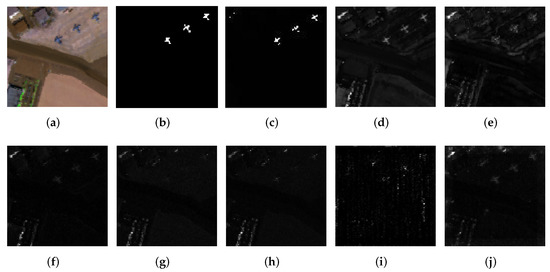 Figure 6. Visual detection results of all the algorithms on the San Diego dataset. (a) Pseudocolor image. (b) Ground-truth. (c) BEGAIP. (d) LRASR. (e) GTVLRR. (f) LSMAD. (g) RX. (h) RPCA. (i) LRX. (j) CRD.
 - Los Angeles data set: The region shown in this image acquired by AVIRIS is the part of urban area of Los Angeles. The spatial region size is , the spatial resolution is 7.1 m, and the number of available bands is 205. In the process of AD, ground objects of different shapes, such as aircraft are regarded as anomalies, with a total of 170 abnormal pixels. The pseudo-color and ground-truth image are demonstrated in Figure 7a,b.
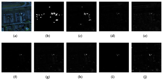 Figure 7. Visual detection results of all the algorithms on the Los Angeles dataset. (a) Pseudocolor image. (b) Ground-truth. (c) BEGAIP. (d) LRASR. (e) GTVLRR. (f) LSMAD. (g) RX. (h) RPCA. (i) LRX. (j) CRD.
 - Texas Coast data set (TC-I data set and TC-II data set): It includes some images taken by the AVIRIS in the Texas Coast Area. There are two images with a spatial size of , a spatial resolution of 17.2 m, and 207 available bands in total. Residential houses of different shapes in the image are labeled as anomalous areas, containing 67 and 155 anomalous pixels, respectively. Figure 8a,b describe the pseudo-color and the ground-truth map of TC-I. And Figure 9a,b show the pseudo-color and the ground-truth map of TC-II.
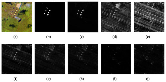 Figure 8. Visual detection results of all the algorithms on the TC-I dataset. (a) Pseudocolor image. (b) Ground-truth. (c) BEGAIP. (d) LRASR. (e) GTVLRR. (f) LSMAD. (g) RX. (h) RPCA. (i) LRX. (j) CRD.
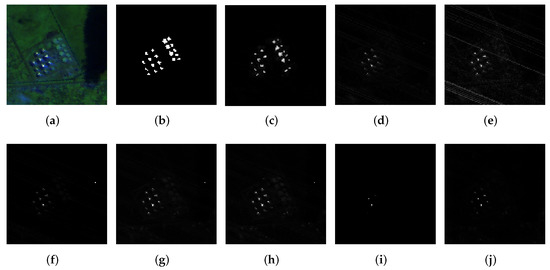 Figure 9. Visual detection results of all the algorithms on the TC-II dataset. (a) Pseudocolor image. (b) Ground-truth. (c) BEGAIP. (d) LRASR. (e) GTVLRR. (f) LSMAD. (g) RX. (h) RPCA. (i) LRX. (j) CRD.
 - Bay Champagne data set: It is collected by AVIRIS from the Bay Champagne area. The image is made up of 188 available bands, whose spatial size is and resolution is 4.4 m. Among them, things on the sea surface are considered as anomalies, involving 11 pixels. The pseudo-color and the real ground-truth of the image are given in Figure 10a,b.
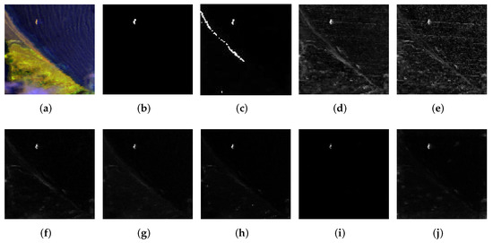 Figure 10. Visual detection results of all the algorithms on the Bay Champagne dataset. (a) Pseudocolor image. (b) Ground-truth. (c) BEGAIP. (d) LRASR. (e) GTVLRR. (f) LSMAD. (g) RX. (h) RPCA. (i) LRX. (j) CRD.
4.2. Compared Methods and Evaluation Criteria
In this part, the compared methods and evaluation criteria are introduced.
4.2.1. Compared Methods
Taking the theory adopted, influence, and popularity into consideration, classic AD algorithms in different time periods are selected. The compared algorithms cover RX [13], LRX [15], CRD [16], RPCA [41], GTVLRR [42], LRASR [17], and LSMAD [43].
The RX is the typical statistics-based algorithm, which supposes that the background obeys the standard normal distribution. Combined with mathematical knowledge, pixels’ Mahalanobis distance matrix is the criterion to judge whether a pixel is an anomaly. If the distance value is too large, the pixel is likely to be anomaly, otherwise, it belongs to the background. LRX is the variant of the RX, which is a little different from the RX. It deems that background in the local area obeys the standard normal distribution. As for CRD, a background pixel is approximately linearly expressed by the surroundings while the anomaly can not. The RPCA is another kind of representation-based algorithm, which decomposes HSI into two matrices: low-rank background and sparse anomaly matrix. Finally, the norm is imposed on the sparse matrix to detect an anomaly. For GTVLRR, the whole image pixels are chosen as the dictionary for simplicity. Aiming to take advantage of spatial information, the graph and total variation (TV) regularization are incorporated. Furthermore, the LRASR is the classic representation-based AD algorithm. It constructs the background dictionary used to linearly represent background pixels matrix by making use of clustering and then with the way of matrix decomposition, sparse matrix representing anomalies can be obtained. In addition, the sparse matrix is added to the norm for the final detection result. LSMAD is the representation-based version where the LRASR and Mahalanobis distance are combined to gain a better performance.
4.2.2. Evaluation Criteria
To compare the detection performance of the model proposed and other compared algorithms, the receiver operating characteristic (ROC) and the area under the curve (AUC) value are adopted as the evaluation criteria [44,45]. In the HAD evaluation area, ROC is the most popular [46]. It is like a function where the true positive rate () is uniquely determined when the false positive rate () is fixed. Besides, varies at the different threshold value. The and formula are as follows:
In fact, AD is an unsupervised pixel binary classification problem, including positive and negative class. In Equation (14), a positive pixel is predicted truly, which is denoted as . On the contrary, if a positive pixel is detected as a negative pixel falsely, it is denoted as . Similarly, in Equation (15), represents false positive rate and means the true negative rate. If and are independent variables and function values, respectively, then they can form a function picture. This function curve is called the ROC curve and its level indicates the performance of the tested model. In other words, the higher true positive rate () means better when the false positive rate () is the same. From a macro point of view, AUC (the area under ROC curve), is viewed as the evaluation criteria of relevant models and is less than 1.0.
4.3. Detection Performance
The experimental results conducted on four data sets are analyzed in this section. The AUC values on data sets of compared methods and BEGAIP model are described in Table 1.

Table 1.
AUC values of several methods on the four data sets.
Firstly, from the point of the AUC value, the detection performance analysis is as follows. As we can see, although the RX algorithm is seen as the benchmark, its detection effect on all data sets is relatively stable compared with other compared algorithms. In particular, its performance on the TC data set is only inferior to RPCA and the proposed algorithm’s. LRX achieved the best (0.9999) and second-best detection effect (0.9386) on the Bay Champagne and Los Angeles data set, respectively, however the worst detection result (0.8944) was on the San Diego data set. The overall performance is extremely unstable. Besides, it is greatly affected by the size of the window. If the size of the outer and inner windows are not appropriate, the result is extremely terrible. Comparatively speaking, the CRD algorithm has a stable performance. Besides, its AUC (0.9999) on the Bay Champagne data sets is the best. Low-rank and sparse representation-based algorithms, including GTVLRR, LRASR, and RPCA, fail to yield satisfying results. In contrast, LSMAD has a better comprehensive performance. The new model proposed had an excellent performance on four data sets. Its AUC values on the first three data sets are far higher than the second-ranked. However, it is not the best on the fourth data set, whose AUC value (0.9998) is only 0.0001 smaller than the LRX and CRD’s. This is because the compared algorithms do not make effective use of spatial features. Unlike them, the proposed model BEGAIP contains a branch based on BE and GAN to extract spatial features for HAD. Although BEGAIP achieves the best results on the Los Angeles data set compared to other algorithms, its AUC value is smaller than value obtained from other four HSIs. The reason is that the pixels that exist in the background and anomaly boundary area almost obey the Gaussian distribution. Therefore, these pixels are regarded as the background by two GANs. Besides, the anomaly area in this HSI data set is small. Hence, the reduction rate of the anomaly area detected by BEGAIP is greater than other data sets. However, the comprehensive results on the five HSI of BEGAIP are far better than the compared methods. In addition, the ROC curves are illustrated in Figure 11, which shows five HSIs in four data sets, respectively. As explained earlier, the higher the curve, the better corresponding algorithm performance. As the picture shows, in a, b, c, and d, the curves of BEGAIP are always above that of the compared algorithms. The BE and IP help to utilize spatial and spectral features better. As for e, the curve of model proposed is below others only when is small. The reason may be that the pixels at the shoreline location do not obey the Gaussian distribution and these pixels are mistakenly regarded as anomalies by BEGAIP. That leads to the matter that the false alarm rate of BEGAIP on the Bay Champagne data set is relatively higher than on other data sets. However, our model shows the best results when comparing the ROC curves in the five figures. It verifies the good performance of our model again.
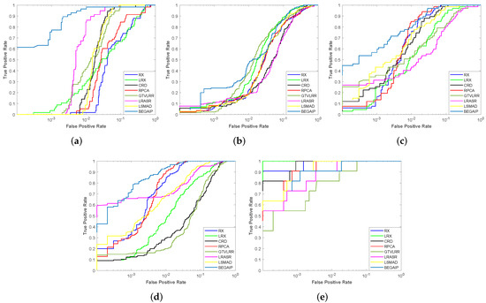
Figure 11.
ROC curves of all the algorithms on four data sets. (a) San Diego data set. (b) Los Angeles data set. (c) TC data set-I. (d) TC data set-II. (e) Bay Champagne data set.
Secondly, the visual detection results on data sets are portrayed in Figure 6, Figure 7, Figure 8, Figure 9 and Figure 10. They respectively correspond to the San Diego, Los Angeles, TC-I, TC-II, and Bay Champagne HSI data set, where a–j represent the true HSI, ground-truth, and detection result of different methods. From only the effect diagram of HAD, the BEGAIP’s performance is far better than that of the compared algorithms. In addition, it can be seen that the visual detection result texture structure of BEGAIP on five HSIs is clearer than the compared algorithms. The reason is that the BE-based spatial branch in our model takes spatial features into consideration, which brings about such a good result. In c of Figure 6 and Figure 8, Figure 9 and Figure 10, the anomaly area shape detected by BEGAIP is almost similar to the true anomaly area shape. Due to the anomaly area in these four HSI data sets being large, although some anomaly pixels in the boundary area between anomaly and background are not detected by the BEGAIP, the left area shape does not change too much. On the contrary, in c of Figure 7, some anomaly area is lost because these anomalies are almost boundary pixels obeying the Gaussian distribution. They are not detected by the model well. On the whole, from the view of the visual detection image and AUC value, a comprehensive performance of BEGAIP is shown to be better than the compared algorithms. BEGAIP is also suitable for the HSI data sets whose anomaly area is relatively large.
4.4. Parameters Settings
Relevant parameter settings are discussed in this part. The important parameters settings of all algorithms on the four data sets are portrayed in Table 2. As for BEGAIP, in the spatial branch, the of BE is set according to the experimental results shown in Figure 12, where is chosen from {1, 2, 3, 4, 5, 6, 7, 8}. As for the GAN network, they are set by experimental outcomes. The input dimension and output dimension of encoder En are and , which is equal to square roots of , consisting of 3 layers of a fully connected network followed by Leaky ReLu. The input and output dimension of Dz in the AE latent layer are and 1, which is composed of 3 layers of a fully connected network followed by Leaky ReLu and Dropout with a default parameter of 0.1. In the latent feature layer, , , and of the loss are 1, 0.1, and 0.05. In particular, the is a smooth loss with instead of the loss function. De and Do both compose of 3 layers of fully connected networks. The input and output dimension of the former are and while the latter are and 1. In the spatial detection, the guide filter size r and regularization parameter are 3 and 0.5 according to the works of [30].
Table 2.
Parameters Settings of algorithms on the data sets.
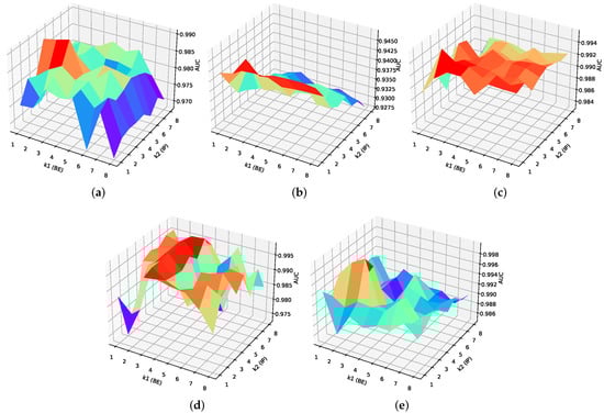
Figure 12.
The AUC value varies with parameters of K1 and K2. (a) San Diego data set. (b) Los Angeles data set. (c) TC data set-I. (d) TC data set-II. (e) Bay Champagne data set.
In the spectral branch, in accordance with many experimental results illustrated in Figure 12, in which varies in {1, 2, 3, 4, 5, 6, 7, 8}, the of IP is chosen for each data set. The bias matrix coefficient in (12) is fixed at 0.01, as recommended by [39]. Regarding the compared methods, there are no important parameters in RX and LSMAD. For LRX and CRD, their optimal outer and inner windows size are set on the basis of [47] and experiments, where the outer size varies from 5 to 29 and the inner size varies from 3 to 27. The suitable regularization parameter in CRD is set to , as suggested by the original literature [16]. Combining [17] and the experimental results, the perfect regularization parameter and of LRASR are selected from {} and {}, respectively, for each HSI. For GTVLRR, advised by [42], the suitable parameter , , and are picked from {}, {}, and {}, respectively for every data set. As to RPCA, the is fixed at in accordance with [48]. The relevant experiments were repeated 10 times, and the average value is taken as the final result.
Figure 12a–e shows that of BE and of the IP play an important part on the performance of model proposed. The variation curves of the BEGAIP performance with parameters or are similar to a parabola. As for the BE, the reason is that it discards some useful bands containing much background spatial features when is too large and its background spatial features enhancement degree is poor when is small, thus the GANs with a strong background generation ability can not be obtained. That accounts for the bad detection results. As for the IP, the new band generated by IP is meaningless because the pixel component dimension has no correlation when is too large and there is a large amount of redundant information when is small, which are both not beneficial to the subsequent spectral anomaly detection. Therefore, the parameters settings of and are vital to the performance of BEGAIP.
5. Investigations
In this section, in order to further verify the role of relevant components and the efficiency of the proposed model, some investigations are carried out and discussed from four perspectives. Firstly, three different version of IPs, including IP with min pooling, IP with average pooling, and IP with max pooling, are arranged to explore which pooling is the best for IP. Secondly, the role of innovative components, containing constrained functions, BE, and IP, is discussed according to the eight experimental scenarios’ results and adopted logic. Thirdly, the computing time of all the methods with the best parameters setting shown in Table 2 are recorded. Their computational efficiency is also evaluated by us. Finally, to confirm the robustness of our proposed model against noise, experiments are carried out on the HSI data set with synthetic noise.
5.1. Investigation of Different Version Irredundant Pooling (IP)
AUC values of IP with different pooling on the data sets are demonstrated in Table 3. The model without an IP and with the best parameters setting (BEGAIP without IP), which is the benchmark, are also conducted on the data sets to make the results persuasive.
Table 3.
AUC values of IP with different pooling on data sets.
From Table 3, we can see that the IP with min pooling obtains the worst results. Besides, BEGAIP without IP and IP with average pooling have a similar effect, as they did not consider the importance of features in adjacent bands at the same location of hyperspectral data, resulting in poor results. The version with IP (max pooling) is the most excellent among the experimental scenes. It ensures the best use of spectral features by highlighting the most significant components. Of course, group number , the number of the adjacent bands assigned to the same group, is also important. The process of the investigation is illustrated in Figure 12 and the results are recorded in Table 2, the optional parameter is from the {}.
5.2. Investigation of the Innovative Part
In this part, the innovations of our model are discussed from the view of the logic and application. The innovations include background spatial feature enhancement (BE), irredundant pooling (IP), and constrain function which is made up of , , and .
From the point of logic, the two GANs in the proposed model are used to learn the distribution law of the HSI pixels and to reconstruct the background image, the BE is aimed at enhancing the HSI spatial features. Thus, the BE-GANs would learn more background information to generate a more realistic background image. Although the GAN has a powerful data generation ability, it is not stable. The constrain function is imposed to prevent it from generating false background pixels. Of course, the constrain function can moderate, however not solve the instability problem of GANs thoroughly. The HSI has rich spectral features, however also information redundancy. IP is targeted at eliminating redundancy, while highlighting useful information, and protecting the spectral anomaly detection from being disturbed. By these analyses, we can learn that the innovations play a significant role to enhance the performance of BEGAIP for HAD.
To verify the role of the innovative part from the application view, a self-comparison experiment is conducted on the HSI data sets. Eight algorithm versions are prepared in total. We regard only two GANs without constrained functions loss in the spatial path and regularized Mahalanobis distance (MD) in the spectral branch as the benchmark, denoted as and arranged in the first experiment. The second is with additional reconstruction loss between the input of the GANz and output of the GANo, represented as . Similarly, the spectral angle constraint and latent layer constrain are added to the according to Figure 3. They are the third and fourth experimental scenarios, respectively. Three loss functions are imposed on the GAN networks together, which means the two GANs are constrained. It is assigned in the fifth, represented as . We add the BE to the spatial branch in the fifth scene. The view is of the and arranged in the sixth part. The IP is appended to the spectral branch in the fifth experiment, of which is the seventh scenario. The eighth corresponds to the BEGAIP proposed, comparing the fifth, sixth, and seventh experiment. It consists of BE and , denoted as . To avoid the experimental contingency, each experiment is repeated 5 times and the average AUC value is taken as the final result. The specific data are exhibited in Table 4.
Table 4.
AUC values of eight algorithm versions on the data sets.
As Table 4 shows, the benchmark algorithm obtains the worst results on five HSI datasets. The performance of the method of , , are better than the benchmark. This is because the proposed constrained functions ensure the GANs are stable. It can reconstruct the background image well. The AUC value of the fifth algorithm is far bigger than the benchmark. The reason is that when these three constrained functions are combined, the two GANs networks become more stable. Thus, the GANs can better reconstruct the background image. The result of the is better than the fifth method. This is because the BE can provide HSI with background spatial features enhanced for constrained two GANs training. Therefore, the first GAN (GANz) would generate a low dimensional background image with more pure background spatial features, which is beneficial for the second GAN (GANo) to reconstruct the background image. The AUC value of the seventh method is bigger than the fifth method. IP, removing the redundant information and highlighting the most useful information, prevents spectral anomaly detection from redundant information interference. Thus, the seventh method obtains a better result when compared to the fifth algorithm. Therefore, the results in Table 4 verify the positive effect of the innovative part, including the constrained function, BE, and IP again.
5.3. Investigation of Computing Time
The experiments of model BEGAIP were conducted on GeForce RTX 2070 SUPER, Pycharm 2019.3.3 x64, Python 3.6.0, torch-gpu 1.8.1, and CUDA 11.1.96. We used MATLAB R2020a for the experiments of the compared methods on GeForce RTX 2070 SUPER. The time cost of all the algorithms on the data sets is demonstrated in Table 5 and the processing time of BEGAIP proposed, varying with the HSI spatial size and spectral dimensions is illustrated in Figure 13, which are recorded in seconds.
Table 5.
Average time cost (second) of all the algorithms on the data sets.
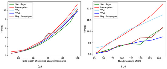
Figure 13.
The processing time of the proposed BEGAIP varies with the HSI spatial size and spectral dimensions. (a) The processing time varies with the spatial size when the spectral dimensions are fixed. (b) The processing time varies with the spectral dimension when the spatial size is fixed.
The network proposed is complex owing to many parameters that need to be learned in the spatial branch. It may spend twenty minutes optimizing and training. In this article, the time from the data input to acquisition of detection result, excluding GAN training time, is taken as the computing time. As displayed in Table 5, it can be concluded that BEGAIP is not the best algorithm, however it is quicker than LRX, GTVLRR, LRASR, LSMAD except RX, CRD, and RPCA. Although the application of GANs has improved the accuracy, they result in the expense of time. How to reduce computing time would be a concern for future work. Nevertheless, the comprehensive result, involving the AUC value and visual detection image, is far better than that of RX, CRD, and RPCA. It again confirms the performance of the method designed for HAD.
In order to explore how the processing time increases with respect to the size of the image, two groups of experiments are conducted on HIS data sets. In the first group of experiments, the dimensions of four HIS data sets are fixed, and we change the spatial size of the selected square HSI area for the experiments. Each time, we add 10 to the side length of the region. In this way, we can learn how the processing time varies with an increase in spatial size. In the second group of experiments, the spatial size is fixed at 100×100, and we add the 30 bands every time to explore how the processing time increases with respect to the dimensions of the image. The results are shown in Figure 13:
In the picture, we can see that the spatial size and spectral dimensions of the HSI have an important effect on the processing time of the model. In Figure 13a,b, the computing time becomes bigger along with an enlarged spatial size or increased spectral dimensions. The reason being that the number of parameters that need to be learned increases in spatial branch and the scale of matrix processed enlarges in the spectral branch. When spatial sizes or channels of different HSI are the same, the processing time is different. This is because the grouping band selection in BE and redundant information elimination of IP change dimensions of HSI to be processed.
5.4. Investigation of Model BEGAIP for HAD Robustness against Noise
In this section, we confirm the robustness of BEGAIP against noise when it is used for HAD. Firstly, Gaussian noises with a different signal-to-noise ratio (SNR) {10 dB, 20 dB, 30 dB, 40 dB, 50 dB, 60 dB, 70 dB, 80 dB} are added to four HSI data sets. The mean and standard deviation of noise are 0 and 1, respectively. Then, several experiments are conducted on these synthetic data sets. The results are shown in Figure 14.
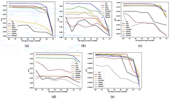
Figure 14.
ROC curves of all the algorithms on four synthetic data sets. (a) San Diego data set. (b) Los Angeles data set. (c) TC data set-I. (d) TC data set-II. (e) Bay Champagne data set.
As we can see, the robustness of BEGAIP against noise is not the best, however it is excellent when it is used for HAD. In Figure 14, the ROC curves of model proposed in a, c, d, and e are stable when SNR is bigger than 30 dB, and decline when SNR is smaller than 30 dB. Since the , constrained two GANs, and Mahalanobis distance can eliminate the influence of a small amount of noise on HAD. Besides, the anomaly area in these three HSIs is relatively large, and the energy of the background in each band has a bigger discrimination degree. Therefore, the BE can obtain a more pure background spatial feature set. The constrained two GANs can reconstruct the background image well. However, when SNR is lower than 30 dB, there is considerable noise in these three data sets and HSIs are almost damaged. For , constrained two GANs and Mahalanobis distance can not completely eliminate the noise effect on HAD, which leads to bad results. The BEGAIP curve of b slightly fluctuates when the SNR is higher than 30 dB, which is due to the smaller anomaly area in the synthetic HSI data. On the whole, the proposed model has good robustness to noise when it is used for HAD.
6. Conclusions
In this article, a new model called BEGAIP is designed for HAD. The BE is applied to acquire a relatively pure background spatial information data set for the GAN networks training, strong constrain functions make GAN network stable and IP is made use of to remove redundant information. The method is examined on four HSI data sets and the experimental results show that our model is better than the relevant classical algorithms based on RX and low-rank sparse representation. From the perspective of the AUC value, the proposed BEGAIP is excellent. From the view of the visual detection image, the anomaly in the HSI can be recognized easily through different colors. Besides, the computing time of the proposed model on the HSI data sets is less than that of the LRX, GTVLRR, LRASR, and LSMAD algorithms.
From the reflection of the experimental process, we have learnt some lessons. As for the model collapse owing to the unstability of GAN, selecting the ideal epoch and designing strong constrained functions are good choices. The learning rate of the optimizer is also significant to the performance of the model.
Of course, the false alarm rate is relatively high in the final detection map on a certain data set, where there are some pixels included in the background, however are mistaken as anomalies. In future, some time needs to be spent designing more efficient networks, reducing the false alarm rate, and processing anomalies in the boundary area well to further enhance its performance.
Author Contributions
Conceptualization, Z.L. and S.S.; methodology, Z.L., S.S., M.X. and L.W.; software, Z.L., S.S., L.W. and L.L.; validation, Z.L., M.X. and L.L.; writing—original draft preparation, M.X. and S.S.; writing—review and editing, Z.L., L.W. and L.L.; project administration, Z.L. and M.X.; funding acquisition, Z.L. and L.W. All authors read and agreed to the published version of the manuscript.
Funding
This research was funded by the Joint Funds of the National Natural Science Foundation of China, Grant Number U1906217, the General Program of the National Natural Science Foundation of China, Grant Number 62071491, and the Fundamental Research Funds for the Central Universities, Grant No. 19CX05003A-11.
Acknowledgments
The author is grateful to their teachers for his advice when designing the model and the technology support when doing the experiment, and thanks is also given to their classmates and teachers for their help in polishing and typesetting the articles. These works have played a positive role in completing this article.
Conflicts of Interest
The authors declare no conflict of interest. The funders had no role in the design of the study; in the collection, analyses, or interpretation of data; in the writing of the manuscript; nor in the decision to publish the results.
References
- Bioucas-Dias, J.M.; Plaza, A.; Camps-Valls, G.; Scheunders, P.; Nasrabadi, N.; Chanussot, J. Hyperspectral remote sensing data analysis and future challenges. IEEE Geosci. Remote Sens. Mag. 2013, 1, 6–36. [Google Scholar] [CrossRef] [Green Version]
- Guo, F.; Li, Z.; Xin, Z.; Zhu, X.; Wang, L.; Zhang, J. Dual Graph U-Nets for Hyperspectral Image Classification. IEEE J. Sel. Top. Appl. Earth Obs. Remote Sens. 2021, 14, 8160–8170. [Google Scholar] [CrossRef]
- Zhang, L.; Zhang, L.; Du, B.; You, J.; Tao, D. Hyperspectral image unsupervised classification by robust manifold matrix factorization. Inf. Sci. 2019, 485, 154–169. [Google Scholar] [CrossRef]
- Li, Z.; Cui, X.; Wang, L.; Zhang, H.; Zhu, X.; Zhang, Y. Spectral and Spatial Global Context Attention for Hyperspectral Image Classification. Remote Sens. 2021, 13, 771. [Google Scholar] [CrossRef]
- Zhang, X.; Li, C.; Zhang, J.; Chen, Q.; Feng, J.; Jiao, L.; Zhou, H. Hyperspectral unmixing via low-rank representation with space consistency constraint and spectral library pruning. Remote Sens. 2018, 10, 339. [Google Scholar] [CrossRef] [Green Version]
- Nasrabadi, N.M. Hyperspectral target detection: An overview of current and future challenges. IEEE Signal Process. Mag. 2013, 31, 34–44. [Google Scholar] [CrossRef]
- Zhong, Y.; Wang, X.; Xu, Y.; Wang, S.; Jia, T.; Hu, X.; Zhao, J.; Wei, L.; Zhang, L. Mini-UAV-borne hyperspectral remote sensing: From observation and processing to applications. IEEE Geosci. Remote Sens. Mag. 2018, 6, 46–62. [Google Scholar] [CrossRef]
- Xie, W.; Zhang, X.; Li, Y.; Wang, K.; Du, Q. Background learning based on target suppression constraint for hyperspectral target detection. IEEE J. Sel. Top. Appl. Earth Obs. Remote Sens. 2020, 13, 5887–5897. [Google Scholar] [CrossRef]
- Zhang, Y.; Wu, K.; Du, B.; Hu, X. Multitask learning-based reliability analysis for hyperspectral target detection. IEEE J. Sel. Top. Appl. Earth Obs. Remote Sens. 2019, 12, 2135–2147. [Google Scholar] [CrossRef]
- Li, L.; Li, W.; Du, Q.; Tao, R. Low-rank and sparse decomposition with mixture of gaussian for hyperspectral anomaly detection. IEEE Trans. Cybern. 2020, 51, 4363–4372. [Google Scholar] [CrossRef]
- Su, H.; Wu, Z.; Zhu, A.; Du, Q. Low rank and collaborative representation for hyperspectral anomaly detection via robust dictionary construction. ISPRS J. Photogramm. Remote Sens. 2020, 169, 195–211. [Google Scholar] [CrossRef]
- Zhao, G.; Li, F.; Zhang, X.; Laakso, K.; Chan, J.C.W. Archetypal Analysis and Structured Sparse Representation for Hyperspectral Anomaly Detection. Remote Sens. 2021, 13, 4102. [Google Scholar] [CrossRef]
- Reed, I.S.; Yu, X. Adaptive multiple-band CFAR detection of an optical pattern with unknown spectral distribution. IEEE Trans. Signal Process. 1990, 38, 1760–1770. [Google Scholar] [CrossRef]
- Goldberg, H.; Kwon, H.; Nasrabadi, N.M. Kernel eigenspace separation transform for subspace anomaly detection in hyperspectral imagery. IEEE Geosci. Remote Sens. Lett. 2007, 4, 581–585. [Google Scholar] [CrossRef]
- Molero, J.M.; Garzon, E.M.; Garcia, I.; Plaza, A. Analysis and optimizations of global and local versions of the RX algorithm for anomaly detection in hyperspectral data. IEEE J. Sel. Top. Appl. Earth Obs. Remote Sens. 2013, 6, 801–814. [Google Scholar] [CrossRef]
- Li, W.; Du, Q. Collaborative representation for hyperspectral anomaly detection. IEEE Trans. Geosci. Remote Sens. 2014, 53, 1463–1474. [Google Scholar] [CrossRef]
- Xu, Y.; Wu, Z.; Li, J.; Plaza, A.; Wei, Z. Anomaly detection in hyperspectral images based on low-rank and sparse representation. IEEE Trans. Geosci. Remote Sens. 2015, 54, 1990–2000. [Google Scholar] [CrossRef]
- Huyan, N.; Zhang, X.; Zhou, H.; Jiao, L. Hyperspectral anomaly detection via background and potential anomaly dictionaries construction. IEEE Trans. Geosci. Remote Sens. 2018, 57, 2263–2276. [Google Scholar] [CrossRef] [Green Version]
- Alhashim, I.; Wonka, P. High quality monocular depth estimation via transfer learning. arXiv 2018, arXiv:1812.11941. [Google Scholar]
- Demertzis, K.; Iliadis, L. GeoAI: A model-agnostic meta-ensemble zero-shot learning method for hyperspectral image analysis and classification. Algorithms 2020, 13, 61. [Google Scholar] [CrossRef] [Green Version]
- Kendall, A.; Gal, Y.; Cipolla, R. Multi-task learning using uncertainty to weigh losses for scene geometry and semantics. In Proceedings of the IEEE Conference on Computer Vision and Pattern Recognition (CVPR), Salt Lake City, UT, USA, 18–22 June 2018; pp. 7482–7491. [Google Scholar]
- Lei, J.; Xie, W.; Yang, J.; Li, Y.; Chang, C.I. Spectral–spatial feature extraction for hyperspectral anomaly detection. IEEE Trans. Geosci. Remote Sens. 2019, 57, 8131–8143. [Google Scholar] [CrossRef]
- Chalapathy, R.; Chawla, S. Deep learning for anomaly detection: A survey. arXiv 2019, arXiv:1901.03407. [Google Scholar]
- Azarang, A.; Manoochehri, H.E.; Kehtarnavaz, N. Convolutional autoencoder-based multispectral image fusion. IEEE Access 2019, 7, 35673–35683. [Google Scholar] [CrossRef]
- Jiang, T.; Li, Y.; Xie, W.; Du, Q. Discriminative reconstruction constrained generative adversarial network for hyperspectral anomaly detection. IEEE Trans. Geosci. Remote Sens. 2020, 58, 4666–4679. [Google Scholar] [CrossRef]
- Xie, W.; Liu, B.; Li, Y.; Lei, J.; Du, Q. Autoencoder and adversarial-learning-based semisupervised background estimation for hyperspectral anomaly detection. IEEE Trans. Geosci. Remote Sens. 2020, 58, 5416–5427. [Google Scholar] [CrossRef]
- Goodfellow, I.; Pouget-Abadie, J.; Mirza, M.; Xu, B.; Warde-Farley, D.; Ozair, S.; Courville, A.; Bengio, Y. Generative adversarial nets. Adv. Neural Inf. Process. Syst. 2014, 27, 2672–2680. [Google Scholar]
- Chao, X.; Cao, J.; Lu, Y.; Dai, Q.; Liang, S. Constrained Generative Adversarial Networks. IEEE Access 2021, 9, 19208–19218. [Google Scholar] [CrossRef]
- Lopez-Martin, M.; Sanchez-Esguevillas, A.; Arribas, J.I.; Carro, B. Supervised contrastive learning over prototype-label embeddings for network intrusion detection. Inf. Fusion 2022, 79, 200–228. [Google Scholar] [CrossRef]
- Xie, W.; Jiang, T.; Li, Y.; Jia, X.; Lei, J. Structure tensor and guided filtering-based algorithm for hyperspectral anomaly detection. IEEE Trans. Geosci. Remote Sens. 2019, 57, 4218–4230. [Google Scholar] [CrossRef]
- Wold, S.; Esbensen, K.; Geladi, P. Principal component analysis. Chemom. Intell. Lab. Syst. 1987, 2, 37–52. [Google Scholar] [CrossRef]
- LeCun, Y.; Bottou, L.; Bengio, Y.; Haffner, P. Gradient-based learning applied to document recognition. Proc. IEEE. 1998, 86, 2278–2324. [Google Scholar] [CrossRef] [Green Version]
- Choi, J.; Han, B. MCL-GAN: Generative Adversarial Networks with Multiple Specialized Discriminators. arXiv 2021, arXiv:2107.07260. [Google Scholar]
- Lopez-Martin, M.; Carro, B.; Sanchez-Esguevillas, A. Variational data generative model for intrusion detection. Knowl. Inf. Syst. 2019, 60, 569–590. [Google Scholar] [CrossRef]
- Mao, X.; Li, Q.; Xie, H.; Lau, R.Y.; Wang, Z.; Paul Smolley, S. Least squares generative adversarial networks. In Proceedings of the IEEE International Conference on Computer Vision (ICCV), Venice, Italy, 22–29 October 2017; pp. 2794–2802. [Google Scholar]
- Parhi, R.; Nowak, R.D. The role of neural network activation functions. IEEE Signal Process. Lett. 2020, 27, 1779–1783. [Google Scholar] [CrossRef]
- He, K.; Sun, J.; Tang, X. Guided image filtering. IEEE Trans. Pattern Anal. Mach. Intell. 2012, 35, 1397–1409. [Google Scholar] [CrossRef]
- Eldeeb, H.H.; Zhao, H.; Mohammed, O.A. Detection of TTF in Induction Motor Vector Drives for EV Applications via Ostu’s-Based DDWE. IEEE Trans. Transp. Electrif. 2020, 7, 114–132. [Google Scholar] [CrossRef]
- Xu, Y.; Wu, Z.; Chanussot, J.; Wei, Z. Joint reconstruction and anomaly detection from compressive hyperspectral images using Mahalanobis distance-regularized tensor RPCA. IEEE Trans. Geosci. Remote Sens. 2018, 56, 2919–2930. [Google Scholar] [CrossRef]
- Kang, X.; Zhang, X.; Li, S.; Li, K.; Li, J.; Benediktsson, J.A. Hyperspectral anomaly detection with attribute and edge-preserving filters. IEEE Trans. Geosci. Remote Sens. 2017, 55, 5600–5611. [Google Scholar] [CrossRef]
- Chen, S.Y.; Yang, S.; Kalpakis, K.; Chang, C.I. Low-rank decomposition-based anomaly detection. In Proceedings of the Algorithms and Technologies for Multispectral, Hyperspectral, and Ultraspectral Imagery XIX, Baltimore, MD, USA, 18 May 2013; p. 87430N. [Google Scholar]
- Cheng, T.; Wang, B. Graph and total variation regularized low-rank representation for hyperspectral anomaly detection. IEEE Trans. Geosci. Remote Sens. 2019, 58, 391–406. [Google Scholar] [CrossRef]
- Zhang, Y.; Du, B.; Zhang, L.; Wang, S. A low-rank and sparse matrix decomposition-based Mahalanobis distance method for hyperspectral anomaly detection. IEEE Trans. Geosci. Remote Sens. 2015, 54, 1376–1389. [Google Scholar] [CrossRef]
- Tan, K.; Hou, Z.; Ma, D.; Chen, Y.; Du, Q. Anomaly detection in hyperspectral imagery based on low-rank representation incorporating a spatial constraint. Remote Sens. 2019, 11, 1578. [Google Scholar] [CrossRef] [Green Version]
- Chang, S.; Du, B.; Zhang, L. BASO: A background-anomaly component projection and separation optimized filter for anomaly detection in hyperspectral images. IEEE Trans. Geosci. Remote Sens. 2018, 56, 3747–3761. [Google Scholar] [CrossRef]
- Xiang, P.; Song, J.; Li, H.; Gu, L.; Zhou, H. Hyperspectral anomaly detection with harmonic analysis and low-rank decomposition. Remote Sens. 2019, 11, 3028. [Google Scholar] [CrossRef] [Green Version]
- Xie, W.; Li, Y.; Lei, J.; Yang, J.; Chang, C.I.; Li, Z. Hyperspectral band selection for spectral–spatial anomaly detection. IEEE Trans. Geosci. Remote Sens. 2019, 58, 3426–3436. [Google Scholar] [CrossRef]
- Ma, X.; Zhang, X.; Tang, X.; Zhou, H.; Jiao, L. Hyperspectral anomaly detection based on low-rank representation with data-driven projection and dictionary construction. IEEE J. Sel. Top. Appl. Earth Obs. Remote Sens. 2020, 13, 2226–2239. [Google Scholar] [CrossRef]
Publisher’s Note: MDPI stays neutral with regard to jurisdictional claims in published maps and institutional affiliations. |
© 2022 by the authors. Licensee MDPI, Basel, Switzerland. This article is an open access article distributed under the terms and conditions of the Creative Commons Attribution (CC BY) license (https://creativecommons.org/licenses/by/4.0/).