Blind Remote Sensing Image Deblurring Using Local Binary Pattern Prior

Abstract

In this paper, an algorithm based on local binary pattern (LBP) is proposed to obtain clear remote sensing images under the premise of unknown causes of blurring. We find that LBP can completely record the texture features of the images, which will not change widely due to the generation of blur. Therefore, LBP prior is proposed, which can filter out the pixels containing important textures in the blurry image through the mapping relationship. The corresponding processing methods are adopted for different types of pixels to cope with the challenges brought by the rich texture and details of remote sensing images and prevent over-sharpening. However, the existence of LBP prior increases the difficulty of solving the model. To solve the model, we construct the projected alternating minimization (PAM) algorithm that involves the construction of the mapping matrix, the fast iterative shrinkage-thresholding algorithm (FISTA) and the half-quadratic splitting method. Experiments with the AID dataset show that the proposed method can achieve highly competitive processing results for remote sensing images.

1. Introduction

Affected by many factors, such as the imaging environment and camera shake, an acquired image may face the problems of image quality degradation and loss of important details caused by blurring during the imaging process. Therefore, it is necessary to study how to restore the image without prior knowledge, i.e., blind image deblurring. Ideally, the image quality degradation model can be expressed as:

$$G=H\ast U+N$$

(1)

where G, H, U, and N represent the blurry image, the blur kernel, original clear image, and noise, respectively. * represents convolution operator. Obviously, this is a typical ill-posed problem with countless conditional solutions. In order to find the optimal solution, we need to use the image feature information to change an ill-posed equation into a benign equation. Traditional image deblurring algorithms are generally divided into two parts: blind image deblurring algorithm, which can estimate an accurate blur kernel, and non-blind image deblurring that uses the estimated blur kernel to obtain a clear image.

Early image restoration algorithms used parameterized models to estimate blur kernels [1,2]. Still, the real blur kernels rarely follow the parameterized models, which leads to the lack of universality of such methods. After the total variation model proposed by Rudin et al. [3] in 1992, the theory of partial differential equations has become more and more popular in blind image restoration algorithms. Since then, researchers have designed two algorithmic frameworks based on theories of probability and statistics: Maximum a posteriori (MAP) [4,5,6,7] and Variational Bayes (VB) [8,9,10,11,12]. Although VB-based algorithms have good stability, their rapid development is permanently restricted by the complexity and vast calculation. On the contrary, MAP-based methods are relatively simple. However, Levin et al. [13] pointed out that the naive MAP approach, which is based on the sparse derivative prior, cannot achieve the expected effect. Therefore, it is necessary to introduce an appropriate blur kernel prior and delay the blur kernel normalization. Analyzing probability, the issue is recovering the clear image U and the blur kernel H simultaneously. This is equivalent to solving the standard maximum posterior probability. It can be expressed as:

$$(U,H)=argmaxP(U,H|G)\propto argmaxP(G|U,H)P\left(U\right)P\left(H\right)$$

(2)

where $P\left(G\right|U,H)$ is the noise distribution; $P\left(U\right)$ and $P\left(H\right)$ are the prior distributions of the latent clear image and blur kernel, respectively. After taking the negative logarithm of each item in (2), it is equivalent to the following regular model:

$$(U,H)=argmin\psi (G-H\ast U)+{\alpha }_{}\Phi \left(U\right)+{\beta }_{}\Psi \left(H\right)$$

(3)

where $\psi (:)$ is the fidelity term, $\Phi \left(U\right)$ and $\Phi \left(H\right)$ are regularization functions about U and H. $\alpha$ and $\beta$ are the corresponding parameters.

Under the MAP framework, some algorithms seek the optimal solution by utilizing sharp edges. However, when sharp edges are missing in some images, solving the problem requires prior knowledge that can distinguish between clear images and blurry images. Pan et al. [14] noted the difference in dark channel pixel distribution between the clear and blurry images. They proposed the dark channel prior, which performed well in processing natural, text, facial, and low-light images. To avoid the algorithm failure caused by insufficient dark channel pixels in the image, Yan et al. [15] introduced both dark channels and bright channels into the image-blind deblurring model. Ge et al. [16] pointed out that the above two methods will fail when there are insufficient extreme pixels. Therefore, they constructed a non-linear channel (NLC) prior and introduced it into a blind images deblurring algorithm. However, these methods may not perform well in processing remote sensing images.

In this paper, we notice that the similarity of LBP for clear and blurry images can be applied to blind image deblurring. A new optimization algorithm is proposed, inspired by algorithms based on extreme channels and local priors. We use the local binary pattern (LBP) [17] as the threshold to filter critical pixels containing texture features by establishing their mapping relationship to the image, the intensities of which will be accumulated by the strong convex $L_1$-norm. The gradients of different types of pixels will be processed correspondingly using the $L_0$-norm and $L_2$-norm. It is complicated to solve the restoration model directly, so the original problem needs to be decomposed into multiple sub-problems using the half-quadratic splitting method to facilitate results. In addition, we indirectly optimize the LBP prior by constructing a linear operator and adopt fast iterative shrinkage-thresholding algorithm (FISTA) [18] to solve the related equations. The contributions of this paper are as follows:

(1)

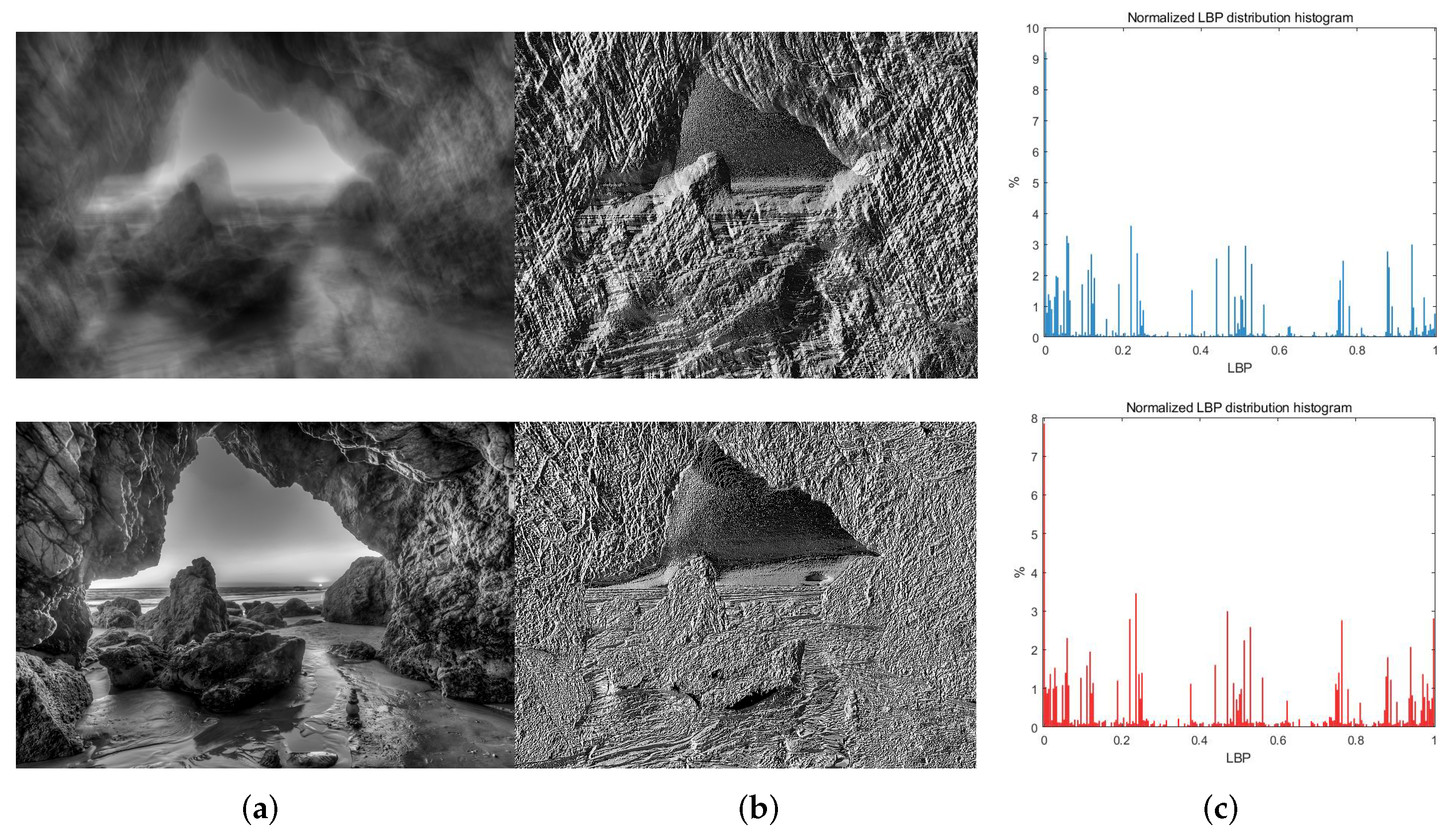
We note that LBP can completely extract the texture features of the images, which will not change significantly due to the presence of blur. Therefore, the LBP of the image can be used to locate the pixels that contain important texture information in the image by mapping.

(2)

A new remote sensing image deblurring algorithm based on LBP prior is proposed, which can remove the blur in the image and prevent over-sharpening by classifying all pixels and processing them in different ways.

(3)

As shown in the results, our proposed method, which has good stability and convergence, achieves extremely competitive results for remote sensing images.

The outline of the paper is as follows: Section 2 summarizes the related work in the field of image deblurring in recent years. Section 3 introduces the LBP prior and establishes the image-blind deblurring model and the corresponding optimization algorithm. Section 4 is the display of algorithm processing results. Section 5 makes a quantitative analysis of the performance of the proposed algorithm and discusses our algorithm after sufficient analysis and obtaining experimental results. Section 6 is the conclusion of this article.

2. Related Work

Blind image deblurring is now roughly divided into three categories: edge selection-based algorithms, image prior knowledge-based algorithms and deep learning-based algorithms. This part summarizes the achievements of blind image restoration in recent years.

2.1. Edge Selection-Based Algorithms

As one of the key features of recorded image information, edge information is widely used in image deblurring. Joshi et al. [19] used sub-pixel differences to locate important edges to estimate the blur kernel. Cho and Lee [20] proposed bilateral filters and impulsed filters to extract edge information in images. Xu and Jia [21] found that when the size of the edge is smaller than the blur kernel’s, it will affect the estimation of the kernel. Therefore, they proposed a new two-stage processing scheme based on the edge selection criteria. Sun et al. [22] used a patch method to extract edge information. However, this algorithm has a lot of calculation and time-consuming image processing. When there are insufficient sharp edges in an image, edge selection-based algorithms will fail. However, in the algorithms based on prior knowledge, the image edge information does not disappear, which is hidden in the regular term or prior knowledge, i.e., the low-rank characteristics of the gradient [23], $L_0$-norm of the gradient of the latent image [24] and the local maximum gradient prior [25], etc. In the restoration of hyperspectral images, gradient information has also received much attention. Yuzuriha et al. [26] took into account the low-rank nature of the gradient domain into the restoration model to make it better able to deal with anomalous variations.

2.2. Image Priors-Based Algorithms

Observing the clear and blurry images, much prior conducive to image restoration is applied to the algorithm. Shan et al. [27] used a probability model to process natural images with noise and blur. Krishnan et al. [28] proposed the $L_1$/$L_2$ norm with sparse features after analyzing the statistical characteristics of the image. Levin et al. [10] designed the maximum a posterior (MAP) framework based on the characteristics of image pixel distribution. Kotera et al. [29] improved the MAP method using image priors, which are heavier tail than Laplace, and applied a method of augmented Lagrangian. Michaeli and Irani [30] used the recursive characteristics of image patches at different scales to restore images. Ren et al. [23] adopted a method of minimizing the weighted nuclear norm, which combined the low rank prior of similar patches the blurry image and its gradient map, to enhance the effectiveness of the image deblurring algorithm. Zhong et al. [31] proposed a high-order variational model to process blurred images with impulse noise. After Pan et al. [14] used a dark channel prior for image deblurring and achieved excellent results, the sparse channel has attracted much attention in blind image deblurring. Yan et al. [15] combined dark channel and bright channel and designed an extreme channel prior algorithm. Since then, Yang [32] and Ge [16] have made further improvements to the problems faced by the extreme channel prior algorithms. At the same time, the blind image deblurring algorithms, based on local prior information, have also made significant achievements, i.e., the method based on the local maximum gradient (LMG) prior proposed by Chen et al. [25] and the method based on the local maximum difference (LMD) prior proposed by Liu et al. [33]. The algorithm we proposed also belongs to this category. Recently, Zhou et al. [34] established the image deblurring model of the luminance channel in YCrCb colorspace based on the dark channel prior, which expands a new idea for better processing color images. The image deblurring algorithm proposed by Chen et al. [35], which takes advantage of both saturated and unsaturated pixels in the image, effectively removes the blur of night scene images and has excellent inspiration for the processing of night remote sensing images.The restoration of hyperspectral images generally uses low-rank priors [26,36,37].

2.3. Deep Learning-Based Deblurring Methods

With the development of deep learning technology, related image deblurring algorithms have also been developed. Early learning networks, such as those proposed by Sun et al. [38] and Schuler et al. [39], were still designed based on the alternating directions method of multipliers used in traditional algorithms. Li et al. [40] combined deep learning networks with traditional algorithms, which use neural network learning priors to distinguish images. However, it is inferior when dealing with some complex and severely motion-blurred images. Some methods do not need to estimate the blur kernel, which can obtain clear images directly through training. For example, Nah et al. [41] trained a multi-scale convolutional neural network (CNN). Cai et al. [42] introduced the extreme channel prior to CNN. Zhang et al. [43] and Suin et al. [44] use multi-patch networks to improve performance. In order to reduce the computational complexity of the algorithm and obtain sufficient image information, the feature pyramid has become the focus of multi-scale learning. Lin et al. [45] proposed a feature pyramid network (FPN) that can fuse mapping information of different resolutions. In the field of deep learning, new networks are constantly being proposed to deal with different imaging situations and take shorter processing time, i.e., GAMSNet [46], ID-Net [47], DCTResNet [48] and LSFNet [49]. However, these methods have many model parameters and require a large number of data sets for long-term training to achieve good processing results.

3. Local Binary Pattern Prior Model and Optimization

In this part, we briefly introduced the local prior, i.e., LBP, and constructed an optimization model based on the LBP prior for blind image deblurring.

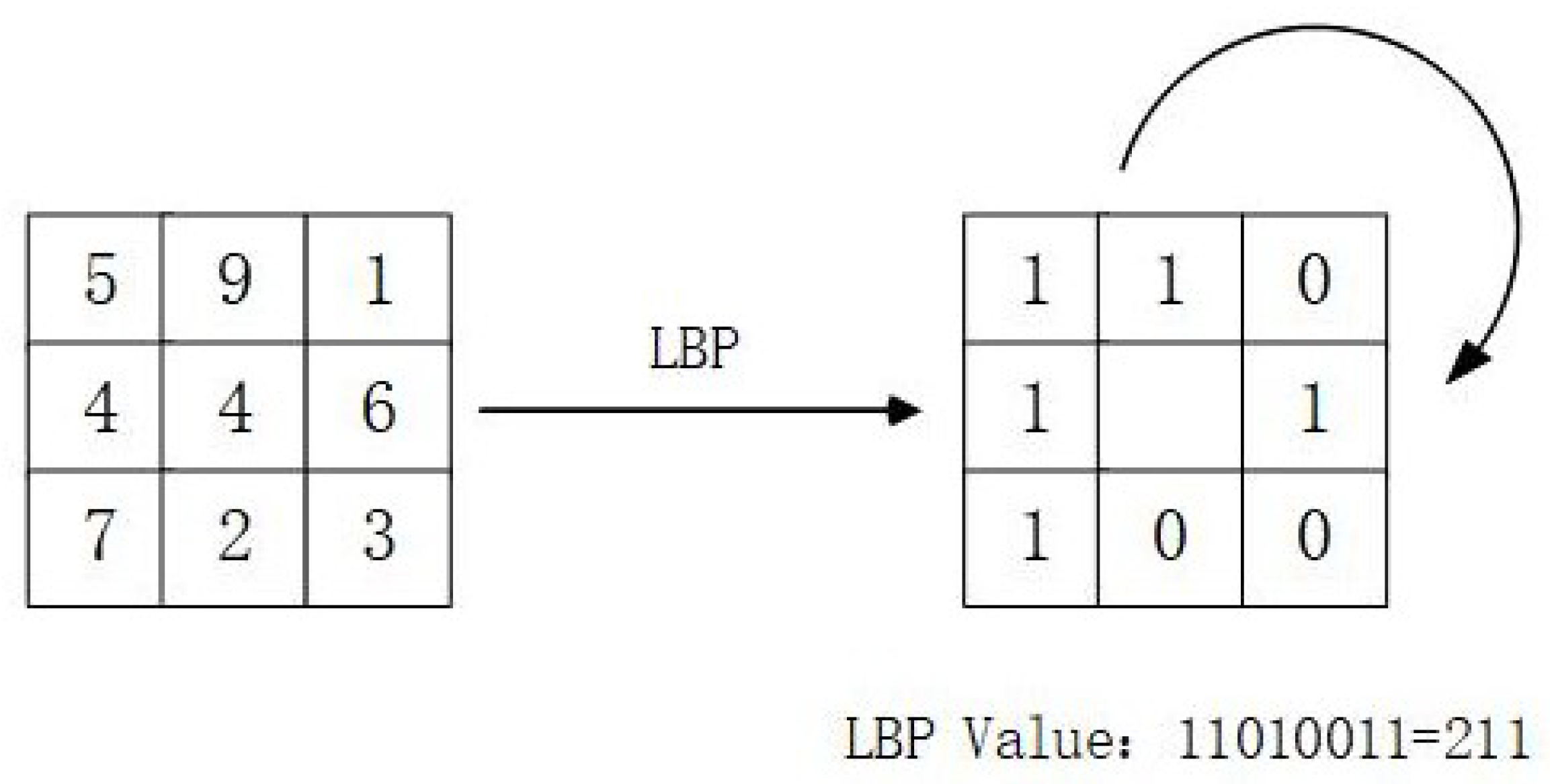
3.1. The Local Binary Pattern

LBP, the characteristics of intensity and rotation invariance, can extract local texture features in an image. Its principle is shown in Figure 1. In a window with the size of 3 × 3, the center pixel is compared with its 8-neighbor pixels. When a peripheral pixel is smaller than the center pixel, the location of the peripheral pixel is marked as 0; otherwise, it is recorded as 1. After that, we encode the 8-bit binary number generated to obtain the LBP value corresponding to the center pixel of the window.

Its formula is expressed as:

$$\mathrm{LBP}({\mathrm{a}}_c,b_c)=\sum _{p=0}^7{2}^{p}s(g_p-g_c)$$

(4)

where $({\mathrm{a}}_c,b_c)$ is the center pixel, $g_c$ is the intensity of the central pixel, $g_p$ is the intensity of the peripheral pixel, s(t) is the sign function.

$$\mathrm{s}\left(\mathrm{t}\right)=\left\{\begin{array}{c}1,\\ 0,\end{array}\right.\begin{array}{c}\mathrm{t}\ge 0\\ \mathrm{t}<0\end{array}$$

(5)

3.2. The Local Binary Pattern Prior

By observing the histogram of the LBP distribution of the clear image and the blurred image, it can be noticed that the blur does not change the distribution of the LBP value in an extensive range. Thus, LBP can be used to get the key pixels in the image restoration process. Different types of pixels will be processed accordingly to sharpen the image and remove fine textures (Figure 2).

For the key pixels, we use the convex $L_1$-norm for accumulation and define the LBP prior as:

$$\phi \left(U\right)={\left|\right|L\left(U\right)\left|\right|}_1$$

(6)

At the same time, as shown in Formula (7), we constrain the gradient of key pixels with the $L_0$-norm and use the $L_2$-norm to constrain the gradients of other pixels,

$$\varphi (\nabla U)=\left\{\begin{array}{c}\left|\right|\nabla U{\left|\right|}_0,\\ \left|\right|\nabla U{\left|\right|}_2^2,\end{array}\right.\begin{array}{c}TL<LBPU<TM\\ otherwise\end{array}$$

(7)

where $TL$ and $TM$ are the upper and lower limits of the threshold, respectively, $LBPU$ is the LBP value of the image and ∇ is the gradient operator.

According to the above analysis, we use MAP as the framework and introduce LBP prior to design an effective optimization algorithm. The optimization function is defined as:

$$\underset{H,U}{min}\left|\right|H\ast U-{G\left|\right|}_2^2+{\alpha \left|\right|L\left(U\right)\left|\right|}_1+\beta \varphi (\nabla U)+{\gamma \left|\right|H\left|\right|}_2^2$$

(8)

where $\alpha$, $\beta$ and $\gamma$ are the weights of the corresponding regularization terms. The items in the objective function are the fidelity term, the related term of the LBP prior, the image gradient regular term and the constraint term to keep the blur kernel H smooth. The projected alternating minimization (PAM) algorithm is used to decompose the objective function into sub-problems to solve the clear image U and the blur kernel H.

$$\underset{U}{min}\left|\right|H\ast U-{G\left|\right|}_2^2+{\alpha \left|\right|L\left(U\right)\left|\right|}_1+\beta \varphi (\nabla U)$$

(9)

$$\underset{H}{min}\left|\right|H\ast U-{G\left|\right|}_2^2+{\gamma \left|\right|H\left|\right|}_2^2$$

(10)

$$\left\{\begin{array}{c}H(i,j)\ge 0\\ {\displaystyle \sum _{\Omega }}H(i,j)=1\end{array}\right.$$

(11)

where $(i,j)$ represents the coordinates of the blur kernel element. Note that all elements of h are greater than zero and sum to 1. After iteratively estimating the blur kernel, we can restore a clear image through the existing non-blind restoration methods.

3.3. Estimating the Latent Image

Because of LBP prior and regularization term $\varphi (\nabla U)$, it is necessary to decompose (9) into three sub-problems by half-quadratic splitting method, which can be expressed as:

$$\underset{U,w,z}{min}\left|\right|H\ast U-{G\left|\right|}_2^2+{\alpha \left|\right|w\left|\right|}_1+\beta \phi \left(z\right)+{\lambda }_1\left|\right|L\left(U\right)-{w\left|\right||}_2^2+{\lambda }_2\left|\right|\nabla U-{z\left|\right||}_2^2$$

(12)

$$\phi \left(z\right)=\left\{\begin{array}{c}{\left|\right|z\left|\right|}_0,\\ {\left|\right|z\left|\right|}_2^2,\end{array}\right.\begin{array}{c}TL<LBPU<TM\\ otherwise\end{array}$$

(13)

where ${\lambda }_1$ and ${\lambda }_2$ are the penalty parameters, w and z are auxiliary variables. When ${\lambda }_1$ and ${\lambda }_2$ tends to infinity, (9) and (12) are equivalent. First, we solve the parameter w via:

$$\underset{w}{min}{\alpha \left|\right|w\left|\right|}_1+{\lambda }_1\left|\right|L\left(U\right)-{w\left|\right||}_2^2$$

(14)

where $L\left(U\right)$ is a non-linear operator, which cannot be directly solved linearly. Therefore, we need to construct a sparse mapping matrix C from key pixels to the original image, which is defined as:

$$C(i,j)=\left\{\begin{array}{c}1,\\ 0,\end{array}\right.\begin{array}{c}TL<\left|LBPU\right(i,j\left)\right|<TM\\ otherelse\end{array}$$

(15)

Same as [16], C will be calculated explicitly, and (14) is equivalent to the following formula:

$$\underset{w}{min}{\alpha \left|\right|w\left|\right|}_1+{\lambda }_1\left|\right|CU-{w\left|\right||}_2^2$$

(16)

This is a classic convex $L_1$-regularized problem, which can be solved by FISTA [18]. The contraction operator is defined as:

$$D_e\left(\mathrm{w}\right)=\mathrm{sgn}\left(w\right)max\left(\right|w-e|,0)$$

(17)

The solution process is shown in Algorithm 1.

Algorithm 1: Solving auxiliary variables w.

Input: $a1=ones\left(size\right(U\left)\right)$, $a2=sparse\left(a1\right)$, $A=diag\left(a2\right)$, $B=CU$, $\alpha$, ${\lambda }_1$.

$t=max\left(eig\left(A^{T}A\right)\right)$, $m=1$, and $q1=1$.

Maximum iterations M, initialize $y_1=s_0$.

While $m<M$

$s_m=T_{\alpha /{\lambda }_1}(y_m-t{A}^T(A{y}_m-B))$.

$q_{m+1}={\displaystyle \frac{1+\sqrt{1+4q_m^2}}{2}}$.

$y_{m+1}=s_m+{\displaystyle \frac{q_m-1}{q_{m+1}}}(s_m-s_{m-1})$.

$m=m+1$.

End while

$w=A{s}_M$.

The next step is to solve for z:

$$\underset{z}{min}\left|\right|H\ast U-{G\left|\right|}_2^2+\beta \phi \left(z\right)+{\lambda }_2\left|\right|\nabla U-{z\left|\right||}_2^2$$

(18)

When $\phi \left(z\right)={\left|\right|z\left|\right|}_0$, then

$$z=\left\{\begin{array}{c}0\\ \nabla u,\end{array}\right.\begin{array}{c}{|\nabla u|}^2<\beta /{\lambda }_2\\ otherwise\end{array}$$

(19)

When $\phi \left(z\right)={\left|\right|z\left|\right|}_2^2$, then

$$z={\displaystyle \frac{{\lambda }_2\nabla u}{\beta +{\lambda }_2}}$$

(20)

Given w and z, we finally solve U by the following formula:

$$\underset{U}{min}\left|\right|H\ast U-{G\left|\right|}_2^2+{\lambda }_1\left|\right|CU-{w\left|\right||}_2^2+{\lambda }_2\left|\right|\nabla U-{z\left|\right||}_2^2$$

(21)

Although (21) is a least-squares problem, we cannot directly solve it by using Fast Fourier Transform (FFT). Therefore, it is necessary to introduce a new auxiliary variable d:

$$\underset{U}{min}\left|\right|H\ast U-{G\left|\right|}_2^2+{\lambda }_1\left|\right|Cd-{w\left|\right||}_2^2+{\lambda }_2\left|\right|\nabla U-{z\left|\right||}_2^2+{\lambda }_3\left|\right|U-{d\left|\right|}_2^2$$

(22)

where ${\lambda }_3$ is a penalty parameter. The alternating directions method of multipliers is used to decompose (22) into two sub-problems:

$$\underset{d}{min}{\lambda }_1\left|\right|Cd-{w\left|\right||}_2^2+{\lambda }_3\left|\right|U-{d\left|\right|}_2^2$$

(23)

$$\underset{U}{min}\left|\right|H\ast U-{G\left|\right|}_2^2+{\lambda }_2\left|\right|\nabla U-{z\left|\right||}_2^2+{\lambda }_3\left|\right|U-{d\left|\right|}_2^2$$

(24)

Both (23) and (24) have closed-form solutions. The solution of (23) is as follows:

$$d={\displaystyle \frac{{\lambda }_1{C}^{T}w+{\lambda }_{3}U}{{\lambda }_1{C}^{T}C+{\lambda }_3}}$$

(25)

We can use FFT to solve Equation (24):

$$U=F^{-1}\left({\displaystyle \frac{\overline{F}\left(H\right)F\left(G\right)+{\lambda }_2\overline{F}(\nabla )F\left(\mathrm{z}\right)+{\lambda }_{3}F\left(d\right)}{\overline{F}\left(H\right)F\left(H\right)+{\lambda }_2\overline{F}(\nabla )F(\nabla )+{\lambda }_3}}\right)$$

(26)

where F, $\overline{F}$ and $F^{-1}$ represent the FFT, the complex conjugate operator of FFT and the inverse FFT, respectively.

The process of solving U is shown in Algorithm 2.

Algorithm 2: Estimating the latent image.

Input: Blurry image G and blur kernel H.

Initialize ${\lambda }_1$, $U\leftarrow G$.

For $i\leftarrow$ 1 to 5

Solve w using Algorithm 1.

Initialize ${\lambda }_3$.

For $j\leftarrow$ 1 to 4

Solve d using Equation (23).

Initialize ${\lambda }_2$.

While ${\lambda }_2<{\lambda }_2^{max}$

Solve z using Equation (18).

Solve U using Equation (26).

${\lambda }_2\leftarrow 2{\lambda }_2$.

End while

${\lambda }_3\leftarrow 4{\lambda }_3$.

End for

${\lambda }_1\leftarrow 4{\lambda }_1$.

End for

Output: latent image U.

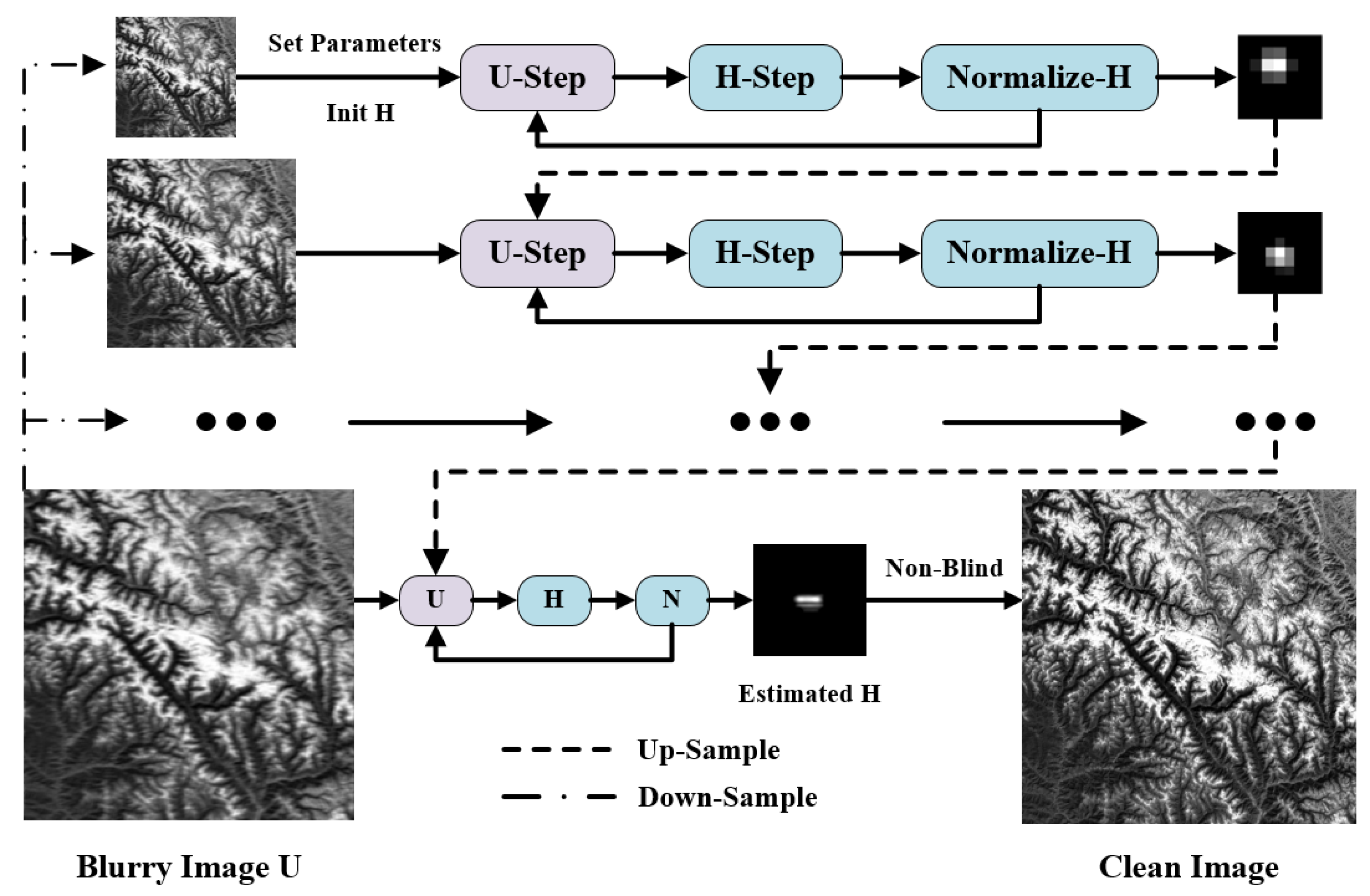
3.4. Estimating the Blur Kernel

Referring to a variety of restoration algorithms [14,15,16,24,25,38], we replace the image intensities in (10) with the image gradients to make the estimated blur kernel more accurate. The formula for solving the blur kernel is:

$$\underset{H}{min}\left|\right|H\otimes \nabla U-{\nabla G\left|\right|}_2^2+{\gamma \left|\right|H\left|\right|}_2^2$$

(27)

The blur kernel can be obtained by using FFT:

$$H=F^{-1}\left(\frac{\overline{F}(\nabla U)F(\nabla G)}{\overline{F}(\nabla U)F(\nabla U)+\gamma }\right)$$

(28)

After obtaining the blur kernel, it needs to be non-negative and normalized:

$$\left\{\begin{array}{c}H(i,j)=0,ifH(i,j)<m·maxH(i,j)\\ {\displaystyle \sum _{\mathsf{\Omega }}}H(i,j)=1\end{array}\right.$$

(29)

where m is the weight. The solution process of the blur kernel is shown in Algorithm 3. Figure 3 is a brief flow-chart of this algorithm.

Algorithm 3: Estimating the blur kernel.

Input: Blurry image G.

Initialize H with results from the coarser level.

While i $\le ma{x}_{i}ter$ do

Solve U using Algorithm 2.

Solve H using Equation (28).

End while

Output: Blur kernel H and intermediate latent image U.

3.5. Algorithm Implementation

This section describes the relevant details that need to be paid attention to in the implementation of this algorithm. In order to get a more accurate blur kernel, we construct a multi-scale image pyramid from coarse-to-fine with a down-sampling factor of $\sqrt{2}/2$, and the total number of cycles of each layer of the pyramid is 5. After estimating the potential clear image U and the blur kernel H, we up-sample the blur kernel H and pass it to the next layer. We usually set $\alpha =0.004-0.012$, $\beta =0.004-0.014$, $\gamma =2$, $ThL=0.5$, $ThM=1$ and $m=0.8$. The number of iterations of the FISTA algorithm is empirically set to 500. These parameters can be adjusted as needed. Finally, a clear image can be obtained after applying the obtained blur kernel to the existing non-blind deblurring method.

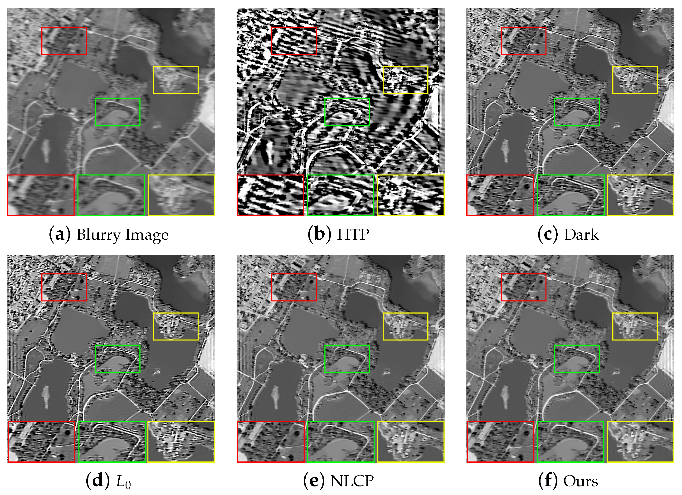
4. Experiment Results

In this paper, the experimental results are divided into simulated and real remote sensing image data. Our method is tested on the AID dataset (http://www.captain-whu.com/project/AID/, accessed on 26 November 2021). The following shows the comparison results of our method with four algorithms, which use the heavy-tailed prior (HTP) [29], the dark channel prior (Dark) [14], $L_0$-regularized intensity and gradient prior ($L_0$) [24] and the non-linear channel prior (NLCP) [16].

4.1. Simulate Remote Sensing Image Data

AID is an aerial image data set composed of sample images collected from Google Earth. The data set consists of the following 30 types of aerial scenes, all of which are marked by experts in the field of remote sensing image interpretation, totaling 10,000 images. In the test experiment of simulated remote sensing images, we selected four images from the AID data set to verify the effectiveness of the algorithm, as shown in Figure 4. Taking into account the types of blur in the actual remote sensing images, we added motion blur, Gaussian blur, and defocus blur to the image, respectively, and adopted Peak-Signal-to-Noise Ratio (PSNR), Structural-Similarity (SSIM) [51] and Root Mean Squard Error (RMSE) as judgment indexes.

4.1.1. Motion Blur

We added motion blur with an angle of $0^{\circ }$ and the displacement of 10 pixels to the remote sensing images. The processing results of each method are shown in

Table 1. Quantitative Comparisons on Remote Sensing Image with Motion Blur.

Method	Figure 4a			Figure 4b
	PSNR	SSIM	RMSE	PSNR	SSIM	RMSE
HTP [29]	22.9257	0.7882	$1.71\times {10}^{-4}$	15.5394	0.51	$1.28\times {10}^{-4}$
Dark [14]	24.9247	0.8343	$2.08\times {10}^{-4}$	8.7337	0.1263	$\mathbf{5}.\mathbf{94}\times {\mathbf{10}}^{-\mathbf{5}}$
${\mathit{L}}_{\mathbf{0}}$ [24]	17.389	0.6035	$2.81\times {10}^{-4}$	9.6171	0.2032	$7.51\times {10}^{-5}$
NLCP [16]	26.0395	0.8514	$1.55\times {10}^{-4}$	10.8196	0.3499	$2.67\times {10}^{-4}$
Ours	26.4378	0.8547	$\mathbf{6}.\mathbf{02}\times {\mathbf{10}}^{-\mathbf{5}}$	16.096	0.5591	$1.71\times {10}^{-4}$
Method	Figure 4c			Figure 4d
	PSNR	SSIM	RMSE	PSNR	SSIM	RMSE
HTP [29]	29.8503	0.8088	$\mathbf{7}.\mathbf{07}\times {\mathbf{10}}^{-\mathbf{5}}$	4.3138	0.0565	$8.78\times {10}^{-4}$
Dark [14]	29.9602	0.8143	$2.14\times {10}^{-4}$	17.9493	0.6659	$2.19\times {10}^{-4}$
${\mathit{L}}_{\mathbf{0}}$ [24]	25.1494	0.7386	$2.43\times {10}^{-4}$	14.139	0.534	$2.52\times {10}^{-4}$
NLCP [16]	28.9047	0.7755	$2.45\times {10}^{-4}$	23.4888	0.8028	$1.91\times {10}^{-4}$
Ours	30.1424	0.8163	$2.04\times {10}^{-4}$	25.6768	0.8427	$\mathbf{2}.\mathbf{07}\times {\mathbf{10}}^{-\mathbf{6}}$

. HTP can sharpen the main contour edges of the image very well, but its ability to retain the details of the image is poor. Furthermore, the images processed by HTP have artifacts remaining. Dark and $L_0$ use $L_0$-norm processing for the prior items of images, which leads to the problem of the over-sharpening of the image. This phenomenon is grave when facing remote sensing images with complex texture details. NLCP and our method use convex $L_1$-norm accumulation for the prior terms of the image. The processing results have good visual effects and will not appear to have over-sharpening like Dark and $L_0$, but the PSNR, SSIM and RMSE of our method are better. However, for Figure 4b with too many details, NLCP sharpens the tiny details in the image and makes the resulting image quality degraded. In general, our method performs well in processing remote sensing images with motion blur. Figure 5 and Figure 6 show representative images of the processing results.

4.1.2. Gaussian Blur

For Gaussian blur, we set its size to 20 × 20 and standard deviation to 0.5. The evaluation results of each method are shown in

Table 2. Quantitative Comparisons on Remote Sensing Image with Gaussian Blur.

Method	Figure 4a			Figure 4b
	PSNR	SSIM	RMSE	PSNR	SSIM	RMSE
HTP [29]	16.0017	0.5744	$9.71\times {10}^{-4}$	15.0446	0.5493	$2.38\times {10}^{-4}$
Dark [14]	12.0795	0.4805	$3.46\times {10}^{-4}$	1.2252	0.0336	$4.41\times {10}^{-4}$
${\mathit{L}}_{\mathbf{0}}$ [24]	10.3751	0.4253	$4.18\times {10}^{-4}$	1.1397	0.0072	$4.24\times {10}^{-4}$
NLCP [16]	21.32	0.8159	$3.88\times {10}^{-4}$	11.8677	0.4549	$4.76\times {10}^{-4}$
Ours	22.4017	0.8094	$\mathbf{1}.\mathbf{71}\times {\mathbf{10}}^{-\mathbf{4}}$	16.8765	0.6564	$\mathbf{8}.\mathbf{93}\times {\mathbf{10}}^{-\mathbf{5}}$
Method	Figure 4c			Figure 4d
	PSNR	SSIM	RMSE	PSNR	SSIM	RMSE
HTP [29]	27.0649	0.7649	$\mathbf{7}.\mathbf{71}\times {\mathbf{10}}^{-\mathbf{5}}$	-4.3236	0.0012	$5.86\times {10}^{-4}$
Dark [14]	24.927	0.6602	$1.55\times {10}^{-4}$	11.4001	0.4046	$1.18\times {10}^{-4}$
${\mathit{L}}_{\mathbf{0}}$ [24]	14.5766	0.2655	$2.11\times {10}^{-4}$	7.5502	0.3127	$4.96\times {10}^{-5}$
NLCP [16]	27.4396	0.7738	$1.45\times {10}^{-4}$	20.1692	0.7744	$3.40\times {10}^{-5}$
Ours	31.1574	0.9026	$1.37\times {10}^{-5}$	23.2932	0.8725	$\mathbf{2}.\mathbf{62}\times {\mathbf{10}}^{-\mathbf{5}}$

. Through observation, it can be seen that the performance of each method in processing Gaussian blur is similar to that in processing motion blur. The images processed by HTP lack detailed information. Dark and $L_0$ are more serious damage to images with rich details. NLCP performs well in most cases and achieves results consistent with the subjective vision of our method. However, when processing Figure 4b with too many details, it still sharpens the tiny details in the image, which greatly reduces the evaluation of visual effects and objective indicators. In general, in the process of removing the Gaussian blur of the remote sensing image, the restored images of our method achieve good visual effects and objective indicators. Figure 7 and Figure 8 show representative images of the processing results.

4.1.3. Defocus Blur

We added defocus blur with a radius of 2 to the remote sensing image. The evaluation results of each method are shown in

Table 3. Quantitative Comparisons on Remote Sensing Image with Defocus Blur.

Method	Figure 4a			Figure 4b
	PSNR	SSIM	RMSE	PSNR	SSIM	RMSE
HTP [29]	24.5929	0.8585	$7.68\times {10}^{-5}$	21.2477	0.7874	$1.10\times {10}^{-4}$
Dark [14]	25.7106	0.868	$9.54\times {10}^{-5}$	6.528	0.0915	$1.55\times {10}^{-4}$
${\mathit{L}}_{\mathbf{0}}$ [24]	20.6962	0.759	$6.79\times {10}^{-5}$	10.413	0.3589	$2.42\times {10}^{-4}$
NLCP [16]	27.2596	0.892	$2.45\times {10}^{-5}$	21.3035	0.7968	$1.29\times {10}^{-4}$
Ours	27.6087	0.8957	$\mathbf{2}.\mathbf{40}\times {\mathbf{10}}^{-\mathbf{5}}$	21.7349	0.8063	$\mathbf{1}.\mathbf{09}\times {\mathbf{10}}^{-\mathbf{4}}$
Method	Figure 4c			Figure 4d
	PSNR	SSIM	RMSE	PSNR	SSIM	RMSE
HTP [29]	30.548	0.843	$\mathbf{9}.\mathbf{77}\times {\mathbf{10}}^{-\mathbf{5}}$	1.7656	0.0195	$2.50\times {10}^{-3}$
Dark [14]	31.7588	0.8616	$1.60\times {10}^{-4}$	21.7453	0.781	$8.82\times {10}^{-5}$
${\mathit{L}}_{\mathbf{0}}$ [24]	30.6986	0.8476	$1.82\times {10}^{-4}$	16.2103	0.6318	$6.96\times {10}^{-5}$
NLCP [16]	30.2685	0.8337	$1.39\times {10}^{-4}$	27.5728	0.8918	$9.69\times {10}^{-5}$
Ours	32.1723	0.8699	$1.73\times {10}^{-4}$	27.8422	0.8991	$\mathbf{8}.\mathbf{08}\times {\mathbf{10}}^{-\mathbf{5}}$

. Through observation, it can be seen that HTP cannot retain the detailed information of the image. Except for Figure 4b, the results of Dark processing have no obvious over-sharpening phenomenon. The result has excellent evaluation indexes, especially when Dark deals with Figure 4c with scarce detail information. The performance of NLCP is very stable and can achieve good results in most cases. Overall, for processing remote sensing images with defocus blur, the images processed by our method and NLCP achieve excellent visual effects compared to other methods, but our method achieves higher objective metrics. Figure 9 and Figure 10 show a representative image of the processing result.

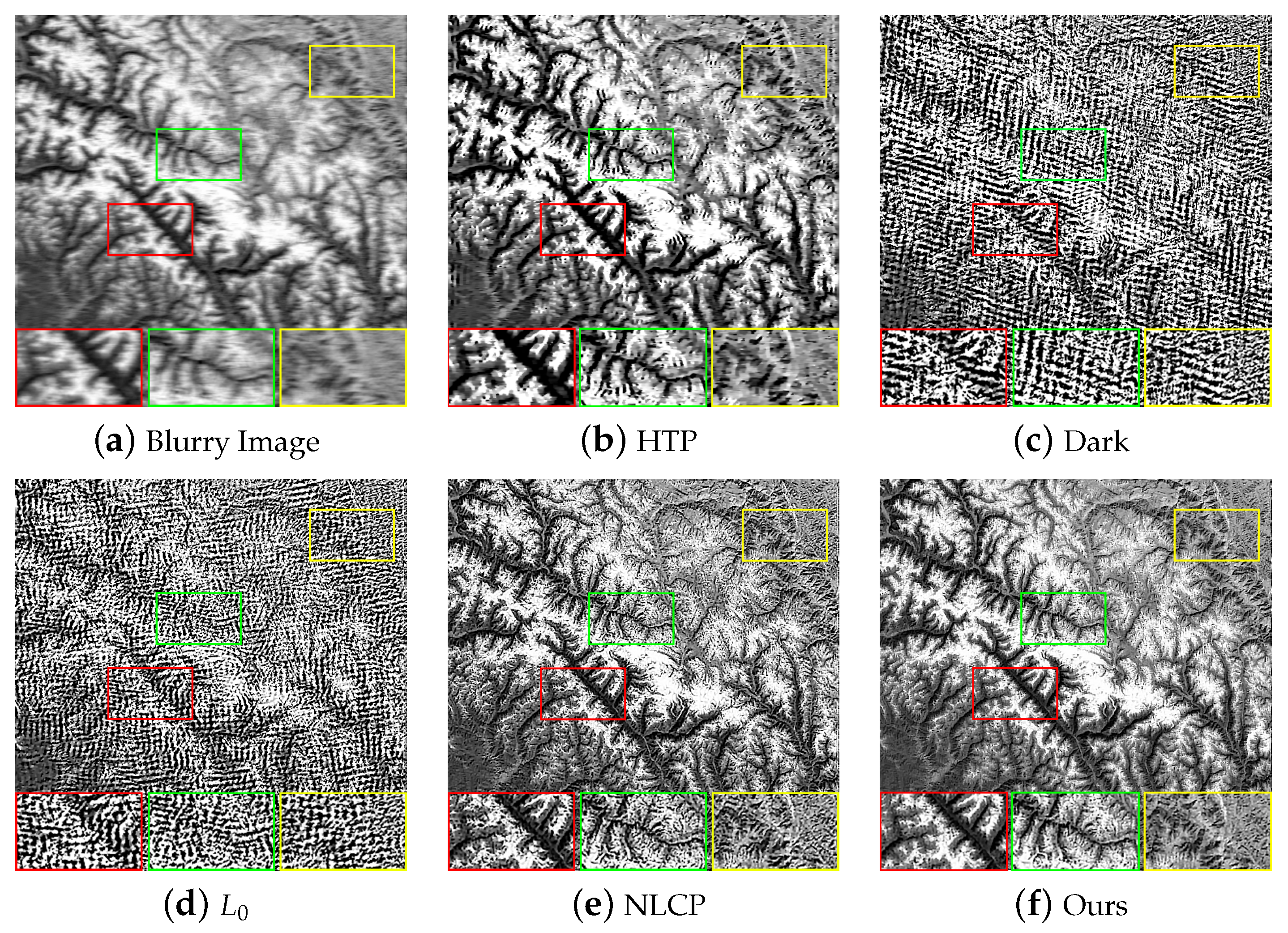
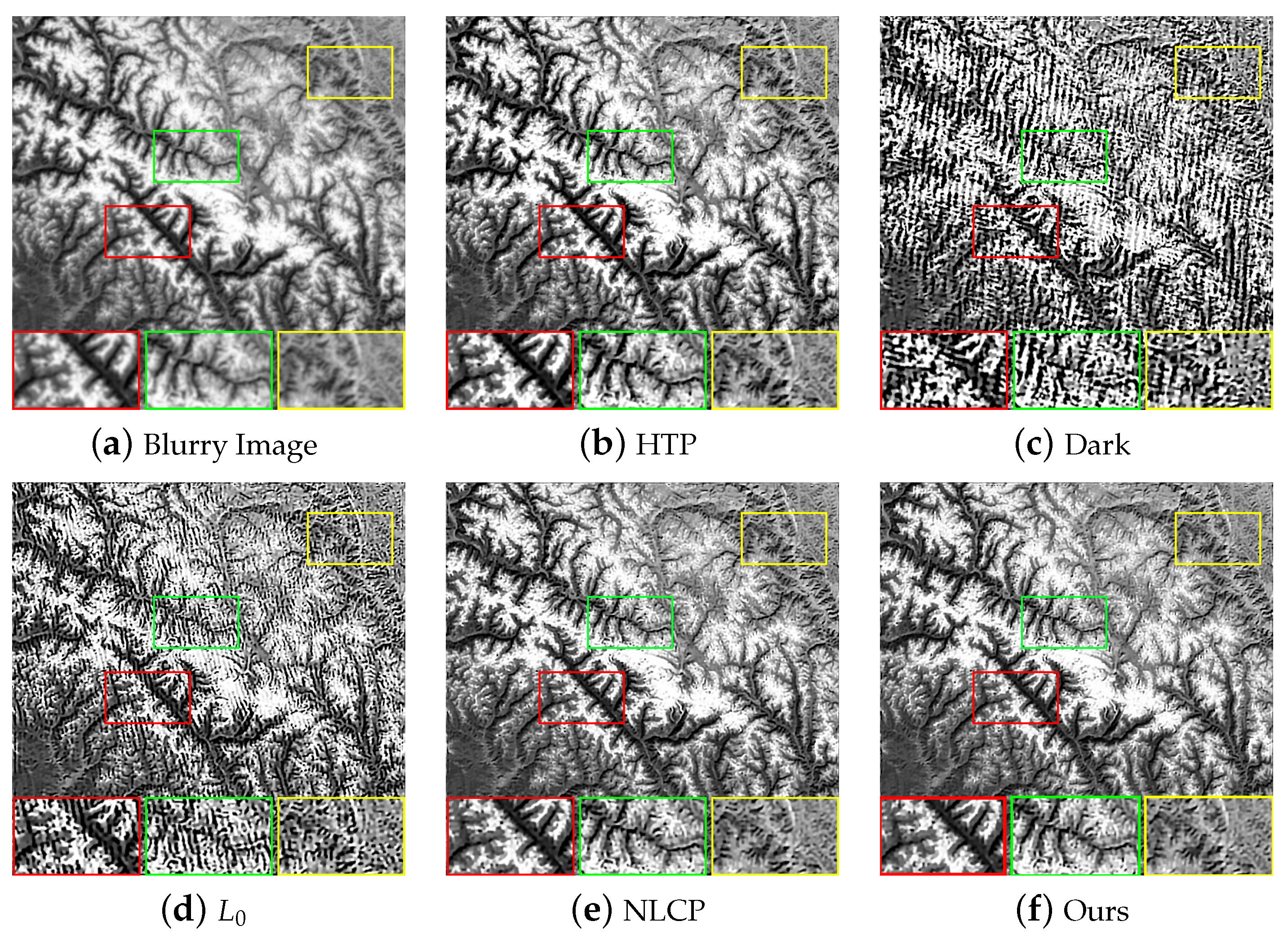
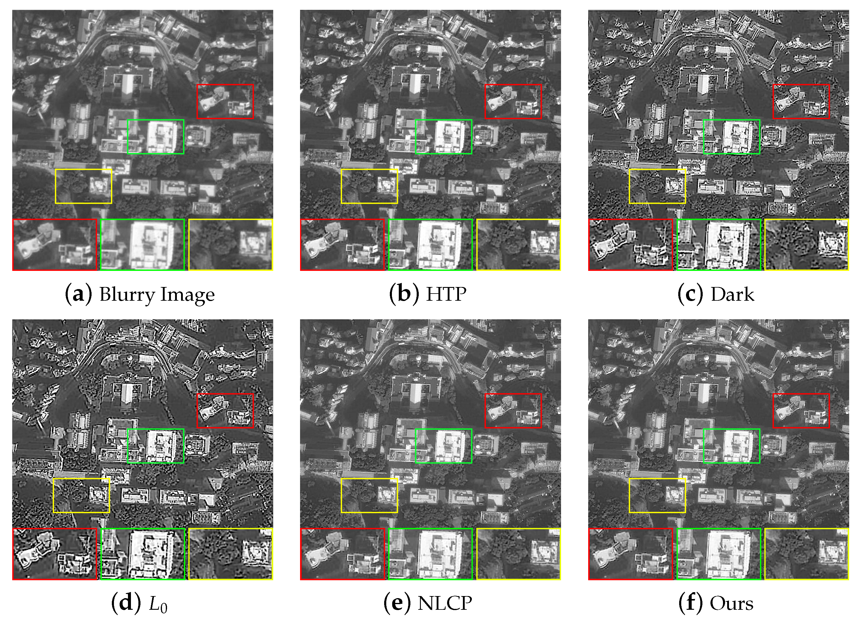
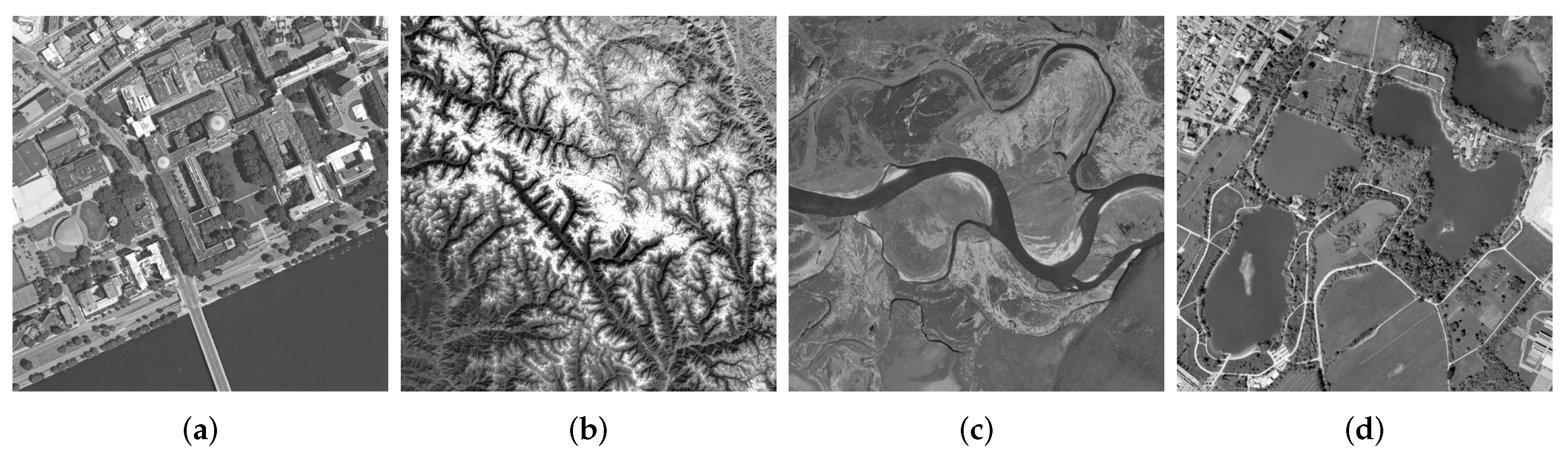
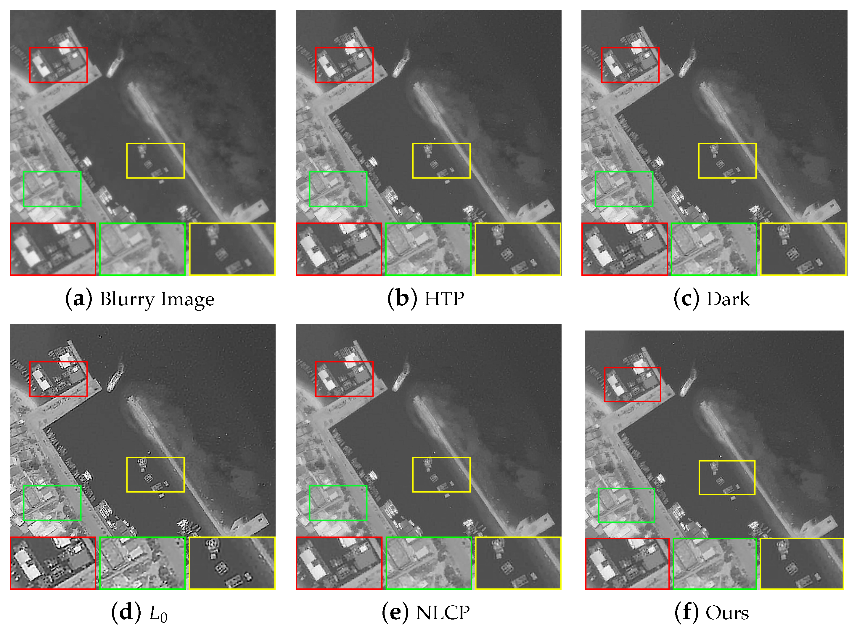
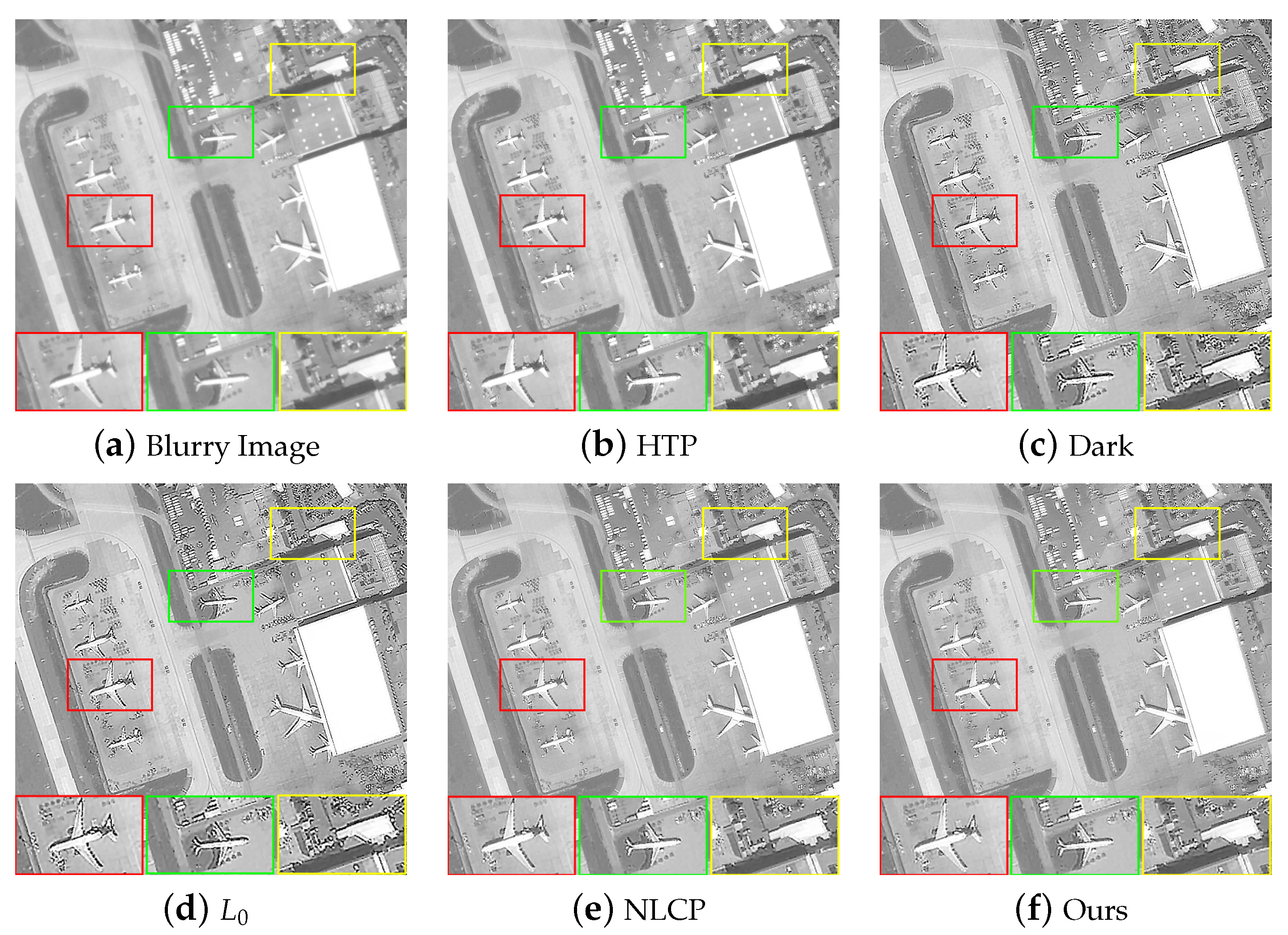
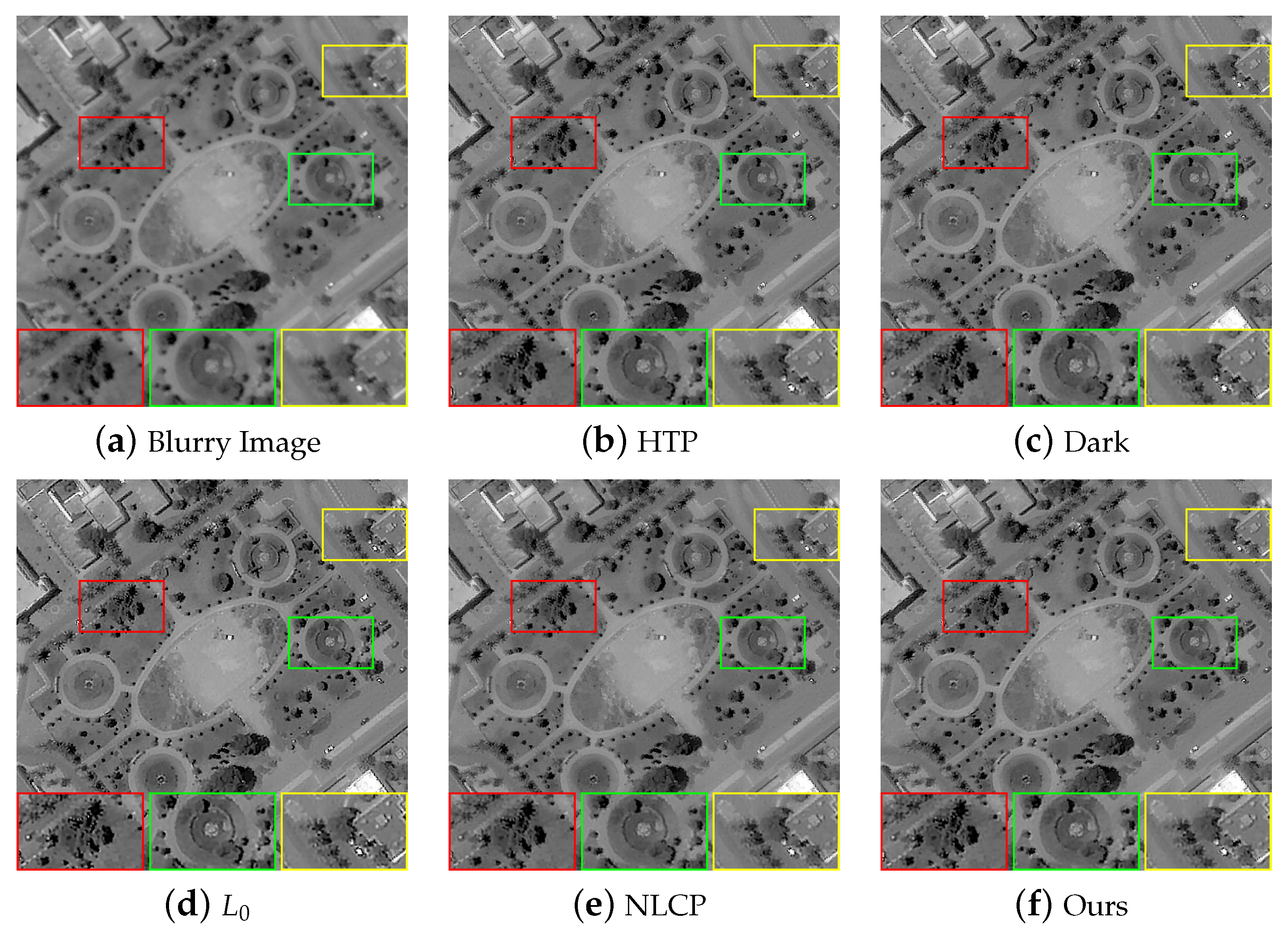
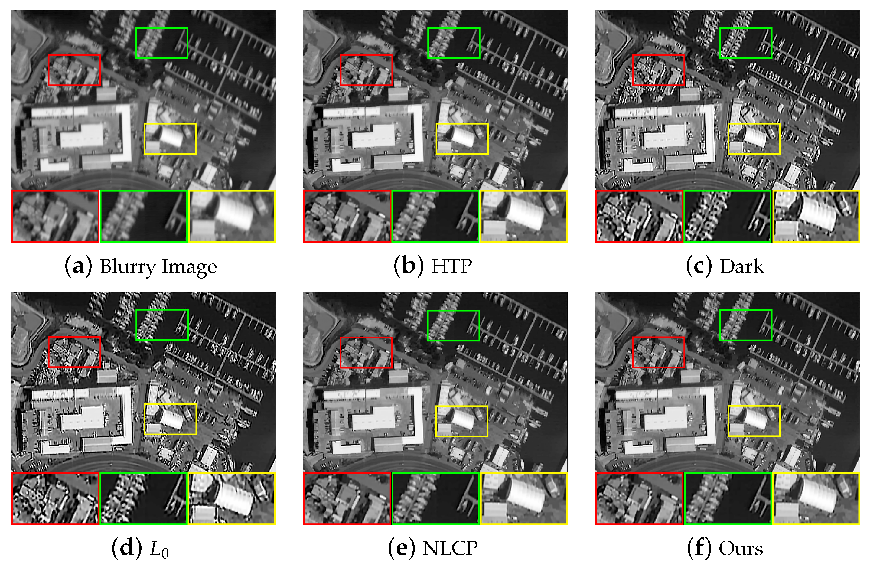
4.2. Real Remote Sensing Image Data

In the real remote sensing images test experiment, we selected four blurry images from the AID data set (Figure 11a–d) and a target image was taken in the experiment (Figure 11e), as shown in Figure 11, to test the effectiveness of our algorithm. In this case, there are no reference images, so we need to apply the no-reference image sharpness assessment indexes. The evaluation indexes include image Entropy (E) [52], Average Gradient (AG) and Point sharpness (P) [53]. Through the comparison of

Table 4. Quantitative Comparisons on Real Remote Sensing Image.

Method	Figure 11a			Figure 11b			Figure 11c			Figure 11d
	E	AG	P	E	AG	P	E	AG	P	E	AG	P
HTP [29]	6.4787	0.0153	0.1057	6.8137	0.041	0.285	7.1373	0.0357	0.2412	6.9637	0.0224	0.1553
Dark [14]	6.4757	0.0181	0.1263	6.9836	0.0968	0.6781	7.2132	0.0925	0.6286	6.9755	0.0267	0.1833
${\mathit{L}}_{\mathbf{0}}$ [24]	6.5899	0.0316	0.2196	6.9261	0.1269	0.8879	7.2365	0.1072	0.7283	6.9977	0.0328	0.2266
NLCP [16]	6.4623	0.0168	0.1156	6.8072	0.0459	0.3182	7.2153	0.0587	0.3963	6.9682	0.0249	0.1715
Ours	6.4846	0.0174	0.1198	6.8149	0.0472	0.3274	7.2242	0.0589	0.3989	6.9865	0.0267	0.1848

and

Table 5. Quantitative Comparisons on Experimental Target Image.

Method	E	AG	P
HTP [29]	7.2031	0.0352	0.2448
Dark [14]	7.1581	0.0976	0.6845
${\mathit{L}}_{\mathbf{0}}$ [24]	7.1004	0.1023	0.7172
NLCP [16]	7.2145	0.0408	0.2828
Ours	7.2286	0.0441	0.3066

, Figure 12, Figure 13, Figure 14, Figure 15 and Figure 16, it is clear that HTP restores the overall outline of the image very well but lacks the ability to retain detailed information. The processing results of Dark and $L0$ algorithms face the problem of over-sharpening. When processing Figure 11a,d with very little texture information, the over-sharpening effect is not obvious, and the resulting image has good visual effects and objective evaluation indicators. However, this effect is particularly serious when dealing with images with many details and scenes (Figure 11b,c,e). The images processed by our algorithm and NLCP can retain more image details, and the visual effects of them are almost the same. However, our algorithm has achieved higher objective evaluation indicators.

5. Analysis and Discussion

In this part, we will test the effectiveness of the LBP prior, the influence of hyper-parameters and the convergence of the algorithm, and discuss our algorithm after sufficient analysis and obtaining experimental results. In all testing experiments, we used the Levin dataset [13] containing four images and eight different blur kernels. All blind image deblurring algorithms, finally, use the same non-blind restoration method to obtain clear images to ensure the reliability of the experiment. In addition, Error-Ratio [13], Peak-Signal-to-Noise Ratio (PSNR), Structural-Similarity (SSIM) [51] and Kernel Similarity [54] are used as quantitative evaluation indicators. All experiments are run on a computer with Intel Core i5-1035G1 CPU and 8 GB RAM.

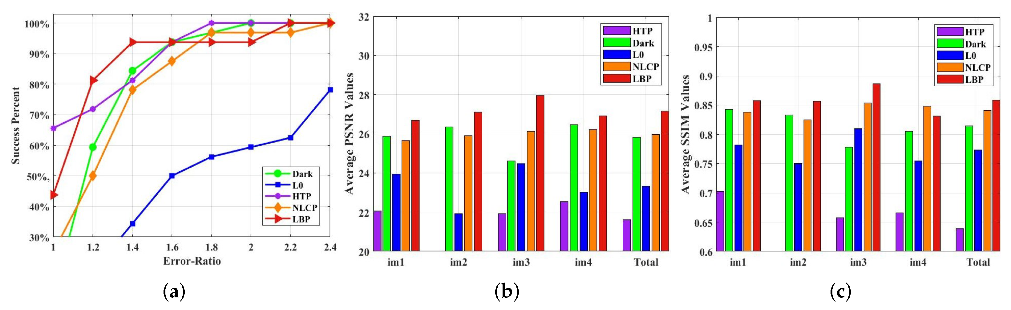
5.1. Effectiveness of the LBP Prior

Although the image deblurring algorithm based on LBP prior can effectively obtain a clear image in theory, it needs to be quantitatively evaluated and verified in the actual situation. As shown in Figure 17, the proposed algorithm is compared with HTP [29], Dark [14], $L_0$ [24] and NLCP [16]. The performance of our algorithm in error accumulation rate is second only to MAP, and it is better than other methods in the two indicators of average PSNR and average SSIM. Overall, LBP prior can effectively remove the blur in the image and improve the image quality.

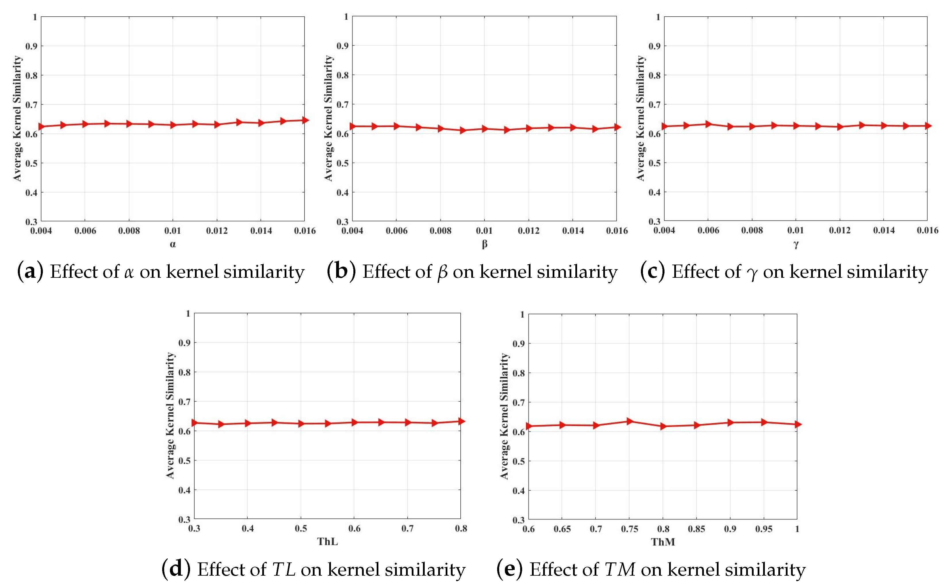
5.2. Effect of Hyper-Parameters

The objective function (8) proposed in this paper mainly contains five main hyper-parameters, i.e., $\alpha$, $\beta$, $\gamma$, $ThL$, and $ThM$. To explore the influence of the five hyper-parameters on the proposed algorithm, we only changed one parameter at a time, ensuring that other parameters remained unchanged, and then calculated the kernel similarity between the estimated blur kernel and the ground truth kernel. Suppose the kernel similarity does not change on a large scale with the change of hyper-parameters. In that case, the estimated blur kernel is relatively stable, i.e., the algorithm is not sensitive to hyper-parameters. As shown in Figure 18, our method is not sensitive to changes in a wide range of hyper-parameters.

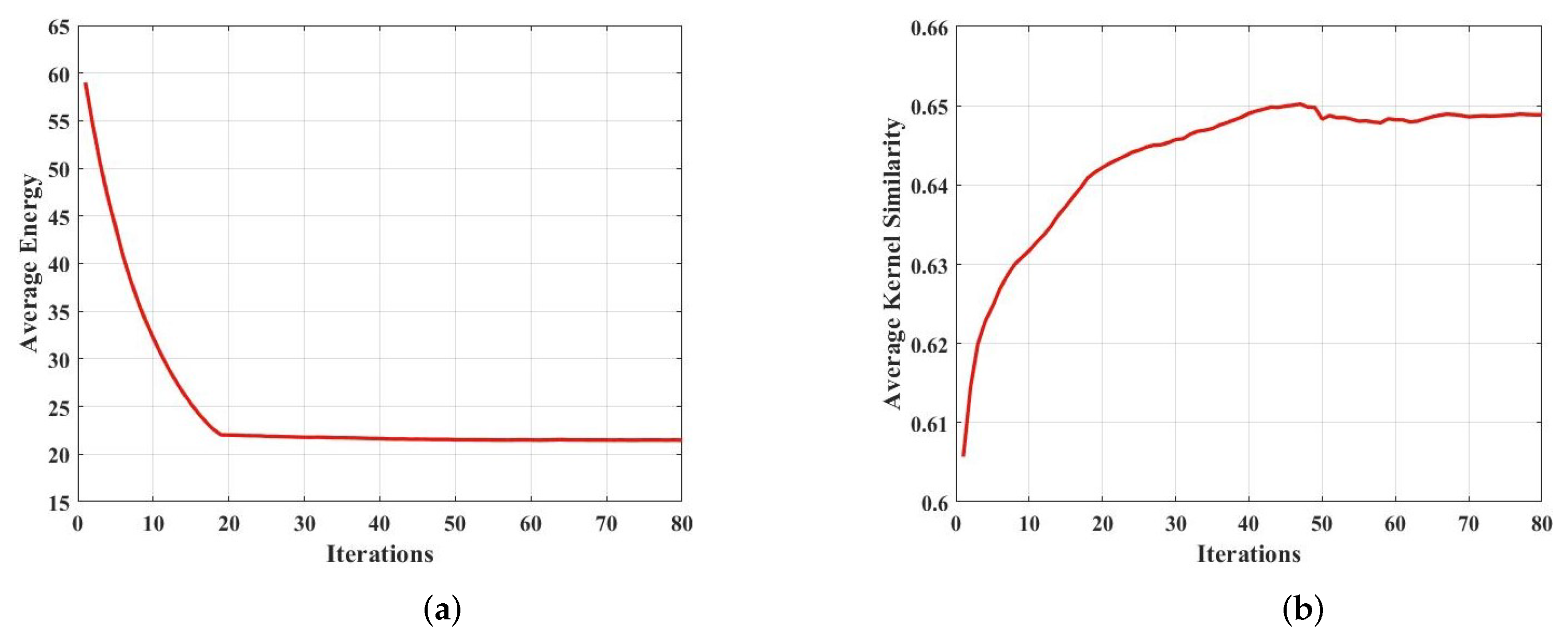
5.3. Convergence Analysis

PAM is widely used in various algorithms as an effective method to make the objective function converge to the optimal solution. For the convergence of the PAM method applied to the total variational algorithm, reference [6] gives an explanation of delay scaling (normalization) in the iterative step of the blur kernel. Our algorithm also applies the PAM method and uses half-quadratic splitting method to decompose the objective function into several sub-problems. It is known that each sub-problem has a convergent solution [18,55], but the overall theoretical research on convergence is minimal. The convergence of the algorithm can be quantitatively verified by calculating the average energy function (8) and the average kernel similarity that changes with iteration under the optimal scale of the Levin dataset. As shown in Figure 19, our method converges after approximately 19 iterations, and the kernel similarity stabilizes after 40 iterations, proving the method’s convergence.

5.4. Run-Time Comparisons

To explore the running efficiency of each algorithm, we tested the average running time of different restoration algorithms. The test results are shown in

Table 6. Running Time (in second) Comparison.

Method	125 × 125	255 × 255	600 × 600
HTP [29]	78.44	85.62	114.55
Dark [14]	72.84	220.91	870.64
${\mathit{L}}_{\mathbf{0}}$ [24]	13.53	40.81	198.82
NLCP [16]	32.44	131.98	570.39
Ours	20.2	70.51	364.37

. By comprehensively analyzing the data in Table 6 and the conclusions in Section 5.1, it is clear that our method achieves very competitive processing results while spending relatively less time.

5.5. Limitations

Although our method excels in processing remote sensing images, it has limitations. The hyper-parameters used by our algorithm are not fixed due to the introduction of LBP priors. To achieve the best processing effect, it is necessary to select corresponding parameters for different processed images. In addition, the presence of noise in the image will also affect the processing effect. Significant noise, especially the strip noise that often appears in remote sensing imaging, will make our method misjudge important pixels and amplify the noise. At the same time, to get a clear image, our algorithm uses PAM, which includes the half-quadratic splitting method and FISTA, to solve the objective function, and updates the parameters iteratively. This way of solving will undoubtedly increase the amount of calculation and make the whole process more time-consuming. Therefore, for future work, we will focus on exploring the factors affecting the hyper-parameters to improve the LBP prior further, using the LBP prior to remove noise and blur at the same time and reducing the amount of calculation to shorten the processing time.

6. Conclusions

Unlike the existing methods dedicated to exploring the prior that can clearly distinguish between a clear image and the blurry image, the prior we introduce is used to select critical pixels to restore images by focusing on the similarities. The proposed algorithm uses LBP, to filter pixels because of remote sensing images with small scenes and numerous details. It processes different types of pixels, respectively, to prevent over-sharpening while restoring the images. By introducing the LBP prior, we established an optimization model based on PAM, which involves the construction of the mapping matrix, the fast iterative shrinkage-thresholding algorithm (FISTA) and the half-quadratic splitting method. It can be seen that the proposed algorithm has excellent convergence and stability. The experimental results show that our method is better than the existing algorithms for deblurring remote sensing images. Moreover, we believe that the proposed algorithm can provide a new idea for further developing remote sensing image processing.

References

1. Rugna, J.D.; Konik, H. Automatic blur detection for metadata extraction in content-based retrival context. In Proceedings of the Internet Imaging V SPIE, San Jose, CA, USA, 18–22 January 2004; Volume 5304, pp. 285–294. [Google Scholar]
2. Liu, R.T.; Li, Z.R.; Jia, J.Y. Image partial blur detection and classification. In Proceedings of the 2008 IEEE Conference on Computer Vision and Pattern Recognition, Anchorage, AK, USA, 23–28 June 2008; pp. 1–8. [Google Scholar]
3. Rudin, L.I.; Osher, S.; Fatemi, E. Nonlinear total variation based noise removal algorithms. Phys. D Nonlinear Phenom. 1992, 60, 259–268. [Google Scholar] [CrossRef]
4. Chan, T.F.; Wong, C.-K. Total variation blind deconvolution. IEEE Trans. Image Process. 1998, 7, 370–375. [Google Scholar] [CrossRef] [PubMed] [Green Version]
5. Liao, H.Y.; Ng, M.K. Blind deconvolution using generalized cross-validation approach to regularization parameter estimation. IEEE Trans. Image Process. 2011, 20, 670–680. [Google Scholar] [CrossRef] [PubMed]
6. Perrone, D.; Favaro, P. Total variation blind deconvolution: The Devil Is in the Details. In Proceedings of the 2014 IEEE Conference on Computer Vision and Pattern Recognition, Columbus, OH, USA, 23–28 June 2014; pp. 2909–2916. [Google Scholar]
7. Rameshan, R.M.; Chaudhuri, S.; Velmurugan, R. Joint MAP estimation for blind deconvolution: When does it work? In Proceedings of the Eighth Indian Conference on Computer Vision, Graphics and Image Processing December, Mumbai, India, 16–19 December 2012; pp. 1–7. [Google Scholar]
8. Likas, A.C.; Galatsanos, N.P. A variational approach for Bayesian blind image deconvolution. IEEE Trans. Signal Process. 2004, 52, 2222–2233. [Google Scholar] [CrossRef]
9. Fergus, R.; Singh, B.; Hertzmann, A.; Roweis, S.T.; Freeman, W.T. Removing camera shake from a single photograph. In Proceedings of the SIGGRAPH06: Special Interest Group on Computer Graphics and Interactive Techniques Conference, Boston, MA, USA, 30 July–3 August 2006; pp. 787–794. [Google Scholar]
10. Levin, A.; Weiss, Y.; Durand, F.; Freeman, W.T. Efficient marginal likelihood optimization in blind deconvolution. In Proceedings of the CVPR 2011, Colorado Springs, CO, USA, 20–25 June 2011; pp. 2657–2664. [Google Scholar]
11. Wipf, D.; Zhang, H.C. Analysis of Bayesian blind deconvolution. In Proceedings of the Energy Minimization Methods in Computer Vision and Pattern Recognition, Lund, Sweden, 19–21 August 2013; pp. 40–53. [Google Scholar]
12. Perrone, D.; Diethelm, R.; Favaro, P. Blind deconvolution via lower bounded logarithmic image priors. In Proceedings of the 10th International Conference EMMCVPR 2015, Hong Kong, China, 13–16 January 2015; pp. 112–125. [Google Scholar]
13. Levin, A.; Weiss, Y.; Durand, F.; Freeman, W.T. Understanding and evaluating blind deconvolution algorithms. In Proceedings of the 2009 IEEE Conference on Computer Vision and Pattern Recognition, Miami, FL, USA, 20–25 June 2009; pp. 1964–1971. [Google Scholar]
14. Pan, J.S.; Sun, D.Q.; Pfister, H.; Yang, M.-H. Blind image deblurring using dark channel prior. In Proceedings of the 2016 IEEE Conference on Computer Vision and Pattern Recognition (CVPR), Las Vegas, NV, USA, 27–30 June 2016; pp. 1628–1636. [Google Scholar]
15. Yan, Y.Y.; Ren, W.Q.; Guo, Y.F.; Wang, R.; Cao, X.C. Image deblurring via extreme channels prior. In Proceedings of the 2017 IEEE Conference on Computer Vision and Pattern Recognition (CVPR), Honolulu, HI, USA, 21–26 July 2017; pp. 6978–6986. [Google Scholar]
16. Ge, X.Y.; Tan, J.Q.; Zhang, L. Blind Image Deblurring Using a Non-Linear Channel Prior Based on Dark and Bright Channels. IEEE Trans. Image Process. 2021, 30, 6970–6984. [Google Scholar] [CrossRef]
17. Ojala, T.; Pietikäinen, M.; Harwood, D. A comparative study of texture measures with classification based on featured distributions. Pattern Recognit. 1996, 29, 51–59. [Google Scholar] [CrossRef]
18. Beck, A.; Teboulle, M. A fast iterative shrinkage-thresholding algorithm for linear inverse problems. SIAM J. Imaging Sci. 2009, 2, 183–202. [Google Scholar] [CrossRef] [Green Version]
19. Joshi, N.; Szeliski, R.; Kriegman, D.J. PSF estimation using sharp edge prediction. In Proceedings of the 2008 IEEE Conference on Computer Vision and Pattern Recognition (CVPR), Anchorage, AK, USA, 23–28 June 2008; pp. 1–8. [Google Scholar]
20. Cho, S.; Lee, S. Fast motion deblurring. ACM Trans. Graph. 2009, 28, 1–8. [Google Scholar] [CrossRef]
21. Xu, L.; Jia, J.Y. Two-phase kernel estimation for robust motion deblurring. In Proceedings of the 11th European Conference on Computer Vision: Part I, Heraklion, Crete, Greece, 5–11 September 2010; pp. 157–170. [Google Scholar]
22. Sun, L.B.; Cho, S.; Wang, J.; Hays, J. Edge-based blur kernel estimation using patch priors. In Proceedings of the IEEE International Conference on Computational Photography (ICCP), Cambridge, MA, USA, 19–21 April 2013; pp. 1–8. [Google Scholar]
23. Ren, W.Q.; Cao, X.C.; Pan, J.S.; Guo, X.J.; Zuo, W.M.; Yang, M.-H. Image deblurring via enhanced low-rank prior. IEEE Trans. Image Process. 2016, 25, 3426–3437. [Google Scholar] [CrossRef]
24. Pan, J.S.; Hu, Z.; Su, Z.X.; Yang, M.-H. L0-Regularized Intensity and Gradient Prior for Deblurring Text Images and Beyond. IEEE Trans. Pattern Anal. Mach. Intell. 2017, 39, 342–355. [Google Scholar] [CrossRef]
25. Chen, L.; Fang, F.M.; Wang, T.T.; Zhang, G.X. Blind image deblurring with local maximum gradient prior. In Proceedings of the 2019 IEEE/CVF Conference on Computer Vision and Pattern Recognition (CVPR), Long Beach, CA, USA, 15–20 June 2019; pp. 1742–1750. [Google Scholar]
26. Yuzuriha, R.; Kurihara, R.; Matsuoka, R.; Okuda, M. TNNG: Total Nuclear Norms of Gradients for Hyperspectral Image Prior. Remote Sens. 2021, 13, 819. [Google Scholar] [CrossRef]
27. Shan, Q.; Jia, J.; Agarwala, A. High-quality motion deblurring from a single image. ACM Trans. Graph. 2008, 27, 1–10. [Google Scholar]
28. Krishnan, D.; Tay, T.; Fergus, R. Blind deconvolution using a normalized sparsity measure. In Proceedings of the CVPR 2011, Colorado Springs, CO, USA, 20–25 June 2011; pp. 233–240. [Google Scholar]
29. Kotera, J.; Šroubek, F.; Milanfar, P. Blind Deconvolution Using Alternating Maximum a Posteriori Estimation with Heavy-Tailed Priors. In Proceedings of the 15th International Conference on Computer Analysis of Images and Patterns (CAIP), York, UK, 27–29 August 2013; pp. 59–66. [Google Scholar]
30. Michaeli, T.; Irani, M. Blind deblurring using internal patch recurrence. In Proceedings of the 13th European Conference on Computer Vision, Zurich, Switzerland, 6–12 September 2014; pp. 783–798. [Google Scholar]
31. Zhong, Q.X.; Wu, C.S.; Shu, Q.L.; Liu, W. Spatially adaptive total generalized variation-regularized image deblurring with impulse noise. J. Electron. Imaging 2018, 27, 1–21. [Google Scholar] [CrossRef]
32. Yang, D.Y.; Wu, X.J. Dual-Channel Contrast Prior for Blind Image Deblurring. IEEE Access 2020, 8, 227879–227893. [Google Scholar] [CrossRef]
33. Liu, J.; Tan, J.Q.; He, L.; Ge, X.Y.; Hu, D.D. Blind Image Deblurring via Local Maximum Difference Prior. IEEE Access 2020, 8, 219295–219307. [Google Scholar] [CrossRef]
34. Zhou, L.Y.; Liu, Z.Y. Blind Deblurring Based on a Single Luminance Channel and L1-Norm. IEEE Access 2021, 9, 126717–126727. [Google Scholar] [CrossRef]
35. Chen, L.; Zhang, J.W.; Lin, S.G.; Fang, F.M.; Ren, J.S. Blind Deblurring for Saturated Images. In Proceedings of the 2021 IEEE/CVF Conference on Computer Vision and Pattern Recognition (CVPR), Nashville, TN, USA, 20–25 June 2021; pp. 6304–6312. [Google Scholar]
36. He, W.; Zhang, H.; Zhang, L.; Shen, H. Total-variation-regularized low-rank matrix factorization for hyperspectral image restoration. IEEE Trans. Geosci. Remote Sens. 2016, 54, 178–188. [Google Scholar] [CrossRef]
37. Zhang, H.; He, W.; Zhang, L.; Shen, H.; Yuan, Q. Hyperspectral image restoration using low-rank matrix recovery. IEEE Trans. Geosci. Remote Sens. 2014, 52, 4729–4743. [Google Scholar] [CrossRef]
38. Sun, J.; Cao, W.F.; Xu, Z.B.; Ponce, J. Learning a convolutional neural network for non-uniform motion blur removal. In Proceedings of the 2015 IEEE Conference on Computer Vision and Pattern Recognition (CVPR), Boston, MA, USA, 7–12 June 2015; pp. 769–777. [Google Scholar]
39. Schuler, C.J.; Hirsch, M.; Harmeling, S.; Schölkopf, B. Learning to deblur. IEEE Trans. Pattern Anal. Mach. Intell. 2016, 38, 1439–1451. [Google Scholar] [CrossRef]
40. Li, L.; Pan, J.S.; Lai, W.-S.; Gao, C.X.; Sang, N.; Yang, M.-H. Blind image deblurring via deep discriminative priors. Int. J. Comput. Vis. 2019, 127, 1025–1043. [Google Scholar] [CrossRef]
41. Nah, S.; Kim, T.H.; Lee, K.M. Deep multi-scale convolutional neural network for dynamic scene deblurring. In Proceedings of the 2017 IEEE Conference on Computer Vision and Pattern Recognition (CVPR), Honolulu, HI, USA, 21–26 July 2017; pp. 257–265. [Google Scholar]
42. Cai, J.R.; Zuo, W.M.; Zhang, L. Dark and bright channel prior embedded network for dynamic scene deblurring. IEEE Trans. Image Process. 2020, 29, 6885–6897. [Google Scholar] [CrossRef]
43. Zhang, H.G.; Dai, Y.C.; Li, H.D.; Koniusz, P. Deep stacked hierarchical multi-patch network for image deblurring. In Proceedings of the 2019 IEEE/CVF Conference on Computer Vision and Pattern Recognition (CVPR), Long Beach, CA, USA, 15–20 June 2019; pp. 5971–5979. [Google Scholar]
44. Suin, M.; Purohit, K.; Rajagopalan, A.N. Spatially-attentive patchhierarchical network for adaptive motion deblurring. In Proceedings of the 2020 IEEE/CVF Conference on Computer Vision and Pattern Recognition (CVPR), Seattle, WA, USA, 13–19 June 2020; pp. 3603–3612. [Google Scholar]
45. Lin, T.-Y.; Dollár, P.; Girshick, R.; He, K.M.; Hariharan, B.; Belongie, S. Feature pyramid networks for object detection. In Proceedings of the 2017 IEEE Conference on Computer Vision and Pattern Recognition (CVPR), Honolulu, HI, USA, 21–26 July 2017; pp. 936–944. [Google Scholar]
46. Li, C.; Gao, W.Z.; Liu, F.H.; Chang, E.B.; Xuan, S.X.; Xu, D.Y. GAMSNet: Deblurring via Generative Adversarial and Multi-Scale Networks. In Proceedings of the 2020 Chinese Automation Congress (CAC), Shanghai, China, 6–8 November 2020; pp. 3631–3636. [Google Scholar]
47. Tian, H.; Sun, L.J.; Dong, X.L.; Lu, B.L.; Qin, H.; Zhang, L.P.; Li, W.J. A Modeling Method for Face Image Deblurring. In Proceedings of the 2021 International Conference on High Performance Big Data and Intelligent Systems (HPBD&IS), Macau, China, 5–7 December 2021; pp. 37–41. [Google Scholar]
48. Maharjan, P.; Xu, N.; Xu, X.; Song, Y.Y.; Li, Z. DCTResNet: Transform Domain Image Deblocking for Motion Blur Images. In Proceedings of the 2021 International Conference on Visual Communications and Image Processing (VCIP), Munich, Germany, 5–8 December 2021; pp. 1–5. [Google Scholar]
49. Chang, M.; Feng, H.J.; Xu, Z.H.; Li, Q. Low-Light Image Restoration with Short- and Long-Exposure Raw Pairs. IEEE Trans. Multimed. 2022, 24, 702–714. [Google Scholar] [CrossRef]
50. Lai, W.S.; Huang, J.B.; Hu, Z.; Ahuja, N.; Yang, M.H. A Comparative Study for Single Image Blind Deblurring. In Proceedings of the 2016 IEEE Conference on Computer Vision and Pattern Recognition (CVPR), Las Vegas, NV, USA, 27–30 June 2016; pp. 1701–1709. [Google Scholar]
51. Wang, Z.; Bovik, A.C.; Sheikh, H.R.; Simoncelli, E.P. Image quality assessment: From error visibility to structural similarity. IEEE Trans. Image Process. 2004, 13, 600–612. [Google Scholar] [CrossRef] [PubMed] [Green Version]
52. Shannon, C.E. A Mathematical Theory of Communication. Bell Syst. Tech. J. 1948, 27, 623–656. [Google Scholar] [CrossRef]
53. Wang, H.N.; Zhong, W.; Wang, J.; Xia, D.S. Research of measurement for digital image definition. J. Image Graph. 2004, 9, 828–831. [Google Scholar]
54. Hu, Z.; Yang, M.-H. Good regions to deblur. In Proceedings of the 12th European Conference on Computer Vision, Florence, Italy, 7–13 October 2012; pp. 59–72. [Google Scholar]
55. Xu, L.; Lu, C.W.; Xu, Y.; Jia, J.Y. Image smoothing via L0 gradient minimization. ACM Trans. Graph. 2011, 30, 1–12. [Google Scholar]
Figure 1. Schematic diagram of LBP feature extraction principle.
Remotesensing 14 01276 g001
Figure 2. Top: A blurry image, corresponding LBP map and LBP normalized distribution histogram. Bottom: The clear image, corresponding LBP map and LBP normalized distribution histogram. (a) Image pair [50]; (b) LBPs; (c) LBP normalized distribution histograms.
Remotesensing 14 01276 g002
Figure 3. A brief flow-chart of this algorithm.
Remotesensing 14 01276 g003
Figure 4. Selected remote sensing image (Simulate).
Remotesensing 14 01276 g004
Figure 5. Visual comparison of remote sensing image (Figure 4a) with motion blur processed by different methods.
Remotesensing 14 01276 g005
Figure 6. Visual comparison of remote sensing image (Figure 4d) with motion blur processed by different methods.
Remotesensing 14 01276 g006
Figure 7. Visual comparison of remote sensing image (Figure 4b) with Gaussian blur processed by different methods.
Remotesensing 14 01276 g007
Figure 8. Visual comparison of remote sensing image (Figure 4c) with Gaussian blur processed by different methods.
Remotesensing 14 01276 g008
Figure 9. Visual comparison of remote sensing image (Figure 4b) with defocus blur processed by different methods.
Remotesensing 14 01276 g009
Figure 10. Visual comparison of remote sensing image (Figure 4d) with defocus blur processed by different methods.
Remotesensing 14 01276 g010
Figure 11. Selected remote sensing image (Real).
Remotesensing 14 01276 g011
Figure 12. Visual comparison of real remote sensing image (Figure 11a) processed by different methods.
Remotesensing 14 01276 g012
Figure 13. Visual comparison of real remote sensing image (Figure 11b) processed by different methods.
Remotesensing 14 01276 g013
Figure 14. Visual comparison of real remote sensing image (Figure 11c) processed by different methods.
Remotesensing 14 01276 g014
Figure 15. Visual comparison of real remote sensing image (Figure 11d) processed by different methods.
Remotesensing 14 01276 g015
Figure 16. Visual comparison of real remote sensing image (Figure 11e) processed by different methods.
Remotesensing 14 01276 g016
Figure 17. Quantitative evaluations on the benchmark dataset [13]. (a) Comparisons in terms of cumulative Error-Ratio. (b) Comparisons in terms of average PSNR. (c) Comparisons in terms of average SSIM.
Remotesensing 14 01276 g017
Figure 18. Sensitivity analysis of hyper-parameters in the proposed method.
Remotesensing 14 01276 g018
Figure 19. Convergence analysis of the proposed method. (a) The average value of the objective function (8). (b) Kernel Similarity.
Remotesensing 14 01276 g019