
Study of the Effect of Vegetation on Reducing Atmospheric Pollution Particles


Abstract
:1. Introduction
2. Materials and Methods
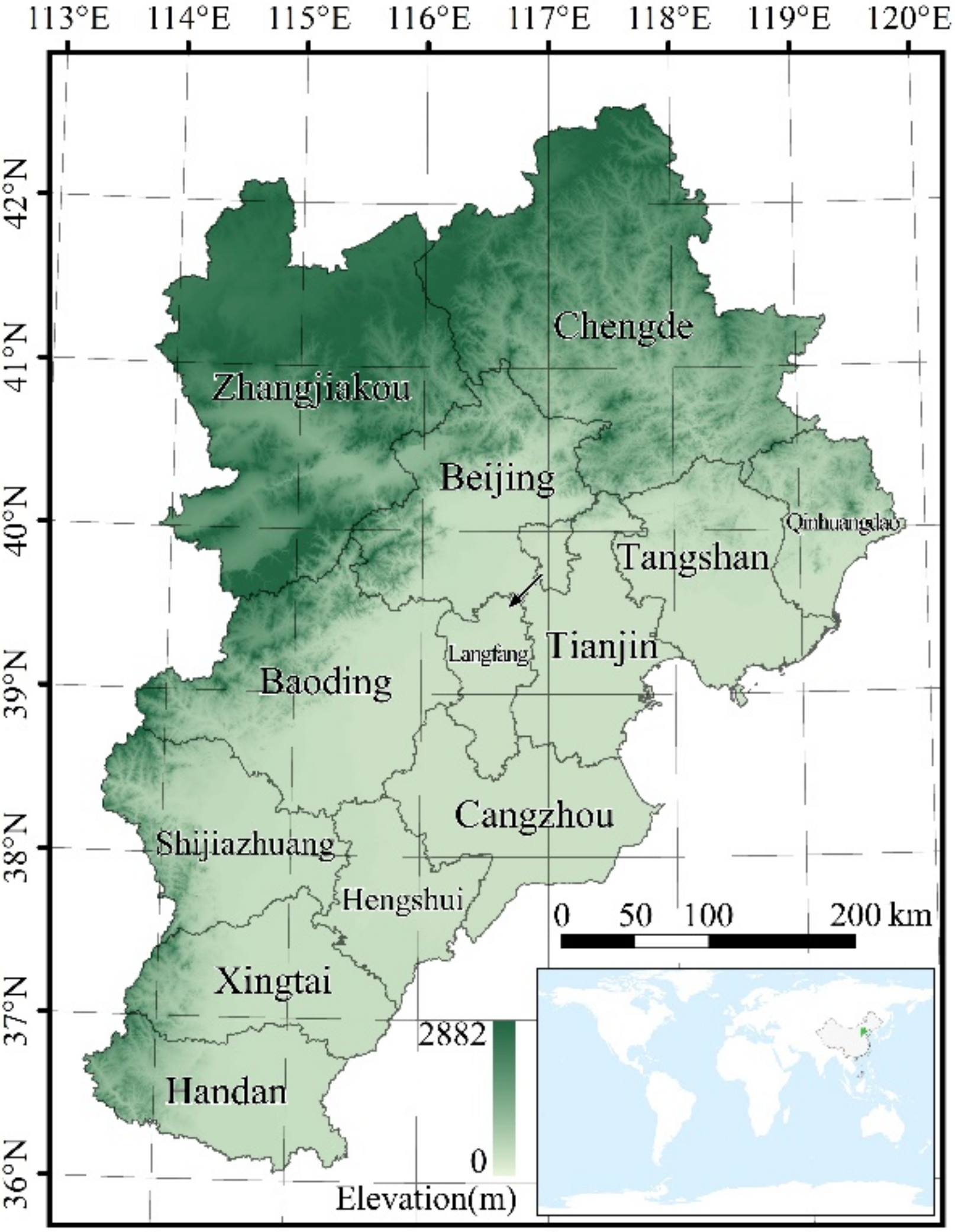
2.1. Overview of the Study Area
2.2. PM Reduction
2.3. Leaf Area Index and Vegetation Coverage Area
2.4. Dry Sedimentation Rate and Resuspension Rate
2.5. Dry Sedimentation Flux
2.6. Assessment of Air Quality Improvement Effect
3. Experiment
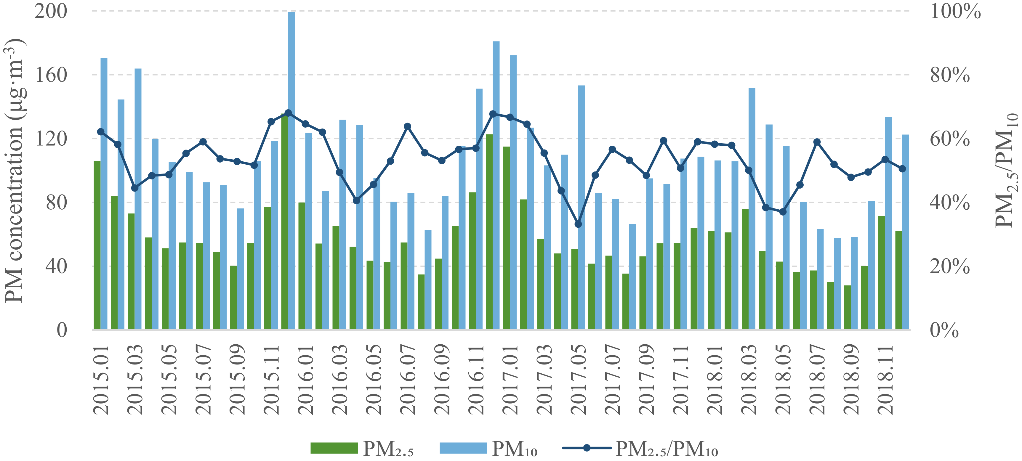
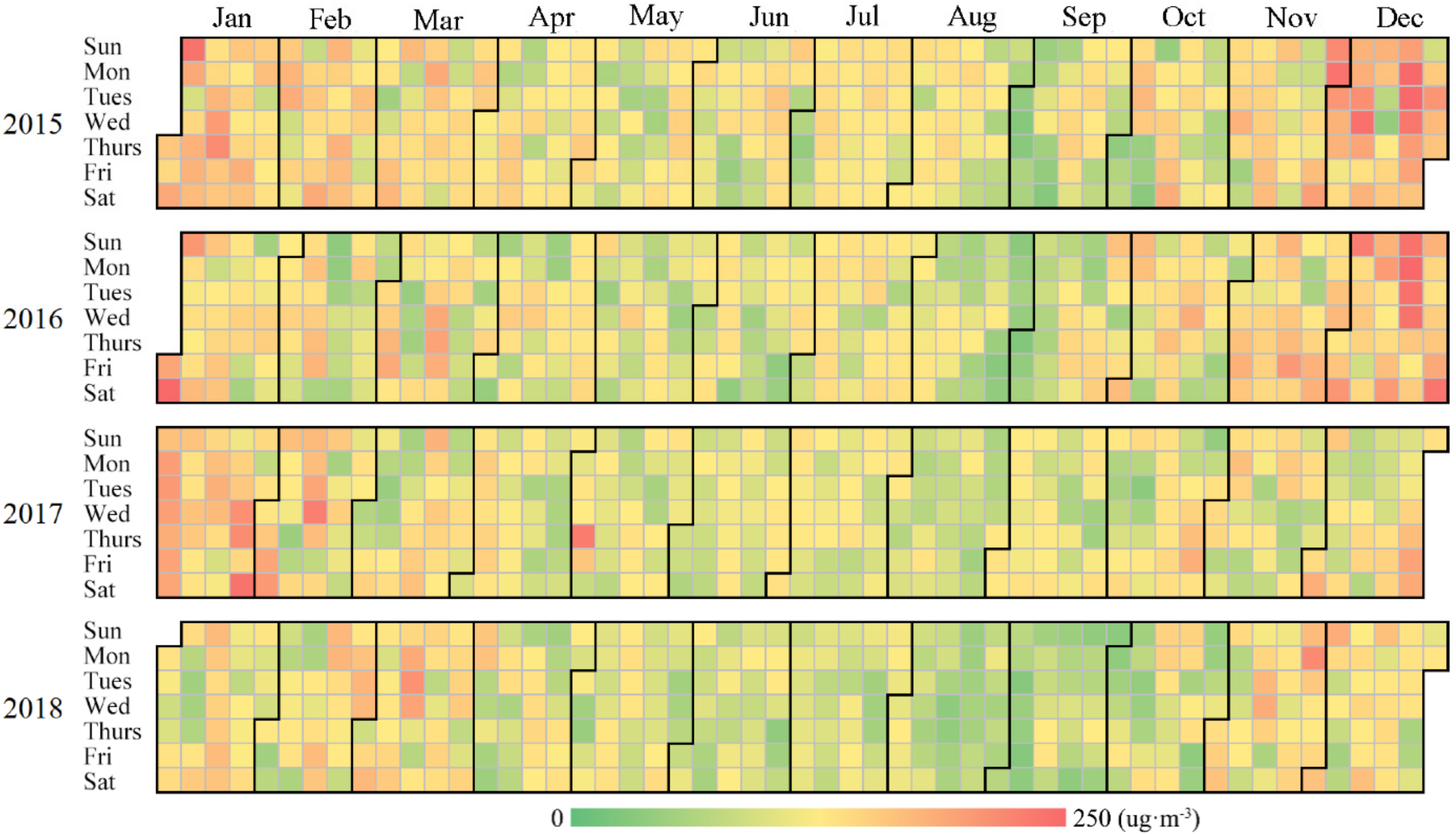
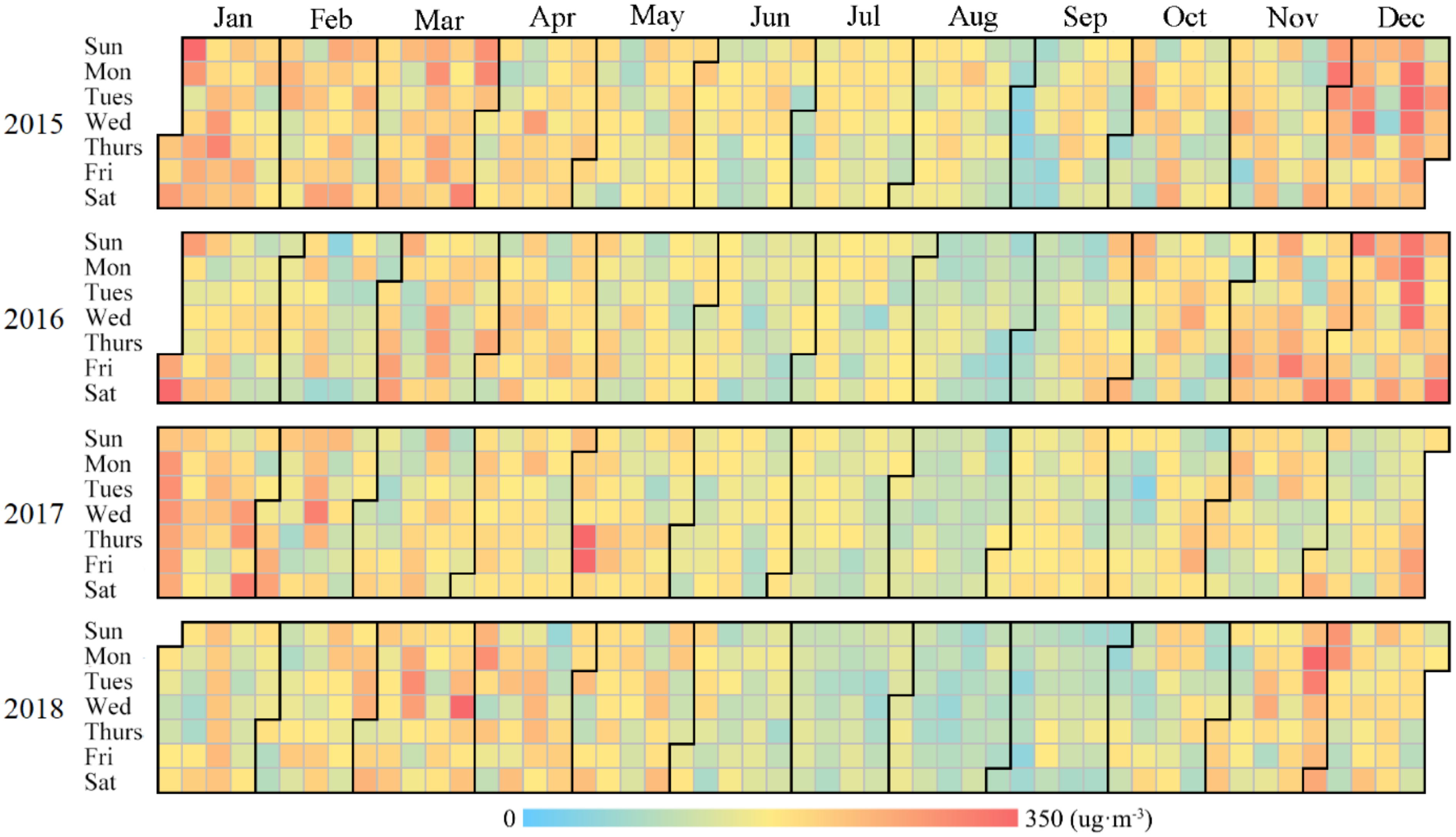
3.1. Temporal and Spatial Distribution Analysis of PM Concentration
3.2. Analysis of Environmental Elements
3.2.1. Meteorological Factors
3.2.2. Vegetation Factors
- (1)
- Forestland and grassland area
- (2)
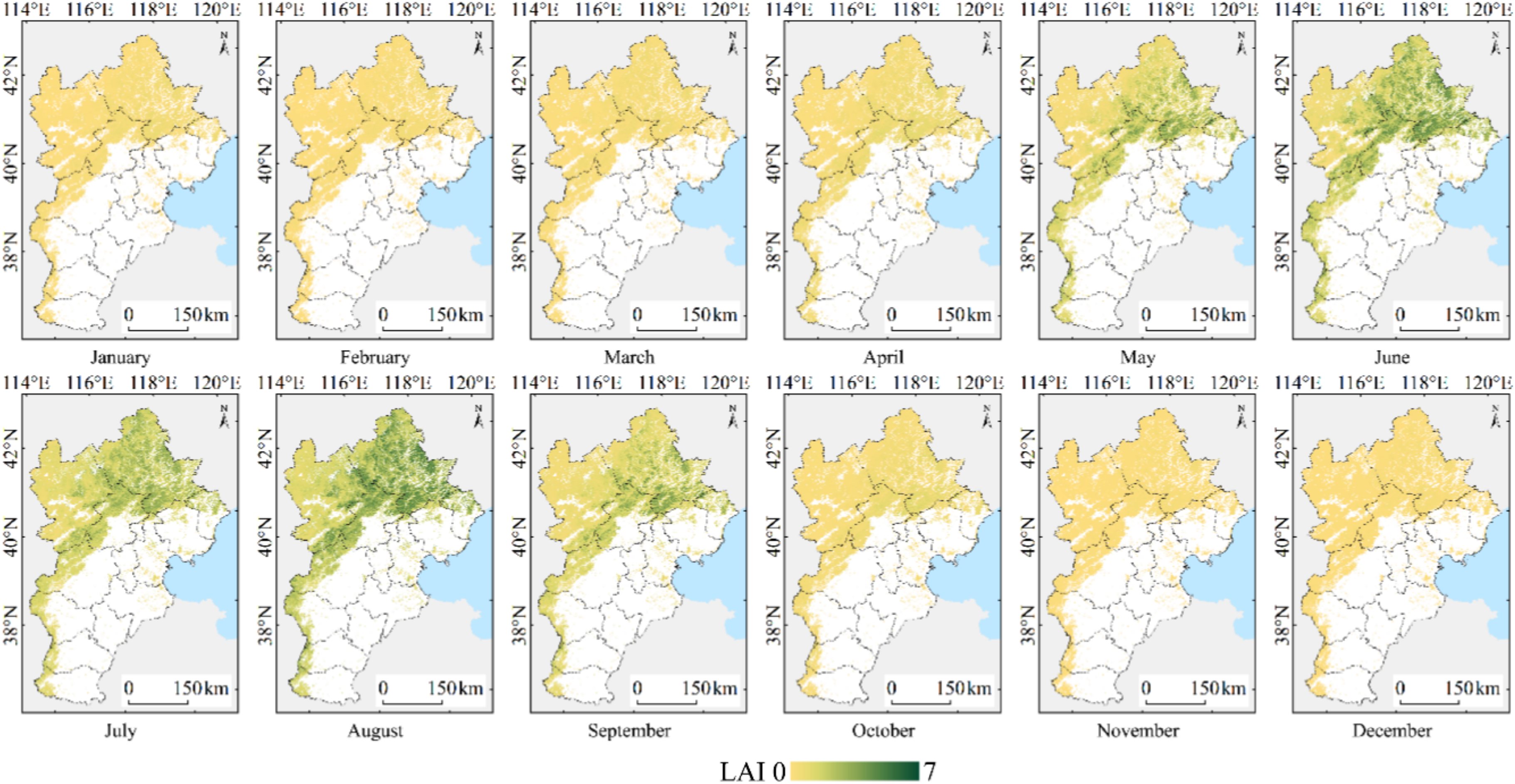
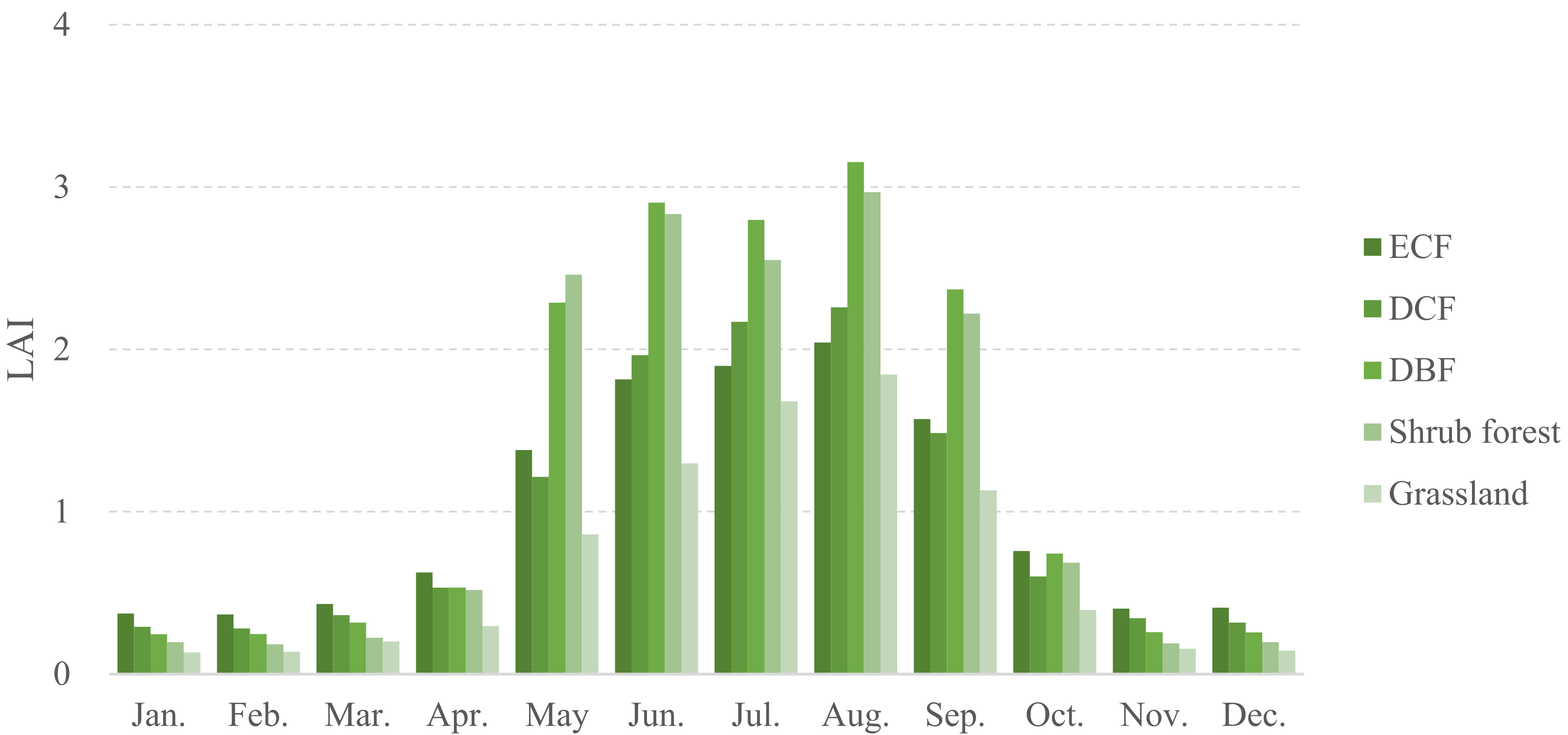
- LAI
3.3. Analysis of the Total Scale of Cities
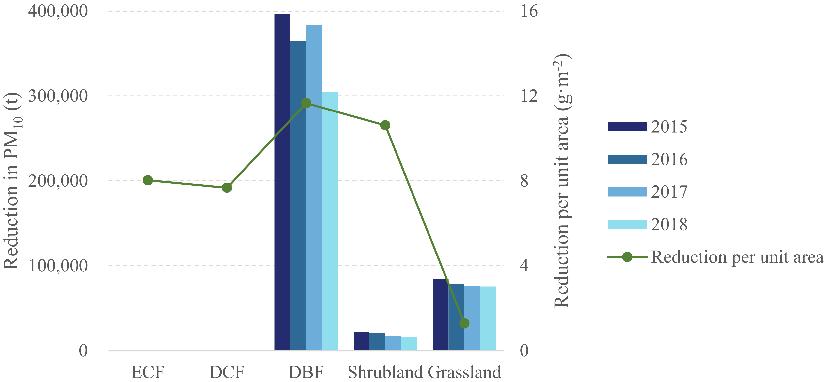
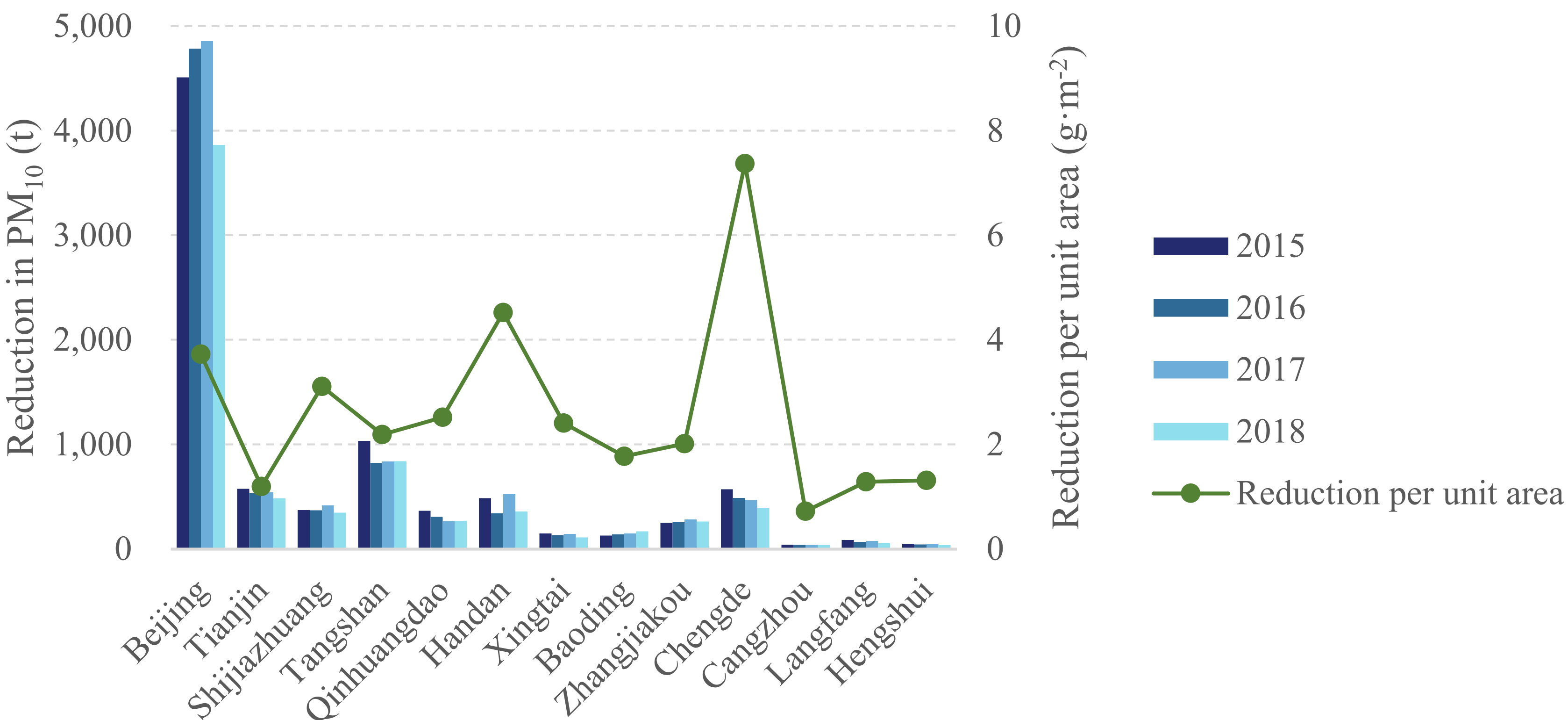
3.3.1. Reduction Effect of Vegetation Factors on PM10
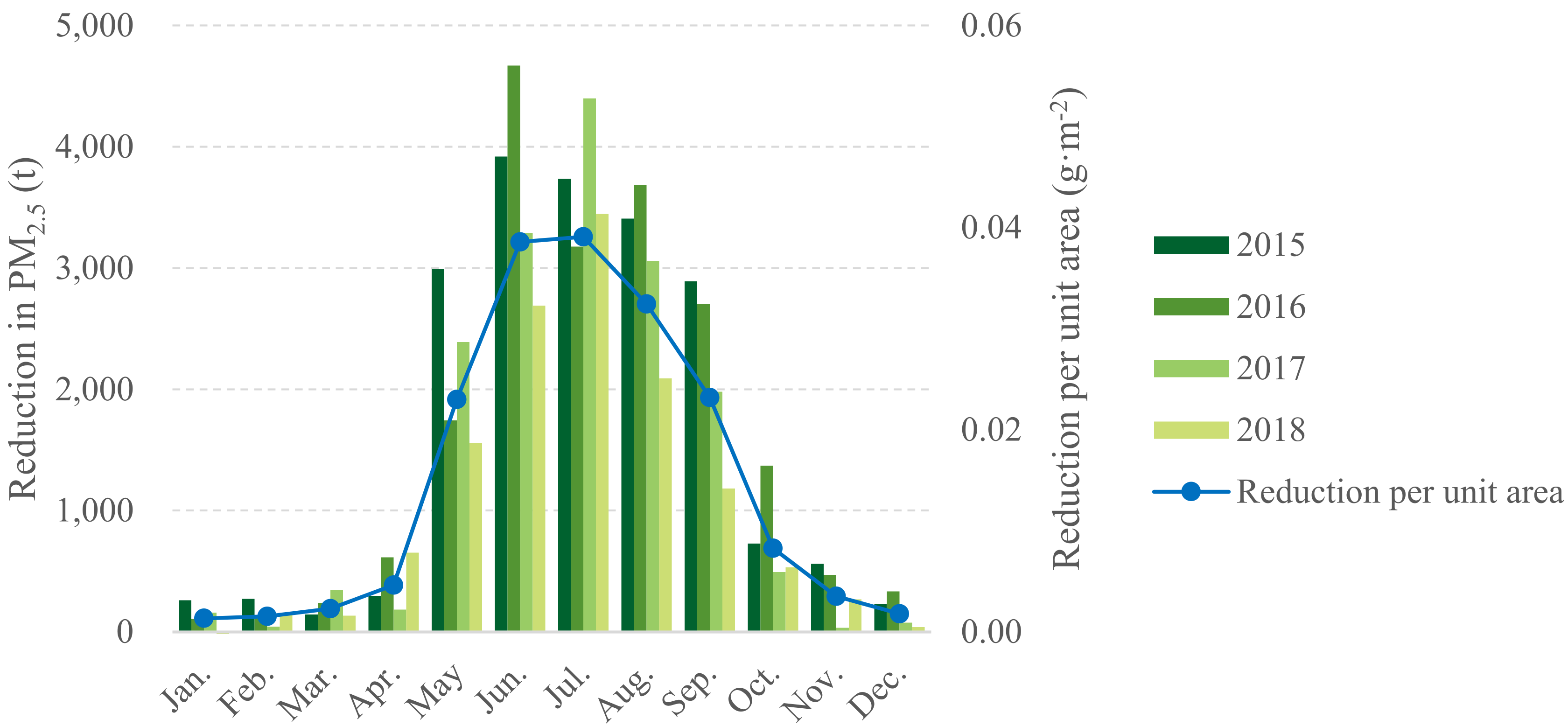
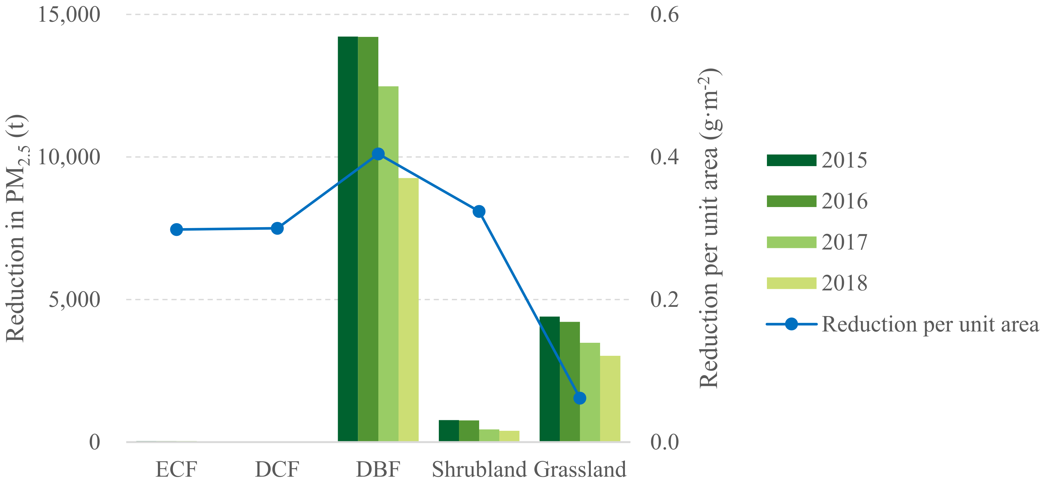
3.3.2. Reduction Effect of Vegetation Factors on PM2.5
3.4. Analysis on the Scale of the Built-Up Area
3.4.1. Reduction Effect of Vegetation Factors on PM10
3.4.2. Reduction Effect of Vegetation Factors on PM2.5
4. Discussion
4.1. Comparisons with Other Studies
4.2. Error Analysis
5. Conclusions
- (1)
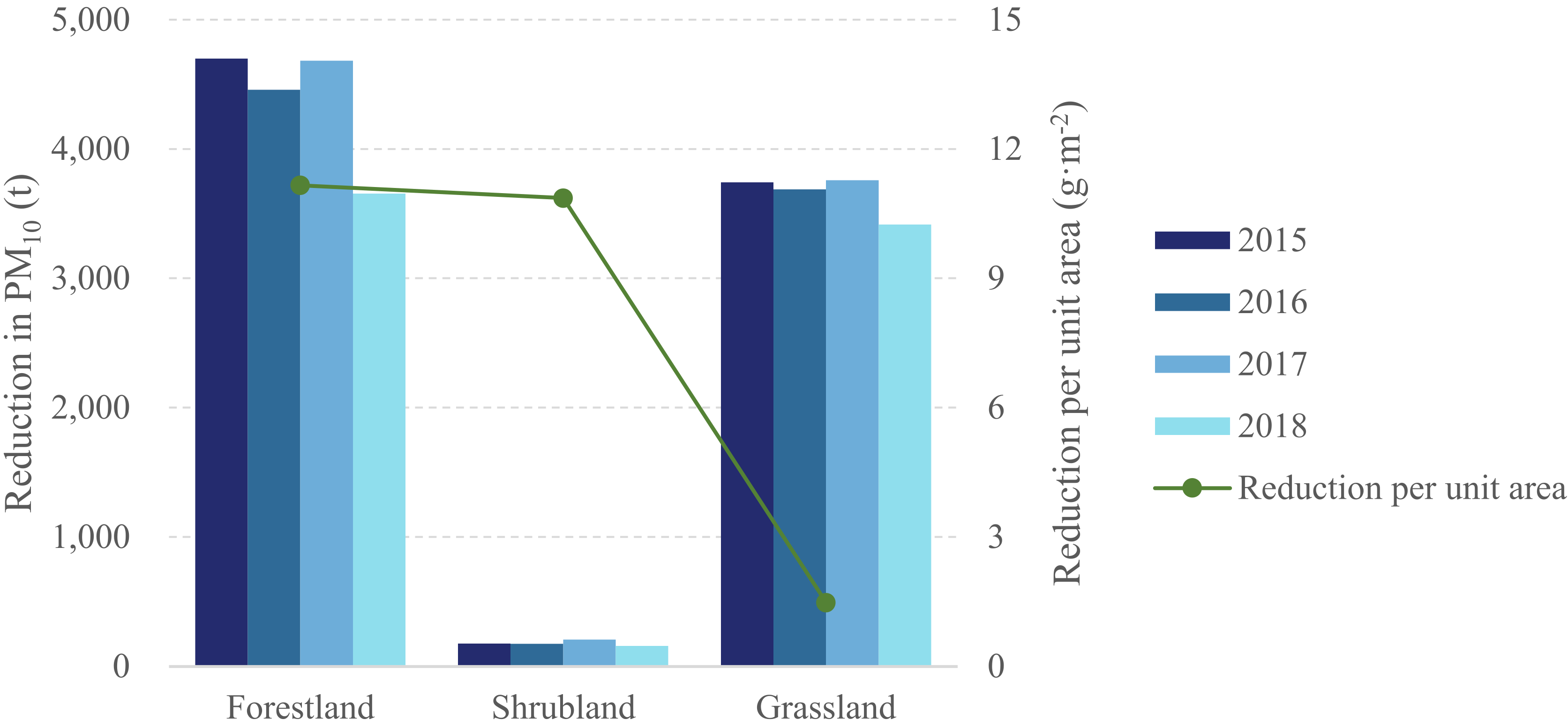
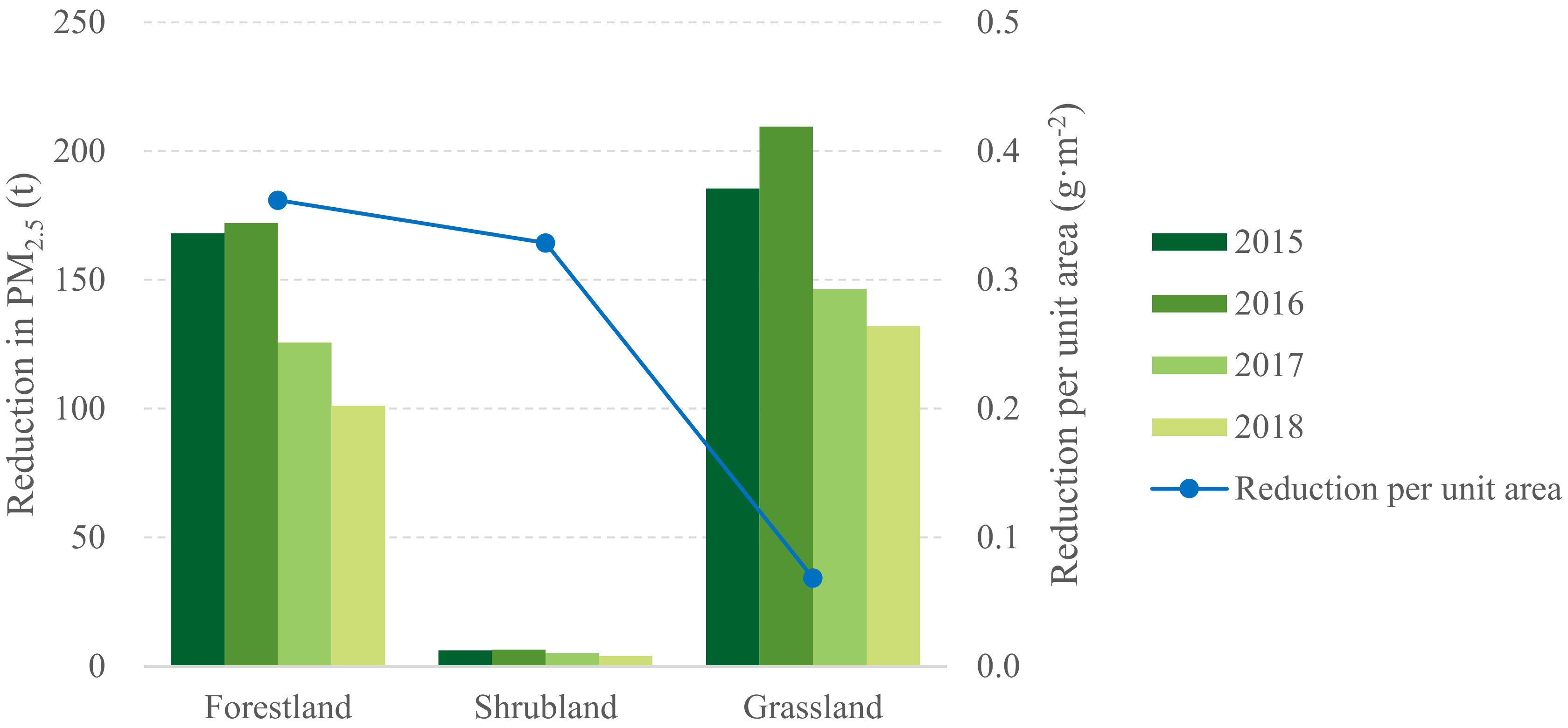
- The reduction in PM10 by vegetation was approximately 30 times that of PM2.5. However, the reduction in PM2.5 by vegetation should not be ignored because PM2.5 has a stronger correlation with human production and living activities. The total amounts of PM10 reduced by forestland and grassland in the BTH area were 505,200 t, 465,500 t, 477,200 t and 396,500 t in 2015, 2016, 2017 and 2018, respectively, and the concentrations of PM10 were reduced by 0.454 μg·m−3, 0.417 μg·m−3, 0.429 μg·m−3 and 0.429 μg·m−3, respectively, per hour. The total amount of PM2.5 was reduced by 19,400 t, 19,200 t, 16,400 t and 12,700 t in 2015, 2016, 2017 and 2018, respectively, and the concentration of PM2.5 was reduced by 0.017 μg·m−3, 0.017 μg·m−3, 0.015 μg·m−3 and 0.011 μg−3 per hour, respectively.
- (2)
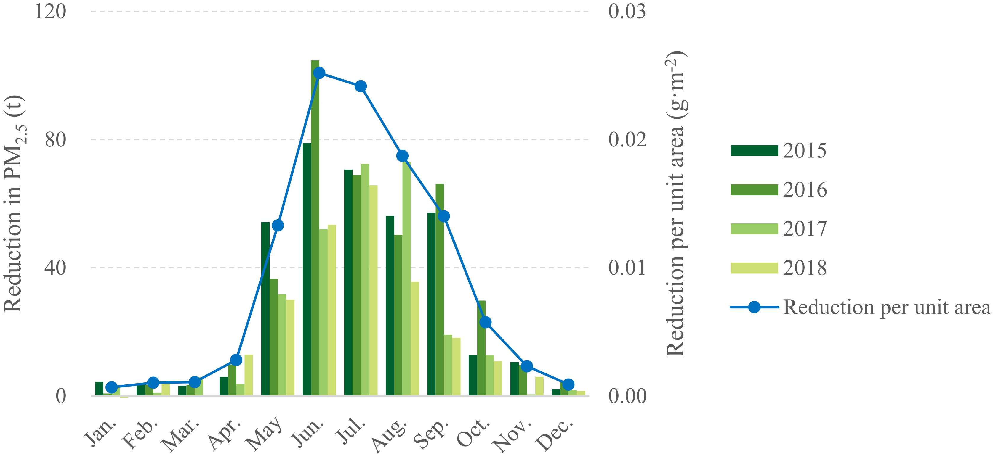
- The reduction amount, concentration reduction value and concentration improvement rate of vegetation for PM10 were significantly higher than those for PM2.5. However, because PM2.5 has a stronger correlation with human production and living activities, the reduction effect of vegetation on PM2.5 cannot be ignored. More than 80% of the reduction in annual yield was concentrated in May–September, and a large leaf area was the main reason for the largest yield reduction in the growing season. The efficiency of PM reduction in forestland was approximately five–seven times that in grassland, and DBF was the main driver of PM reduction in each forest. Reducing and controlling the concentration of PM by increasing the area and density of green space to create an environment suitable for dry sedimentation and giving full play to the functional effect of green space ecosystems are very important.
Author Contributions
Funding
Conflicts of Interest
References
- Churg, A.; Brauer, M.; del Carmen Avila-Casado, M.; Fortoul, T.I.; Wright, J.L. Chronic exposure to high levels of particulate air pollution and small airway remodeling. Environ. Health Perspect. 2003, 111, 714–718. [Google Scholar] [CrossRef] [PubMed] [Green Version]
- Hoek, G.; Krishnan, R.M.; Beelen, R.; Peters, A.; Ostro, B.; Brunekreef, B.; Kaufman, J.D. Long-term air pollution exposure and cardio-respiratory mortality: A review. Environ. Health 2013, 12, 43. [Google Scholar] [CrossRef] [PubMed] [Green Version]
- Cao, J. Major causes and control strategies of the PM2.5 pollution in China. Sci. Technol. Rev. 2016, 34, 74–80. [Google Scholar]
- Butlin, R.N.; Coote, A.T.; Devenish, M.; Hughes, I.S.C.; Hutchens, C.M.; Irwin, J.G.; Lloyd, G.O.; Massey, S.W.; Webb, A.H.; Yates, T.J.S. Preliminary results from the analysis of metal samples from the National Materials Exposure Programme (NMEP). Atmos. Environment. Part B. Urban Atmos. 1992, 26, 199–206. [Google Scholar] [CrossRef]
- Zhang, X.-Y. Aerosol over China and Their Climate Effect. Adv. Earth Sci. 2007, 22, 12–16. [Google Scholar]
- Lu, F.; Xu, D.; Cheng, Y.; Dong, S.; Guo, C.; Jiang, X.; Zheng, X. Systematic review and meta-analysis of the adverse health effects of ambient PM2.5 and PM10 pollution in the Chinese population. Environ. Research. Sect. A 2015, 136, 196–204. [Google Scholar] [CrossRef] [PubMed]
- Maleki, H.; Sorooshian, A.; Goudarzi, G.; Nikfal, A.; Baneshi, M.M. Temporal profile of PM10 and associated health effects in one of the most polluted cities of the world (Ahvaz, Iran) between 2009 and 2014. Aeolian Res. 2016, 22, 135–140. [Google Scholar] [CrossRef] [Green Version]
- Janssen, N.A.; Hoek, G.; Simic-Lawson, M.; Fischer, P.; Van Bree, L.; Ten Brink, H.; Cassee, F.R. Black carbon as an additional indicator of the adverse health effects of airborne particles compared with PM10 and PM2.5. Environ. Health Perspect. 2011, 119, 1691–1699. [Google Scholar] [CrossRef] [Green Version]
- Lou, C.; Liu, H.; Li, Y.; Li, Y. Research on the response of air particles (PM2.5, PM10) to landscape structure: A review. Acta Ecol. Sin. 2016, 36, 6719–6729. [Google Scholar]
- Nguyen, T.; Yu, X.; Zhang, Z.; Liu, M.; Liu, X. Relationship between types of urban forest and PM2.5 capture at three growth stages of leaves. J. Environ. Sci. 2015, 27, 33–41. [Google Scholar] [CrossRef] [PubMed]
- Tallis, M.; Taylor, G.; Sinnett, D.; Freer-Smith, P. Estimating the removal of atmospheric particulate pollution by the urban tree canopy of London, under current and future environments. Landsc. Urban Plan. 2011, 103, 129–138. [Google Scholar] [CrossRef]
- Yi, X.-Y.; Peng, Y.-H.; Liao, J.-Y.; Liu, Y.; Li, G.-F. A review of the relationship between forest vegetation and atmospheric particulate matter. Plant Sci. J. 2017, 35, 156–162. [Google Scholar]
- Xie, L.; Huang, F.; Gan, X.; Wen, X.; Huang, Y. Research progress on the purification effects of urban forest vegetation on atmospheric particulate pollution matter. For. Environ. Sci. 2017, 33, 96–103. [Google Scholar]
- Ma, K.; Yin, Z.; Zhang, Y. Advancement in the method and mechanism of the green space dust retention effect. Acta Ecol. Sin. 2018, 38, 391–400. [Google Scholar]
- Wu, H.; Yu, X.; Shi, C.; Zhang, Y.; Zhang, Z. Advances in the study of PM2.5 characteristic and the regulation of forests to PM2.5. Sci. Soil Water Conserv. 2012, 10, 116–122. [Google Scholar]
- Cao, H.; Yin, S.; Zhang, X.; Xiong, F.; Zhu, P.; Liu, C. Modeled PM2.5 removal by urban forest in Shanghai. J. Shanghai Jiaotong Univ. Agric. Sci. 2016, 34, 76–83. [Google Scholar]
- Xiao, Y.; Wang, S.; Li, N.; Xie, G.; Lu, C.; Zhang, B.; Zhang, C. Atmospheric PM2.5 removal by green spaces in Beijing. Resour. Sci. 2015, 37, 1149–1155. [Google Scholar]
- Nowak, D.J.; Hirabayashi, S.; Doyle, M.; McGovern, M.; Pasher, J. Air pollution removal by urban forests in Canada and its effect on air quality and human health. Urban For. Urban Green. 2018, 29, 40–48. [Google Scholar] [CrossRef]
- Nowak, D.J.; Crane, D.E.; Stevens, J.C. Air pollution removal by urban trees and shrubs in the United States. Urban For. Urban Green. 2006, 4, 115–123. [Google Scholar] [CrossRef]
- Al-Dousari, A.M.; Alsaleh, A.; Ahmed, M.; Misak, R.; William, T. Off-road vehicle tracks and grazing points in relation to soil compaction and land degradation. Earth Syst. Environ. 2019, 3, 471–482. [Google Scholar] [CrossRef]
- Abd El-Wahab, R.H.; Al-Rashed, A.R.; Al-Dousari, A. Influences of physiographic factors, vegetation patterns and human impacts on aeolian landforms in arid environment. Arid. Ecosyst. 2018, 8, 97–110. [Google Scholar] [CrossRef]
- Escobedo, F.J.; Nowak, D.J. Spatial heterogeneity and air pollution removal by an urban forest. Landsc. Urban Plan. 2009, 90, 102–110. [Google Scholar] [CrossRef]
- Vos, P.E.J.; Maiheu, B.; Vankerkom, J.; Janssen, S. Improving local air quality in cities: To tree or not to tree? Environ. Pollut. 2013, 183, 113–122. [Google Scholar] [CrossRef] [PubMed]
- Zhang, X.; Jiao, D.; Huang, T.; Zhagn, L.; Gao, H.; Zhao, Y.; Ma, J. Atmospheric removal of PM2.5 by man-made Three Northern Regions Shelter Forest in Northern China estimated using satellite retrieved PM2.5 concentration. Sci. Total Environ. 2017, 593–594, 713–721. [Google Scholar] [CrossRef] [PubMed]
- Al-Dousari, A.; Pye, K.; Alhazza, A.; Al-Shati, F.; Rajab, M. Nanosize inclusions as a fingerprint for aeolian sediments. J. Nanoparticle Res. 2020, 22, 94. [Google Scholar] [CrossRef]
- Al-Dousari, A.; Ibrahim, M.I.; Al-Dousari, N.; Ahmed, M.; Awadhi, S.A. Pollen in aeolian dust with relation to allergy and asthma in Kuwait. Aerobiologia 2018, 34, 325–336. [Google Scholar] [CrossRef]
- Nowak, D.J.; Crane, D.E. The Urban Forest Effects (UFORE) model: Quantifying urban forest structure and functions. Integr. Tools Proc. 2000, 212, 714–720. [Google Scholar]
- Chen, J.M.; Black, T.A. Defining leaf area index for non-flat leaves. Agric. For. Meteorol. 1992, 15, 421–429. [Google Scholar] [CrossRef]
- Gower, S.T.; Kucharik, C.J.; Norman, J.M. Direct and indirect estimation of leaf area index, fAPAR, and net primary production of terrestrial ecosystems. Remote Sens. Environ. 1999, 70, 29–51. [Google Scholar] [CrossRef]
- Lovett, G.M. Atmospheric deposition of nutrients and pollutants in North America: An ecological perspective. Ecol. Appl. 1994, 4, 630–650. [Google Scholar] [CrossRef]
- Zinke, P.J. Forest interception studies in the United States. In Forest Hydrology; Sopper, W.E., Lull, H.W., Eds.; Pergamon Press: Oxford, UK, 1967; pp. 137–161. [Google Scholar]
- Hirabayashi, S.; Kroll, C.N.; Nowak, D.J. i-Tree Eco Dry Deposition Model Descriptions. Available online: https://www.itreetools.org/documents/60/iTree_Eco_Dry_Deposition_Model_Descriptions.pdf (accessed on 27 February 2015).
- Tiwary, A.; Sinnett, D.; Peachey, C.; Chalabi, Z.; Vardoulakis, S.; Fletcher, T.; Leonardi, G.; Grundy, C.; Azapagic, A.; Hutchings, T.R. An integrated tool to assess the role of new planting in PM10 capture and the human health benefits: A case study in London. Environ. Pollut. 2009, 157, 2645–2653. [Google Scholar] [CrossRef] [Green Version]
- Baldocchi, D.D.; Hicks, B.B.; Camara, P. A canopy stomatal resistance model for gaseous deposition to vegetated surfaces. Atmos. Environ. 1987, 21, 91–101. [Google Scholar] [CrossRef]
- Yang, J.; Mcbride, J.; Zhou, J.; Sun, Z. The urban forest in Beijing and its role in air pollution reduction. Urban For. Urban Green. 2005, 3, 65–78. [Google Scholar] [CrossRef]
- Nowak, D.J.; Crane, D.E.; Stevens, J.C.; Hoehn, R.E.; Walton, J.T.; Bond, J. A ground-based method of assessing urban forest structure and ecosystem services. Arboric. Urban For. 2008, 34, 347–358. [Google Scholar] [CrossRef]
- Freer-Smith, P.H.; Elkhatib, A.A.; Taylor, G. Capture of particulate pollution by trees: A comparison of species typical of semi-arid areas (ficus nitida and eucalyptus globulus) with European and North American Species. Water Air Soil Pollut. 2004, 155, 173–187. [Google Scholar] [CrossRef]
- Beckett, K.P.; Freer-Smith, P.H.; Taylor, G. Particulate pollution capture by urban trees: Effect of species and windspeed. Glob. Change Biol. 2000, 6, 995–1003. [Google Scholar] [CrossRef]
- Pullman, M.R. Conifer PM2.5 Deposition and Re-Suspension in Wind and Rain Events; Cornell University: New York, NY, USA, 2009. [Google Scholar]
- Shreffler, J.H. Factors affecting dry deposition of SO2 on forests and grasslands. Atmos. Environ. 1978, 12, 1497–1503. [Google Scholar] [CrossRef]
- Escobedo, F.J.; Wagner, J.E.; Nowak, D.J.; Maza, C.L.D.L.; Rodriguez, M.; Crane, D.E. Analyzing the cost effectiveness of Santiago, Chile’s policy of using urban forests to improve air quality. J. Environ. Manag. 2008, 86, 148–157. [Google Scholar] [CrossRef] [PubMed]
- Fowler, D.; Skiba, U.; Nemitz, E.; Choubedar, F.; Branford, D.; Donovan, R.; Rowland, P. Measuring aerosol and heavy metal deposition on urban woodland and grass using inventories of 210 Pb and metal concentrations in soil. Water Air Soil Pollut. Focus 2004, 4, 483–499. [Google Scholar] [CrossRef]
- Mcdonald, A.G.; Bealey, W.J.; Fowler, D.; Dragosits, U.; Skiba, U.; Smith, R.I.; Donovan, R.G.; Brett, H.E.; Hewitt, C.N.; Nemitz, E. Quantifying the effect of urban tree planting on concentrations and depositions of PM in two UK conurbations. Atmos. Environ. 2007, 41, 8455–8467. [Google Scholar] [CrossRef]
- Zhao, H.; Che, H.; Xia, X.; Wang, Y.; Wang, H.; Wang, P.; Ma, Y.; Yang, H.; Liu, Y.; Wang, Y.; et al. Climatology of mixing layer height in China based on multi-year meteorological data from 2000 to 2013. Atmos. Environ. 2019, 213, 90–103. [Google Scholar] [CrossRef]
- Wang, J.; Endreny, T.A.; Nowak, D.J. Mechanistic simulation of tree effects in an urban water balance model. Jawra J. Am. Water Resour. Assoc. 2010, 44, 75–85. [Google Scholar] [CrossRef]
- Jiang, L.; Zhou, H.; Lai, Z.; Bai, L.; Chen, Z. Analysis of spatio-temporal characteristic of PM2.5 concentrations of Chinese cities: 2015–2017. Acta Sci. Circumstantiae 2018, 38, 3816–3825. [Google Scholar]
- Nowak, D.J.; Hirabayashi, S.; Bodine, A.; Hoehn, R. Modeled PM2.5 removal by trees in ten U.S. cities and associated health effects. Environ. Pollut. 2013, 178, 395–402. [Google Scholar] [CrossRef] [PubMed]
- Conte, M.; Donateo, A.; Contini, D. Characterisation of particle size distributions and corresponding size-segregated turbulent fluxes simultaneously with CO2 exchange in an urban area. Sci. Total Environ. 2018, 622–623, 1067–1078. [Google Scholar] [CrossRef] [PubMed]
- Casquero-Vera, J.A.; Lyamani, H.; Titos, G.; Moreira, G.d.A.; Benavent-Oltra, J.A.; Conte, M.; Continid, D.; Järvie, L.; Olmo-Reyes, F.J.; Alados-Arboledas, L. Aerosol number fluxes and concentrations over a southern European urban area. Atmos. Environ. 2022, 269, 118849. [Google Scholar] [CrossRef]
- Scott, K.I.; McPherson, E.G.; Simpson, J.R. Air pollutant uptake by Sacramento’s urban forest. J. Arboric. 1998, 24, 224–234. [Google Scholar]
- Chang, Y.M. Analysis of PM2.5 Removal by New Plantations in the Beijing Plain Area; Beijing Forestry University: Beijing, China, 2015. [Google Scholar]
- Chen, L.; Liu, C.-L.; Pan, T.; Chen, C.-C.; Li, Z.; Wang, H.-H.; Pei, S.; Sun, L. Assessment of the effect of PM2.5 reduction by plain afforestation project in Beijing based on dry deposition model. Chin. J. Ecol. 2014, 33, 2897–2904. [Google Scholar]


| Varieties of Trees | Wind Speed (m·s−1) | ||||
|---|---|---|---|---|---|
| 1 | 3 | 6 | 8.5 a | 10 | |
| Quercus petraea [37] | 0.00831 | 0.01757 | 0.03134 | ||
| Alnus glutinosa [37] | 0.00125 | 0.00173 | 0.00798 | ||
| Fraxinus excelsior [37] | 0.00178 | 0.00383 | 0.00725 | ||
| Acer pseudoplatanus [37] | 0.00042 | 0.00197 | 0.00344 | ||
| Psuedotsuga menziesii [37] | 0.01269 | 0.01604 | 0.0604 | ||
| Eucalyptus globulus [37] | 0.00018 | 0.00029 | 0.00082 | ||
| Ficus nitida [37] | 0.00041 | 0.00098 | 0.00234 | ||
| Pinus nigra [38] | 0.0013 | 0.0115 | 0.1924 | 0.2805 | |
| Cupressocyparis × leylandii [38] | 0.0008 | 0.0076 | 0.0824 | 0.122 | |
| Acer campestre [38] | 0.0003 | 0.0008 | 0.0046 | 0.0057 | |
| Sorbus intermedia [38] | 0.0004 | 0.0039 | 0.0182 | 0.0211 | |
| Populus deltoides [38] | 0.0003 | 0.0012 | 0.0105 | 0.0118 | |
| Pinus strobus [39] | 0.000108 | ||||
| Tsuga canadensis [39] | 0.000193 | ||||
| Tsuga japonica [39] | 0.000058 | ||||
| Maximum value for Picea abies b [39] | 0.000189 | ||||
| Minimum value for Picea abies b [39] | 0.00038 | ||||
| Median | 0.0003 | 0.00152 | 0.00197 | 0.00924 | 0.0211 |
| Standard error | 0.00012 | 0.00133 | 0.00281 | 0.0161 | 0.05257 |
| Maximum c | 0.00057 | 0.00442 | 0.00862 | 0.05063 | 0.14542 |
| Minimum d | 0.00006 | 0.00018 | 0.00029 | 0.00082 | 0.0057 |
| Wind Speed (m·s−1) | Deposition Velocity (m·s−1) | Resuspension Rate [39] |
|---|---|---|
| 1 | 0.0003 | 0.015 |
| 2 | 0.0009 | 0.030 |
| 3 | 0.0015 | 0.045 |
| 4 | 0.0017 | 0.060 |
| 5 | 0.0019 | 0.075 |
| 6 | 0.0020 | 0.090 |
| 7 | 0.0056 | 0.100 |
| 8 | 0.0092 | 0.110 |
| 9 | 0.0092 | 0.120 |
| 10 | 0.0211 | 0.130 |
| 11 | 0.0211 | 0.160 |
| 12 | 0.0211 | 0.200 |
| Time | ECF | DCF | DBF | Shrubland | Grassland |
|---|---|---|---|---|---|
| 2015 | 107 | 29 | 29,358 | 2089 | 63,452 |
| 2016 | 108 | 30 | 30,907 | 1992 | 61,000 |
| 2017 | 110 | 31 | 32,621 | 1429 | 59,661 |
| 2018 | 114 | 29 | 31,944 | 1686 | 61,164 |
Publisher’s Note: MDPI stays neutral with regard to jurisdictional claims in published maps and institutional affiliations. |
© 2022 by the authors. Licensee MDPI, Basel, Switzerland. This article is an open access article distributed under the terms and conditions of the Creative Commons Attribution (CC BY) license (https://creativecommons.org/licenses/by/4.0/).
Share and Cite
Zhai, H.; Yao, J.; Wang, G.; Tang, X. Study of the Effect of Vegetation on Reducing Atmospheric Pollution Particles. Remote Sens. 2022, 14, 1255. https://doi.org/10.3390/rs14051255
Zhai H, Yao J, Wang G, Tang X. Study of the Effect of Vegetation on Reducing Atmospheric Pollution Particles. Remote Sensing. 2022; 14(5):1255. https://doi.org/10.3390/rs14051255
Chicago/Turabian StyleZhai, Haoran, Jiaqi Yao, Guanghui Wang, and Xinming Tang. 2022. "Study of the Effect of Vegetation on Reducing Atmospheric Pollution Particles" Remote Sensing 14, no. 5: 1255. https://doi.org/10.3390/rs14051255
APA StyleZhai, H., Yao, J., Wang, G., & Tang, X. (2022). Study of the Effect of Vegetation on Reducing Atmospheric Pollution Particles. Remote Sensing, 14(5), 1255. https://doi.org/10.3390/rs14051255