BM3D Denoising for a Cluster-Analysis-Based Multibaseline InSAR Phase-Unwrapping Method

Abstract

Multibaseline (MB) phase unwrapping (PU) is a key processing technique in MB interferometric synthetic aperture radar (InSAR). As one of the most popular methods, the cluster analysis (CA)-based MBPU method often suffers from the problem of low noise robustness. Therefore, the block-matching and 3D filtering (BM3D) algorithm, one of the most effective filtering methods for image denoising, is applied to improve the performance of the method. Five different filtering strategies for applying BM3D are proposed in the paper: interferogram filtering (IFF), intercept filtering (ICF), cluster number filtering (CNF), unwrapped phase filtering (UPF), and simultaneous filtering (STF). In particular, while keeping the general structure of BM3D, four different similarity measures are defined for interferograms, intercepts, clusters, and unwrapped phases to accommodate the special characteristics of different filtering objects. Experiments on synthesized and real InSAR datasets prove their feasibility and effectiveness, and the experiment results show that (1) the PU accuracy and robustness of the CA-based MBPU method can be greatly improved by adding BM3D denoising; (2) simultaneous filtering of interferograms, intercepts, cluster numbers, and unwrapped phases works best, but with the worst time complexity; (3) when filtering is performed for only one object of the CA-based MBPU method, the filtering effect of CNF and UPF is better than that of IFF and ICF; and (4), considering the three indicators of PUSR, NRSE, and time consumption, CNF and UPF should be the best choices.

1. Introduction

Interferometric synthetic aperture radar (InSAR) can acquire multiple synthetic radar images of an observed region and measure their interferometric phases to obtain the corresponding terrain height information (such as a digital elevation model, DEM) or deformation information [1,2,3,4,5]. However, the measured interferometric phase is wrapped into the principal value interval, which is modulo 2$\pi$. In order to obtain the correct absolute interferometric phase, phase unwrapping (PU) must be performed [6]. The accuracy of the target elevation is directly related to the PU accuracy, so PU has always been a key processing step in InSAR applications.

Researchers first proposed single-baseline phase-unwrapping (SBPU) methods to reconstruct the unwrapped phase, and several representative works are introduced in [7,8,9]. However, the traditional SBPU method must assume that the actual phase jump between adjacent pixels is less than $\pi$ to ensure the uniqueness of the solution, which is called the phase continuity assumption. When the phase jump between adjacent pixels of the observed terrain is greater than $\pi$, the accurate phase-unwrapping results cannot be obtained using the SBPU technique.

Therefore, multibaseline phase-unwrapping (MBPU) algorithms are further proposed to overcome the limitation of SBPU. According to [6], there are two main categories of MBPU methods: parametric-based methods and nonparametric-based methods. The parametric-based methods construct a statistical framework according to the probability density function of the interferometric phase and regard the elevation or elevation difference as the parameters to be estimated. In [10], a PU method for reconstructing highly discontinuous ground elevation profiles using ML technology was proposed. In [11], an improved technique based on ML estimation was proposed to reconstruct the elevation information. In this method, a multifrequency independent phase dataset obtained by nonoverlapping band-pass filtering the interferometric SAR raw data pair was used, and the unknown surface was approximated by the local plane assumption. In [12], a maximum a posteriori (MAP) estimation method based on multifrequency interferometry and a Markov random fields (MRFs) model was proposed. In [13], the MAP estimation method was improved based on the total variation model and graph-cut-based optimization algorithms. In [14], an enhanced MBPU method by combining an unscented Kalman filter with an enhanced joint phase gradient estimator was proposed. In [15], an extended Kalman filter (EKF)-based MBPU approach, which has the ability of handling phase discontinuities, was proposed. In [16], a nonlocal denoising method based on patch similarities and total-variation regularization was proposed to realize resolution-preserving denoising and robust MBPU for DEM reconstruction.

The nonparametric-based methods do not need the probability density function of the interferometric phase and directly use multiple interferograms with different baseline lengths to reconstruct the absolute phase. In [17], H. Yu et al. proposed a two-stage programming approach (TSPA), which transplants the SBPU framework to MBPU. In [18,19], two refined TSPA methods were presented. The first method is abbreviated as LPM-TSPA [18], and it improves the performance of stage one of the TSPA by approximating the terrain surface to a local plane, which allows more interferometric phase information to be used to estimate the ambiguity number gradient. The second refined TSPA-based MBPU method proposed in [19] uses an unscented Kalman filter (UKF) to improve the performance of stage two of the TSPA. As one of the most popular methods, the cluster analysis (CA)-based MBPU method has also been widely studied. In [20], the ambiguity vectors corresponding to each pixel are solved according to the closed-form robust Chinese remainder theorem (CRT), and then clustering is performed according to the ambiguity vectors. In order to improve the noise robustness of the conventional CRT-based MBPU method, a fast CA algorithm was proposed in [21], which clusters pixels with the same ambiguity vector into a group according to the recognizable mathematical pattern, i.e., intercept information, and the ambiguity vectors of all pixels in the same cluster can be estimated through the group-by-group clustering center information. In [22], a refined CA-based method was proposed by linearly combining multiple InSAR interferograms with different baseline lengths, which makes the new combined interferogram have a larger ambiguity interval. In [23], the recognizable mathematical patterns were expanded into row, line, and intercept, which further improves the noise robustness of the CA-based method. In [24], a new closed-form robust CA-based MBPU and filtering algorithm (MBPUF) was proposed to improve the efficiency, height reconstruction accuracy, and noise robustness of the CA-based MBPU method.

In addition, the application of deep learning in PU is becoming more and more extensive. In [25], deep learning was applied to the CA algorithm, and an unsupervised deep convolutional neural network named CANet was proposed. In [26], a novel deep convolutional neural network (DCNN), abbreviated as PGNet, was proposed for estimating the phase gradient information instead of phase continuity assumptions. In [27,28], by reformulating the definition of the problem of directly obtaining the continuous original phase as the wrap count obtained on each pixel through semantic segmentation, a novel framework called PhaseNet that uses a deep, fully convolutional neural network to unwrap the phase network was proposed. In [29], a comprehensive overview of InSAR phase unwrapping based on artificial intelligence was provided, which reviews the SBPU and MBPU methods based on artificial intelligence. In addition to PU, deep learning also has many applications in SAR and InSAR, and readers can refer to [30,31,32,33,34].

As a representative MBPU method, the CA-based MBPU method has the following problems: (1) it has poor noise robustness and is sensitive to phase noise, i.e., small phase noises may cause large unwrapping errors [23]; (2) when the intercepts of the cluster with fewer pixels and the cluster with more pixels are very close, the two clusters will be merged into one cluster due to the presence of phase noise, resulting in wrong clustering results [23]; and (3) it does not have phase-filtering capability [24]. In order to solve the above problems, this paper introduces filtering techniques into the CA-based MBPU method. In SAR and InSAR applications, traditional methods mainly use filtering techniques for interferograms [35,36,37,38] or SAR images [39,40].

However, in this paper, we consider the application of the current state-of-the-art BM3D technology to the four objects involved in the CA-based MBPU method: interferogram, intercept, cluster number, and unwrapped phase. The main advantages of the BM3D technology are as follows [41]: (1) it has achieved the most advanced denoising performance in terms of peak signal-to-noise ratio and subjective visual quality; (2) it can be adapted to various noise models by modifying the coefficient variance calculation in the basic and Wiener parts of the algorithm; and (3) it preserves relatively complete information about the structure of the original image. Therefore, five different filtering strategies for applying BM3D are proposed: interferogram filtering (IFF), intercept filtering (ICF), cluster number filtering (CNF), unwrapped phase filtering (UPF), and simultaneous filtering (STF). In particular, while keeping the general structure of BM3D, four different similarity measures are defined for interferograms, intercepts, clusters, and unwrapped phases to accommodate the special characteristics of different filtering objects.

The rest of this paper is organized as follows. First, Section 2 reviews the principle of the CA-based MBPU method and points out the shortcomings of this method. Section 3 briefly reviews the structure of the BM3D algorithm. Section 4 introduces the application of the BM3D algorithm to the CA-based MBPU method. In Section 5, experiments on simulated and real data are introduced to prove the effectiveness and feasibility of the proposed method, and the results are discussed. Finally, the conclusions are given in Section 6.

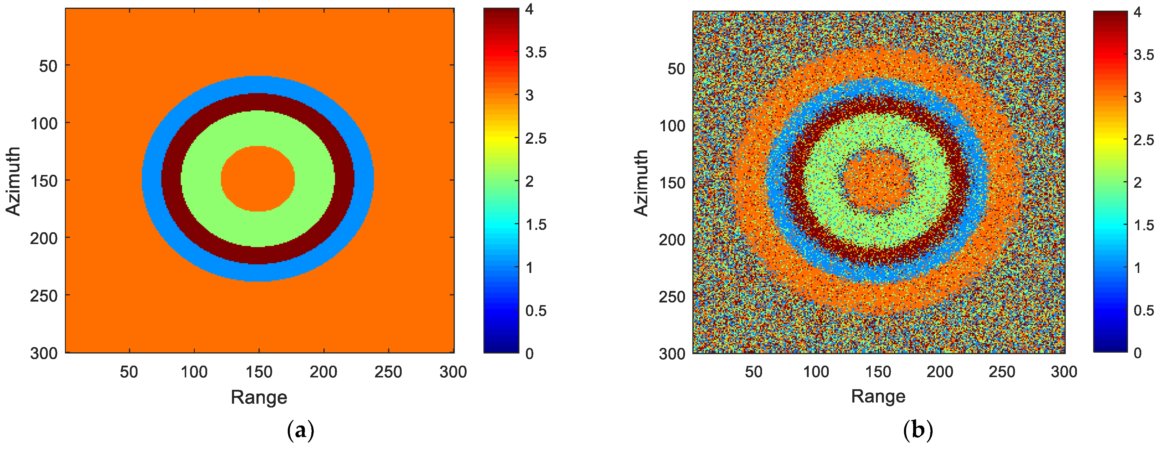
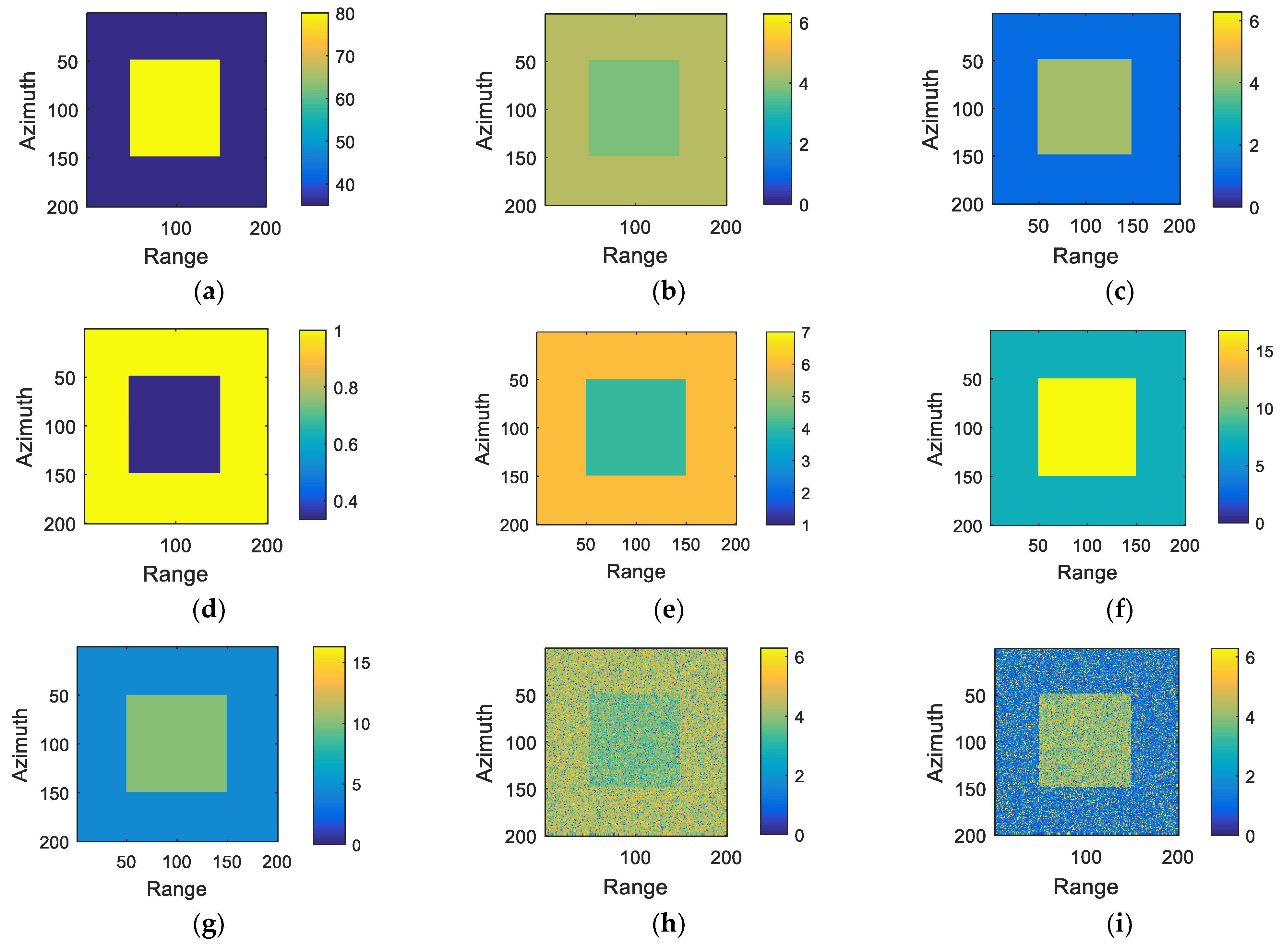
2. Basic Principle of the CA-Based MBPU Method

For an InSAR system, the terrain height can be obtained from the unwrapped phase and other system parameters [18]:

$$h\left(p\right)=\frac{\lambda ·r\left(p\right)·sin{\theta }_o}{4\pi ·B_i}·{\psi }_i\left(p\right)$$

(1)

where $h\left(p\right)$ is the terrain height of the p-th pixel, $\lambda$ is the working wavelength of the InSAR system, $r(p)$ represents the slant range of the p-th pixel for the main channel, ${\theta }_o$ is the look angle, $B_i$ is the length of the orthogonal baseline for the i-th interferogram, and ${\psi }_i\left(p\right)$ is the flattened absolute interferometric phase of the p-th pixel for the i-th interferogram. The measured phase of the target obtained by the system, namely the wrapped phase, can be expressed by [7]:

$${\phi }_i\left(p\right)={\psi }_i\left(p\right)-2\pi ·k_i\left(p\right)$$

(2)

where ${\phi }_i\left(p\right)$ is the wrapped phase of the p-th pixel of the i-th interferogram (from 0 to 2π in this paper) and $k_i\left(p\right)$ is the unknown integer ambiguity of the p-th pixel of the i-th interferogram. It can be seen from (2) that the purpose of PU is to find the correct value of $k_i\left(p\right)$ to obtain the correct unwrapped phase ${\psi }_i\left(p\right)$.

For simplicity, only the case of two different baselines is considered for now. Then, the following equation can be obtained according to (1) and (2):

$$\frac{B_1}{B_2}=\frac{{\phi }_1\left(p\right)+2\pi ·k_1\left(p\right)}{{\phi }_2\left(p\right)+2\pi ·k_2\left(p\right)}$$

(3)

i.e.,

$$k_2\left(p\right)=\frac{B_2}{B_1}{k}_1\left(p\right)+\frac{B_2·{\phi }_1\left(p\right)-B_1·{\phi }_2\left(p\right)}{2\pi ·B_1}$$

(4)

It can be seen from (4) that the information of each pixel is reflected by a linear equation.

Because $B_1$ and $B_2$ are constants, the slope of the straight line is also a constant, while the intercept varies with ${\phi }_1\left(p\right)$ and ${\phi }_2\left(p\right)$. According to [21], the term ambiguity vector $\left[k_1\left(p\right),k_2\left(p\right)\right]$ is defined as the ambiguity numbers corresponding to a pixel in two different interferograms. Additionally, a cluster is defined as a set of pixels with the same ambiguity vector. Obviously, the intercepts of the pixels in a cluster are the same since their corresponding straight lines pass through the same integer point $\left[k_1,k_2\right]$ and with the same slope: $B_2/B_1$. Therefore, the cluster to which a pixel belongs can be determined by its corresponding intercept information.

Through the above analysis, the main steps of the CA-based MBPU method can be summarized as follows: (1) the intercepts of all pixels are calculated according to the input interferograms; (2) the cluster to which each pixel belongs is obtained by using the CA algorithm; (3) the cluster ambiguity vectors of each cluster are calculated according to CRT and the intercept of each cluster’s centerline; and (4) the final unwrapped phases of each pixel are acquired by the cluster ambiguity vectors and wrapped phases. Although the CA-based MBPU methods can meet the requirements of PU to a certain extent, the poor noise robustness makes the algorithm prone to produce erroneous clustering results. It should be noted that when the clustering is finished, a natural number is assigned to each cluster, which is called the cluster number. A cluster number is a natural number we artificially set for each cluster, and the purpose is to number the clustering results. Different cluster numbers represent different clusters. Therefore, we can use Figure 1 to show the influence of noise on the clustering results.

Figure 1a shows the clustering results under noiseless conditions, where different colors represent different clusters. It can be seen from Figure 1a that there are obviously four different clusters. Figure 1b is the noisy clustering result generated by the CA algorithm, and there are some wrong clustering results due to the existence of noise. In addition, although the CA algorithm improves the noise robustness and reduces the time complexity to a certain extent when the cluster with fewer pixels is very close to the cluster with more pixels, these two clusters will be merged into one cluster due to the presence of phase noise [23], resulting in erroneous clustering results. Therefore, the BM3D algorithm can be applied to the CA-based MBPU method to improve PU accuracy. According to the main steps of the CA-based MBPU method, BM3D can be applied to the following four objects: (1) the interferograms; (2) the intercepts; (3) the cluster numbers; and (4) the unwrapped phases.

3. BM3D Algorithm and Similarity Measures Improvement

In this section, we first review the basic processing procedure and then define four similarity measures for the four different objects to be filtered in this paper: interferograms, intercepts, clusters, and unwrapped phases.

3.1. BM3D Algorithm

The basic flow chart of the BM3D algorithm is shown in Figure 2. According to [30], the BM3D algorithm was originally proposed for Gaussian white noise, which combines nonlocal methods with wavelet domain shrinkage and Wiener filtering. Then, the main steps of the BM3D algorithm can be described as follows [30].

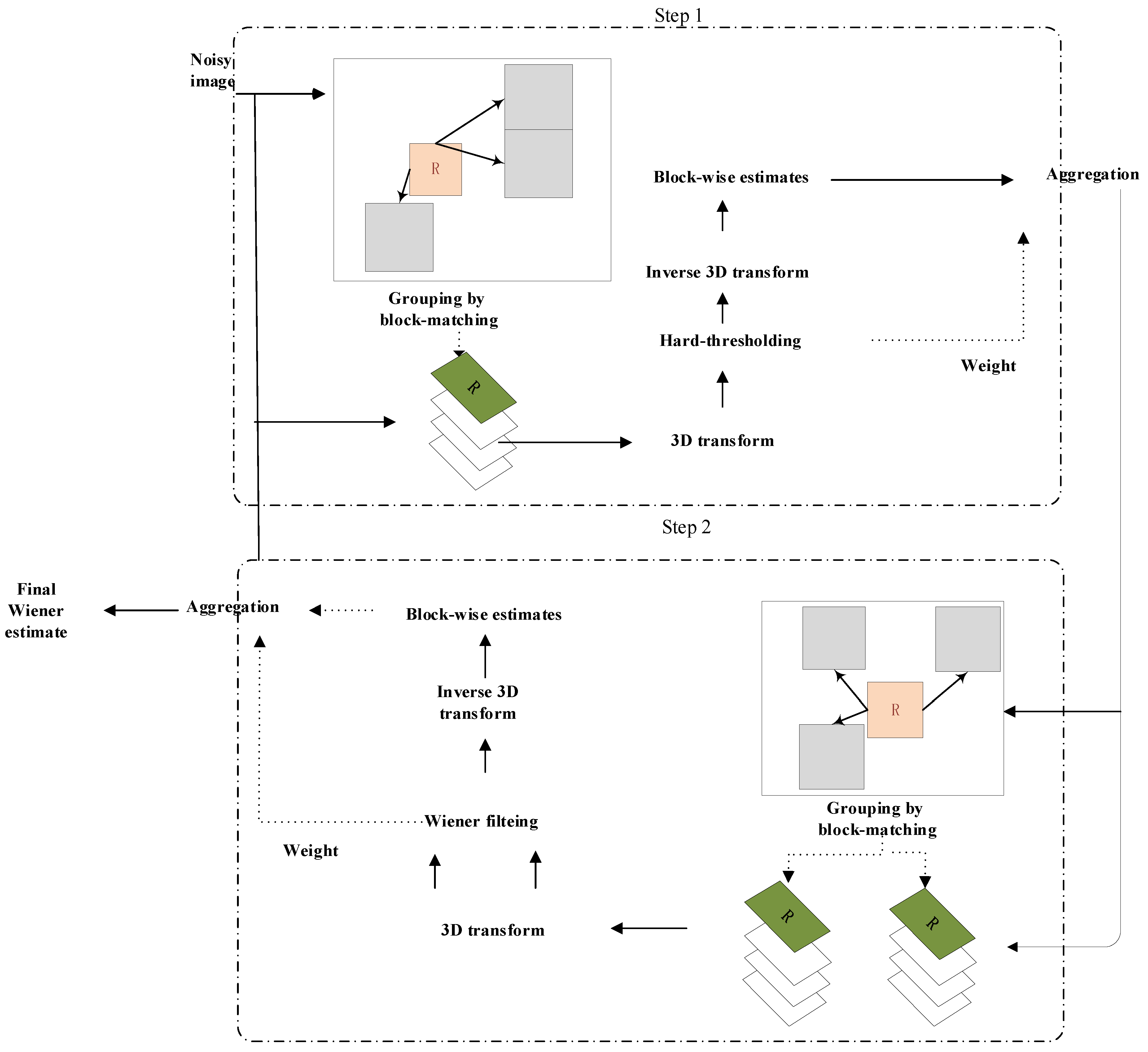
3.1.1. The First Stage, Basic Estimate

(1)

Block-matching grouping: Find blocks that are similar to the reference block and named as similar blocks, and the similarity is determined by calculating the predefined distance between the reference block and the block to be matched. Then, the similar blocks are stacked into a 3D array according to the similarity, which is called a 3D group.

(2)

Collaborative hard thresholding: Perform 3D transformation processing on the 3D groups, attenuate noise through hard thresholding, and then use 3D inverse transformation to obtain the estimated values of the 2D similar blocks.

(3)

Aggregation: Since there are often overlapping parts between the blocks, the result is the same pixel often being contained in several different blocks. Therefore, the pixel value of each pixel is repeatedly estimated, and a weighted average of these multiple estimates is needed to obtain the basic estimate for each block.

3.1.2. The Second Stage, Final Estimate (the Basic Estimate Is Used as the Input)

(1)

Block-matching grouping: Find the position of similar blocks by means of block-matching in basic estimation. Block-matching grouping consists of two parts, which can obtain two 3D groups, one from the noise image and the other from the basic estimated image.

(2)

Collaborative Wiener filtering: Apply 3D transformation to the above two 3D groups, use the 3D group in the basic estimation as the energy spectrum of the real signal, use the energy spectrum to perform collaborative Wiener filtering on the noise image, and finally, the processed data are inversely transformed and returned to the original position of the similar block to obtain the final estimated value.

(3)

Aggregation: Because the blocks obtained after grouping and filtering may overlap each other, weighted average processing on pixels with multiple estimated values is performed to obtain the final estimation.

3.2. Similarity Measures Improvement

In the block-matching grouping of the original BM3D algorithm, the similarity between two blocks is usually expressed by the inverse of some distance measured between them [30]. The smaller the distance is, the more similar the two blocks are. Since there are four different processing objects involved in the CA-based MBPU method, interferograms, intercepts, cluster numbers, and unwrapping phases, four different similarity measures are defined to accommodate the special characteristics of different filtering objects.

For the interferogram, the similarity of two pixels can be measured by the cosine value of their wrapped phase difference:

$$S({\phi }_1, {\phi }_2)=\frac{1+\cos ({\phi }_1-{\phi }_2)}{2}$$

(5)

where ${\phi }_1$ and ${\phi }_2$ represent the wrapped phases corresponding to two different pixels, respectively.

For the intercept, the similarity of two pixels is measured by the following formula:

$$S(b_1,b_2)=1-\frac{|b_1-b_2|}{\underset{1<p<n}{\max }(b_p)-\underset{1<p<n}{\min }(b_p)}$$

(6)

where $b_1$ and $b_2$ represent the intercepts of two different pixels, $\underset{1<p<n}{\max }(b_p)$ represents the largest intercept value among all the pixels, and $\underset{1<p<n}{\min }(b_p)$ represents the smallest intercept value among all the pixels.

For the cluster, the greater the difference between two cluster numbers, the greater the difference between the two pixels, so the similarity of the two pixels can be measured by:

$$S(m_1,m_2)=1-\frac{|m_1-m_2|}{\underset{1<p<n}{\max }(m_p)-\underset{1<p<n}{\min }(m_p)}$$

(7)

where $m_1$ and $m_2$ represent the cluster numbers of two different pixels, $\underset{1<p<n}{\max }(m_p)$ represents the largest cluster number among all the pixels, and $\underset{1<p<n}{\min }(m_p)$ represents the smallest cluster number among all the pixels.

For the unwrapped phase, the similarity can be measured by:

$$S({\psi }_1,{\psi }_2)=1-\frac{|{\psi }_1-{\psi }_2|}{\underset{1<p<n}{\max }({\psi }_p)-\underset{1<p<n}{\min }({\psi }_p)}$$

(8)

where ${\psi }_1$ and ${\psi }_2$ represent the unwrapped phases of two different pixels, $\underset{1<p<n}{\max }({\psi }_p)$ represents the largest unwrapped phase among all the pixels, and $\underset{1<p<n}{\min }({\psi }_p)$ represents the smallest unwrapped phase among all the pixels.

According to the definitions of Equations (5)–(8), the closer the value of S is to one, the stronger the similarity of the two pixels; on the contrary, the closer the value of S is to zero, the weaker the similarity of the two pixels.

4. BM3D Denoising for the CA-Based MBPU Method

Considering that it can perform denoising well and retain some original details of an image, the BM3D algorithm is applied to the CA-based MBPU method.

According to the main steps of the CA-based MBPU method described in Section 2, the BM3D algorithm is applied to the following four objects separately or simultaneously: (1) the wrapped phases, i.e., interferogram; (2) the intercepts; (3) the clustering results, i.e., cluster numbers; and (4) the unwrapped phases. There can be five different filtering strategies in total, and the corresponding basic flow charts are shown in Figure 3. Among them, the first four filtering strategies filter only one object, while the fifth filtering strategy filters all four objects at the same time. Moreover, all the five filtering strategies contain four main steps: data preprocessing, BM3D denoising, denormalization, and post-processing. In the following, we will describe these four main steps for applying the BM3D algorithm to the CA-based MBPU method in detail.

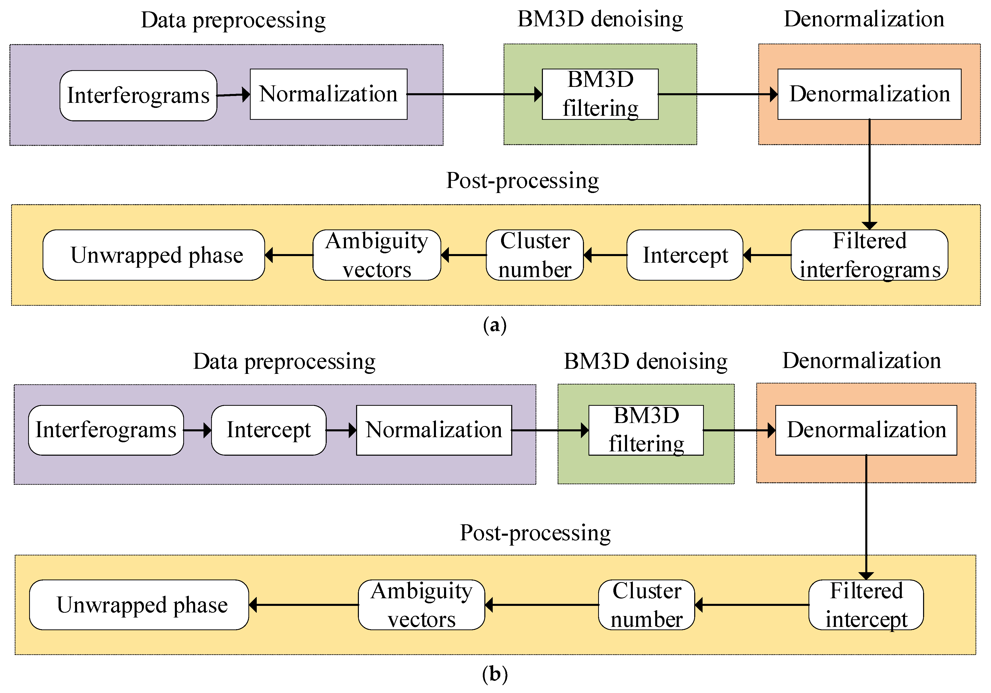
4.1. Data Preprocessing

The interferogram, intercept, cluster number, and unwrapped phase datasets to be filtered are first obtained according to the CA-based MBPU methods.

In order to uniformly use BM3D in the four objects of the CA-based MBPU methods, they need to be normalized, and the value range of these inputs should be changed to zero–one. Therefore, the normalization of these four objects can be implemented using the following four equations:

$${\phi }_{norm}(p)=\frac{\phi (p)}{2\pi }$$

(9)

$$b_{norm}(p)=\frac{b(p)-\underset{1<s<n}{\min }(b(p))}{\underset{1<s<n}{\max }(b(p))-\underset{1<s<n}{\min }(b(p))}$$

(10)

$$m_{norm}(p)=\frac{m(p)}{M}$$

(11)

$${\psi }_{norm}(p)=\frac{\psi (p)-\underset{1<s<n}{\min }(\psi (p))}{\underset{1<s<n}{\max }(\psi (p))-\underset{1<s<n}{\min }(\psi (p))}$$

(12)

where ${\phi }_{norm}(p)$ represents the normalized wrapped phase of pixel $p$, $b_{norm}(p)$ represents the normalized intercept of pixel $p$, $\underset{1<p<n}{\max }(b(p))$ represents the maximum intercept, $\underset{1<p<n}{\min }(b(p))$ represents the minimum intercept, $m_{norm}(p)$ represents the normalized cluster number of pixel $p$, $M$ represents the total number of clusters, ${\psi }_{norm}(p)$ represents the normalized unwrapped phase of pixel $p$, $\underset{1<p<n}{\max }(\psi (p))$ represents the maximum unwrapped phase, and $\underset{1<p<n}{\min }(\psi (p))$ represents the minimum unwrapped phase.

4.2. BM3D Denoising

The BM3D algorithm absorbs the processing idea of nonlocal filtering in the NL-means algorithm. In the filtering process, it further uses the information of block groups in the whole image. While keeping the general structure of BM3D, four different similarity measures are defined in Equations (5)–(8) for the four different processing objects involved in the CA-based MBPU method to accommodate the special characteristics of different filtering objects: interferograms, intercepts, cluster numbers and unwrapping phases. Moreover, five different filtering strategies for applying BM3D are proposed: interferogram filtering (IFF), intercept filtering (ICF), cluster number filtering (CNF), unwrapped phase filtering (UPF), and simultaneous filtering (STF).

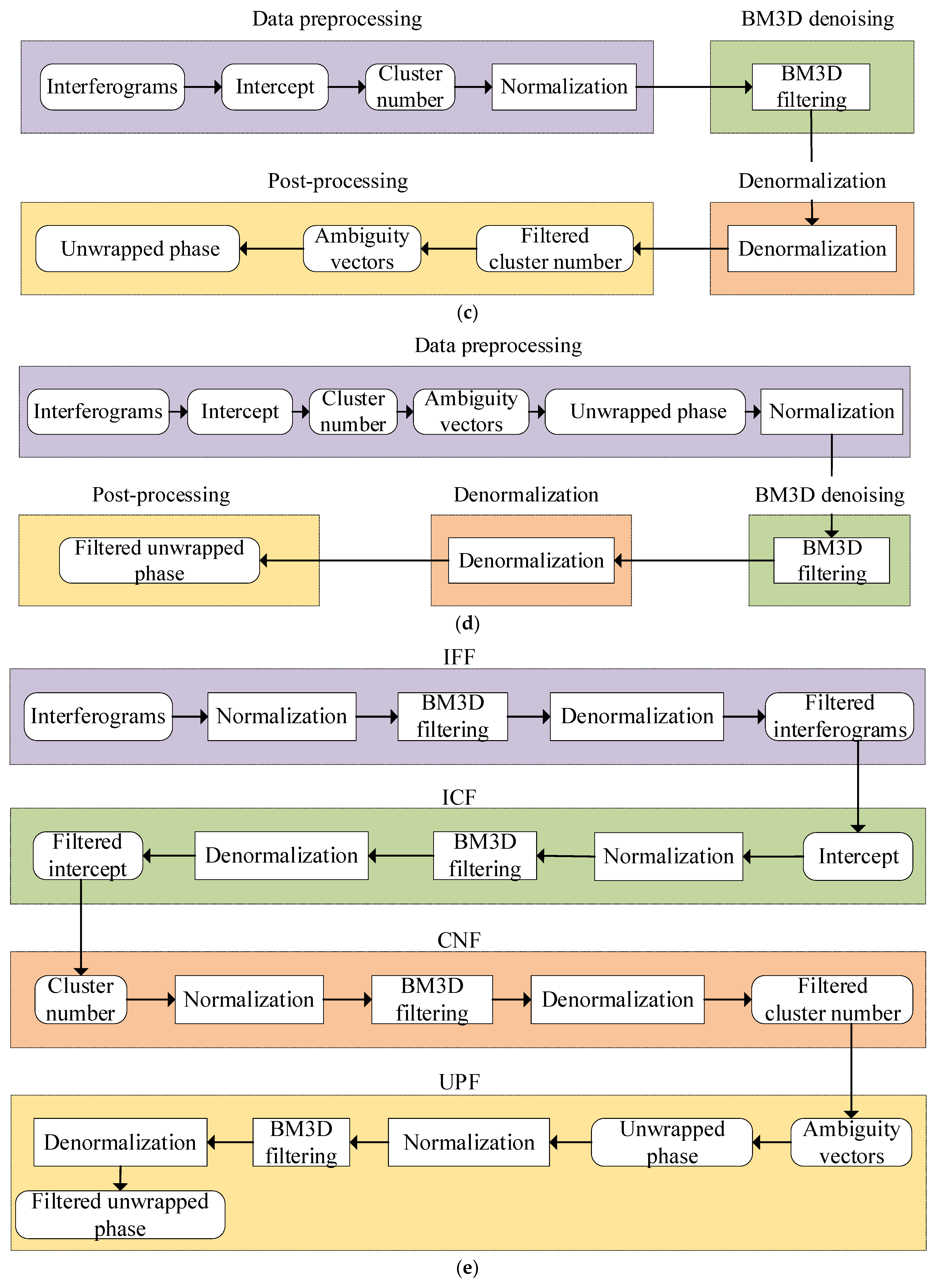
4.2.1. Interferogram Filtering (IFF)

Please refer to Figure 3a. In this method, the noisy interferogram is filtered directly by BM3D and the other steps are essentially unchanged. The wrapped phases are damaged due to the presence of noise, so filtering is performed on them. The noise interferogram is used as the input noise image of the BM3D algorithm to obtain the filtered wrapped phase ${\phi }_{filtered}(p)$, and then the filtered interferogram is used for the following other steps. This method is abbreviated as the IFF method.

4.2.2. Intercept Filtering (ICF)

Please refer to Figure 3b. Since the CA-based MBPU methods use the intercept as a clustering index, when they are contaminated by noise, the clustering results will be affected. Therefore, the intercepts contaminated by noise can be filtered using BM3D to obtain the filtered intercept $b_{filtered}(p)$, and then the filtered intercept is used for subsequent processing. This method is referred to as the ICF method in this paper.

4.2.3. Cluster Number Filtering (CNF)

Please refer to Figure 3c. Due to the presence of noise, errors will occur on the cluster numbers. Therefore, BM3D can be used after the clustering is completed. The cluster number distribution map is used as the input noise image of the BM3D algorithm, and the filtered cluster numbers $m_{filtered}(p)$ are used for the following other steps. This method is abbreviated as the CNF method in this paper.

4.2.4. Unwrapped Phase Filtering (UPF)

Please refer to Figure 3d. After the CA algorithm is completed, the unwrapped phase is restored. Due to the presence of noise, the obtained unwrapped phase contains errors. Therefore, BM3D can be used on the unwrapped phase, and the unwrapped phase is used as the input of the BM3D algorithm. Additionally, the filtered unwrapped phase ${\psi }_{filtered}(p)$ is obtained at last. This method is abbreviated as the UPF method in this paper.

4.2.5. Simultaneous Filtering (STF)

Please refer to Figure 3e. In fact, BM3D can be used to filter the interferogram, the intercept, the cluster number, and the unwrapped phase at the same time, so the best filtering results should be obtained. This method is abbreviated as the STF method in this paper.

4.3. Denormalization

After filtering, the obtained interferogram, intercept, cluster number, and unwrapped phase are, respectively, denormalized so that the subsequent clustering can be processed normally and the correct unwrapped phase can be obtained, that is, processed according to the following four equations:

$${\phi }_{final}(p)={\phi }_{filtered}(p)·2\pi$$

(13)

$$b_{final}(p)=b_{filtered}(p)·(\underset{1<p<n}{\max }(b(p))-\underset{1<p<n}{\min }(b(p)))+\underset{1<p<n}{\min }(b(p))$$

(14)

$$m_{final}(p)=m_{filtered}(p)·M$$

(15)

$${\psi }_{final}(p)={\psi }_{filtered}(p)·(\underset{1<p<n}{\max }(\psi (p))-\underset{1<p<n}{\min }(\psi (p)))+\underset{1<p<n}{\min }(\psi (p))$$

(16)

where ${\phi }_{final}(p)$ represents the final wrapped phase, $b_{final}(p)$ represents the final intercept, $m_{final}(p)$ represents the final cluster number, and ${\psi }_{final}(p)$ represents the final unwrapped phase.

4.4. Post-Processing

After being processed by the IFF method, the data obtained by filtering the interferogram need to be used in the subsequent steps of the CA-based MBPU methods to obtain the intercept, obtain the cluster number from the intercept, obtain the ambiguity number from the cluster number, and finally obtain the unwrapped phase. After being processed by the ICF method, the filtered intercept is used in the subsequent steps of the CA-based MBPU methods to obtain the cluster number, after which the ambiguity number is obtained from the cluster number and the unwrapped phase is finally obtained. After being processed by the CNF method, the obtained cluster number is used in the subsequent steps to obtain the ambiguity number and, finally the unwrapped phase. After being processed by the UPF method, the filtered unwrapped phase is obtained.

5. Results and Discussion

Experiments on synthesized and real InSAR datasets are shown in this section to verify the feasibility and effectiveness of the improved CA-based MBPU method by adding BM3D denoising.

The first experiment establishes a simple simulation scene, which shows smooth and discontinuous regions. The height of the scene was settled to 35 m and 80 m, respectively (the DEM is shown in Figure 4a), and the corresponding coherence coefficients were set to 0.5 and 0.6, respectively. The noiseless interferograms generated by simulation are shown in Figure 4b,c. There are only two clusters, and the corresponding cluster intercepts are 1 and 1/3, respectively. The real intercept distribution is shown in Figure 4d. The real cluster number distribution is shown in Figure 4e. The simulated noiseless unwrapped phase is shown in Figure 4f,g. The simulated noisy interferograms are shown in Figure 4h,i. As can be seen from the figure, the phase distribution becomes very ambiguous due to the addition of noise. The noisy intercept distribution is shown in Figure 4j. The noisy cluster number distribution obtained by the CA algorithm is shown in Figure 4k. The unwrapped phases obtained by the CA-based MBPU method are shown in Figure 4l,m.

Next, the BM3D algorithm was applied to the CA-based MBPU method to verify the effectiveness of the proposed method. First, the wrapped phases (interferograms) of long and short baselines with noise are taken as the inputs of BM3D and then filtered. The two filtered interferograms are shown in Figure 5a,b. They are used in the CA algorithm to obtain the cluster number distribution, as shown in Figure 5c. Second, BM3D is used to filter the noisy intercepts. The filtered intercept distribution map is shown in Figure 5d. Additionally, it is then applied to the CA algorithm to generate a cluster number distribution map, which is shown in Figure 5e. Third, the cluster numbers generated by clustering were filtered, as shown in Figure 5f. Fourth, the recovered unwrapped phases were filtered. The filtered unwrapped phases corresponding to the long and short baselines are shown in Figure 5g,h. Finally, BM3D is applied to the above four objects simultaneously, and the final unwrapped phases corresponding to the long and short baselines are shown in Figure 5i,j. It can be seen from the experimental results that the performance greatly improved after adding BM3D separately or simultaneously.

Then, the performance was quantitatively analyzed as follows. We used the phase unwrapping success rate (PUSR) and normalized reconstruction square error (NRSE) to check the accuracy of the results. First, the correctness of the unwrapped result was judged according to the correctness of the final obtained ambiguity vectors corresponding to all pixels. PUSR is defined as the percentage of pixels whose integer ambiguity is correctly restored in an interferogram to the total pixels. The higher the success rate of phase unwrapping, the higher the accuracy of representing the ambiguity number. When the accuracy of the ambiguity number is more correct, it shows that the accuracy of the clustering results is higher. Therefore, the success rate of phase unwrapping can be used to reflect the accuracy of the clustering results.

Table 1. PUSR of different filtering strategies.

Experiments	Filtering Strategies	Interferogram One	Interferogram Two
Experiment 1	No filtering	79.84%	79.26%
	IFF	97.78%	97.77%
	ICF	99.08%	99.06%
	CNF	99.85%	99.87%
	UPF	99.87%	99.89%
	STF	99.94%	99.94%
Experiment 2	No filtering	85.33%	84.21%
	IFF	88.02%	88.76%
	ICF	95.23%	95.37%
	CNF	98.99%	98.21%
	UPF	99.22%	98.87%
	STF	99.47%	99.33%
Experiment 3	No filtering	82.46%	81.22%
	IFF	89.21%	87.69%
	ICF	91.22%	91.21%
	CNF	95.41%	95.57%
	UPF	95.86%	95.87%
	STF	97.24%	98.41%

shows the PUSR of various methods in the experiment. It can be seen from Table 1 that the PUSR has been greatly improved after filtering. Obviously, it can be seen from Table 1 that the filtering effect of STF is the best because the STF filters all of the four objects. However, if only one object is filtered, the filtering effect of UPF and CNF is better than that of IFF and ICF. Second, the accuracy of the unwrapped result is judged through NRSE = ${\Vert \widehat{h}-h\Vert }^2/{\Vert h\Vert }^2$, used in [11,12,13,21,25], where $\widehat{h}$ is the height array estimated from the unwrapped phase array of an interferogram and $h$ is the reference height array.

As shown in

Table 2. Normalized reconstruction square error (NRSE).

Experiments	Filtering Strategies	NRSE
Experiment 1	No filtering	0.1812
	IFF	0.0342
	ICF	0.0221
	CNF	0.0089
	UPF	0.008
	STF	0.0045
Experiment 2	No filtering	0.2954
	IFF	0.2349
	ICF	0.1981
	CNF	0.1211
	UPF	0.1114
	STF	0.0974
Experiment 3	No filtering	0.3478
	IFF	0.3117
	ICF	0.2498
	CNF	0.1469
	UPF	0.1413
	STF	0.1347

, the NRSE of before filtering, IFF, ICF, CNF, UPF, and STF is 0.1812, 0.0342, 0.0221, 0.089, 0.0080 and 0.0045, respectively. Therefore, IFF, ICF, CNF, UPF, and STF can effectively improve the PU accuracy.

Table 3. Time consumption.

Experiments	Filtering Strategies	Time (s)
Experiment 1	IFF	0.6275
	ICF	0.6199
	CNF	0.6229
	UPF	0.6265
	STF	0.9598
Experiment 2	IFF	1.7787
	ICF	1.7474
	CNF	1.7977
	UPF	1.7545
	STF	2.0869
Experiment 3	IFF	2.7977
	ICF	2.8112
	CNF	2.7776
	UPF	2.7884
	STF	4.4857

shows the time consumption of the five filtering strategies. As can be seen from Table 2 and Table 3, if the time consumption is not considered, STF can better reduce the normalized square error and improve the PU accuracy than the other filtering strategies. However, the STF method has the highest time complexity. For the other four filtering strategies, they all have similar time complexity, but the filtering effect of UPF and CNF is better than that of IFF and ICF.

The second experiment tested the performance of different filtering strategies on a more realistic height profile. Figure 6a shows the reference DEM of Isolation Peak in Colorado, USA. The corresponding ambiguity heights were set to 32.1 m and 53.5 m, respectively. The simulated two noiseless interferograms are shown in Figure 6b,c. The real intercept distribution is shown in Figure 6d. The real cluster number distribution is shown in Figure 6e. The noiseless unwrapped phases for the long and short baselines are shown in Figure 6f,g. The noisy interferograms are shown in Figure 6h,i. As can be seen from the figure, the phase distribution became very ambiguous due to the noise. The noisy intercept distribution is shown in Figure 6j. The noisy cluster number distribution obtained by the CA algorithm is shown in Figure 6k. The noisy unwrapped phases for the long and short baselines obtained by the CA-based MBPU method are shown in Figure 6l,m.

Figure 7 shows the experimental results about Isolation Peak (CO, USA) with BM3D denoising. The two filtered interferograms of IFF are shown in Figure 7a,b, and the corresponding cluster number distribution is shown in Figure 7c. The filtered intercept distribution of ICF is shown in Figure 7d, and the corresponding cluster number distribution is shown in Figure 7e. The filtered cluster number distribution of CNF is shown in Figure 7f. The filtered unwrapped phases of UPF corresponding to the long and short baselines are shown in Figure 7g,h. The final unwrapped phases of STF corresponding to the long and short baselines are shown in Figure 7i,j. The relevant quantitative indexes for Experiment 2 are shown in Table 1, Table 2 and Table 3, respectively.

In the last experiment, a small-scale double-baseline TanDEM-X InSAR dataset with 736 × 191 pixels was tested by the proposed method. The scenario of this dataset is a mountainous area in Tongchuan City, Shaanxi Province, China. Figure 8a is the reference DEM obtained by the Space Shuttle Radar Topographic Mapping Mission (SRTM). The main parameters of the TanDEM-X InSAR dataset are shown in

Table 4. Parameters of the TanDEM-X InSAR dataset.

	Interferogram One		Interferogram Two
	TDX-1	TSX-1	TDX-2	TSX-2
Incidence angle	36.16°	36.07°	37.29°	37.05°
Acquisition date	2 April 2014		21 October 2012
Normal baseline	129.25 m		361.90 m
Range pixel spacing	5.45 m
Azimuth pixel spacing	8.15 m
Center latitude	35.28°N
Center longitude	109.27°E

. The two noisy TanDEM-X InSAR interferograms are shown in Figure 8b,c. The noisy intercept distribution is shown in Figure 8d. The noisy cluster number distribution obtained by the CA algorithm directly is shown in Figure 8e. The filtered interferograms of IFF are shown in Figure 8f,g. They are used to obtain the cluster number distribution. Figure 8h shows the cluster number distribution of IFF. The filtered intercept distribution of ICF is shown in Figure 8i, and the corresponding cluster number distribution of ICF is shown in Figure 8j. The filtered cluster number distribution of CNF is shown in Figure 8k. The filtered unwrapped phase of UPF corresponding to the long and short baselines are shown in Figure 8l,m. The unwrapped phases of STF corresponding to the long and short baselines are shown in Figure 8n,o. The relevant quantitative indexes for Experiment 3 are also shown in Table 1, Table 2 and Table 3, respectively. Obviously, the results of this experiment are in perfect agreement with the results of Experiment 1 and Experiment 2, thus strongly demonstrating the effectiveness and reliability of the filtering strategy proposed in this paper.

The three experimental results in Table 1, Table 2 and Table 3 demonstrate the effectiveness of the BM3D filtering strategies for the CA-based MBPU method on the simulated and real InSAR datasets.

6. Conclusions

MBPU is one of the key steps of InSAR processing. In order to improve the PU accuracy and the robustness of the CA-based MBPU method, five different filtering strategies for applying BM3D are proposed: interferogram filtering (IFF), intercept filtering (ICF), cluster number filtering (CNF), unwrapped phase filtering (UPF), and simultaneous filtering (STF). In particular, while keeping the general structure of BM3D, four different similarity measures are defined for interferograms, intercepts, clusters, and unwrapped phases to accommodate the special characteristics of different filtering objects. Experiments on simulated and real InSAR data prove the effectiveness and feasibility, and the experimental results show that (1) the PU accuracy and robustness of the CA-based MBPU method can be greatly improved by adding BM3D denoising; (2) simultaneous filtering of interferograms, intercepts, cluster numbers, and unwrapped phases works best, but with the worst time complexity; (3) when filtering is performed for only one object of the CA-based MBPU method, the filtering effect of CNF and UPF is better than that of IFF and ICF; and (4) considering the three indicators of PUSR, NRSE, and time consumption, CNF and UPF should be the best choice. The above conclusions can serve as a guideline for the future application of the BM3D algorithm in MBPU.

References

1. Bamler, R.; Hartl, P. Synthetic aperture radar interferometry. Inverse Probl. 1998, 14, R1–R54. [Google Scholar] [CrossRef]
2. Rosen, P.A.; Hensley, S.; Joughin, I.R.; Li, F.K.; Madsen, S.N.; Rodriguez, E.; Goldstein, R.M. Synthetic aperture radar interferometry. Proc. IEEE 2000, 88, 333–382. [Google Scholar] [CrossRef]
3. Ferretti, A.; Prati, C.; Rocca, F. Permanent scatterers in SAR interferometry. IEEE Trans. Geosci. Remote Sens. 2001, 39, 8–20. [Google Scholar] [CrossRef]
4. Ferretti, A.; Prati, C.; Rocca, F. Nonlinear subsidence rate estimation using permanent scatterers in differential SAR inter-ferometry. IEEE Trans. Geosci. Remote Sens. 2000, 38, 2202–2212. [Google Scholar] [CrossRef] [Green Version]
5. Agarwal, V.; Kumar, A.; Gee, D.; Grebby, S.; Gomes, R.L.; Marsh, S. Comparative Study of Groundwater-Induced Subsidence for London and Delhi Using PSInSAR. Remote Sens. 2021, 13, 4741. [Google Scholar] [CrossRef]
6. Yu, H.; Lan, Y.; Yuan, Z.; Xu, J.; Lee, H. Phase Unwrapping in InSAR: A Review. IEEE Geosci. Remote Sens. Mag. 2019, 7, 40–58. [Google Scholar] [CrossRef]
7. Ghiglia, D.C.; Pritt, M.D. Two-Dimensional Phase Unwrapping: Theory, Algorithms, and Software; Wiley Interscience: New York, NY, USA, 1998. [Google Scholar]
8. Yu, H.; Xing, M.; Bao, Z. A Fast Phase Unwrapping Method for Large-Scale Interferograms. IEEE Trans. Geosci. Remote Sens. 2013, 51, 4240–4248. [Google Scholar] [CrossRef]
9. Yu, H.; Lan, Y.; Xu, J.; An, D.; Lee, H. Large-scale L0-norm and L1-norm 2-D phase unwrapping. IEEE Trans. Geosci. Remote Sens. 2017, 55, 4712–4728. [Google Scholar] [CrossRef]
10. Pascazio, V.; Schirinzi, G. Estimation of terrain elevation by multifrequency interferometric wide band SAR data. IEEE Signal Process. Lett. 2001, 8, 7–9. [Google Scholar] [CrossRef]
11. Pascazio, V.; Schirinzi, G. Multifrequency InSAR height reconstruction through maximum likelihood estimation of local planes parameters. IEEE Trans. Image Process. 2002, 11, 1478–1489. [Google Scholar] [CrossRef]
12. Ferraiuolo, G.; Pascazio, V.; Schirinzi, G. Maximum A Posteriori Estimation of Height Profiles in InSAR Imaging. IEEE Geosci. Remote Sens. Lett. 2004, 1, 66–70. [Google Scholar] [CrossRef]
13. Ferraioli, G.; Shabou, A.; Tupin, F.; Pascazio, V. Multichannel Phase Unwrapping with Graph Cuts. IEEE Geosci. Remote Sens. Lett. 2009, 6, 562–566. [Google Scholar] [CrossRef]
14. Xie, X. Enhanced multi-baseline unscented Kalman filtering phase unwrapping algorithm. J. Syst. Eng. Electron. 2016, 27, 343–351. [Google Scholar] [CrossRef]
15. Ambrosino, R.; Baselice, F.; Ferraioli, G.; Schirinzi, G. Extended kalman filter for multichannel InSAR height reconstruction. IEEE Trans. Geosci. Remote Sens. 2017, 55, 5854–5863. [Google Scholar] [CrossRef]
16. Ferraioli, G.; Deledalle, C.-A.; Denis, L.; Tupin, F. Parisar: Patch-Based Estimation and Regularized Inversion for Multibaseline SAR Interferometry. IEEE Trans. Geosci. Remote Sens. 2017, 56, 1626–1636. [Google Scholar] [CrossRef] [Green Version]
17. Yu, H.; Lan, Y. Robust two-dimensional phase unwrapping for multibaseline SAR interferograms: A two-stage programming approach. IEEE Trans. Geosci. Remote Sens. 2016, 54, 5217–5225. [Google Scholar] [CrossRef]
18. Lan, Y.; Yu, H.; Xing, M. Refined Two-Stage Programming-Based Multi-Baseline Phase Unwrapping Approach Using Local Plane Model. Remote Sens. 2019, 11, 491. [Google Scholar] [CrossRef] [Green Version]
19. Yan, G.; Shu, Z.; Tao, L.; Chen, Q.; Xiang, Z.; Li, S. Refined Two-Stage Programming Approach of Phase Unwrapping for Multi-Baseline SAR Interferograms Using the Unscented Kalman Filter. Remote Sens. 2019, 11, 199. [Google Scholar]
20. Yuan, Z.; Deng, Y.; Li, F.; Wang, R.; Liu, G.; Han, X. Multichannel InSAR DEM Reconstruction through Improved Closed-Form Robust Chinese Remainder Theorem. IEEE Geosci. Remote Sens. Lett. 2013, 10, 1314–1318. [Google Scholar] [CrossRef]
21. Yu, H.; Li, Z.; Bao, Z. A Cluster-Analysis-Based Efficient Multibaseline Phase-Unwrapping Algorithm. IEEE Trans. Geosci. Remote Sens. 2011, 49, 478–487. [Google Scholar] [CrossRef]
22. Jiang, Z.; Wang, J.; Song, Q.; Zhou, Z. A Refined Cluster-Analysis-Based Multibaseline Phase-Unwrapping Algorithm. IEEE Geosci. Remote Sens. Lett. 2017, 14, 1565–1569. [Google Scholar] [CrossRef]
23. Liu, H.; Xing, M.; Bao, Z. A cluster-analysis-based noise-robust phase-unwrapping algorithm for multibaseline inter-ferograms. IEEE Trans. Geosci. Remote Sens. 2015, 53, 494–504. [Google Scholar]
24. Yuan, Z.; Lu, Z.; Chen, L.; Xing, X. A closed-form robust cluster-analysis-based multibaseline InSAR phase unwrapping and filtering algorithm with optimal baseline combination analysis. IEEE Trans. Geosci. Remote Sens. 2020, 58, 4251–4262. [Google Scholar] [CrossRef]
25. Zhou, L.; Yu, H.; Lan, Y.; Gong, S.; Xing, M. CANet: An Unsupervised Deep Convolutional Neural Network for Efficient Cluster-Analysis-Based Multibaseline InSAR Phase Unwrapping. IEEE Trans. Geosci. Remote Sens. 2021, 60, 5212315. [Google Scholar] [CrossRef]
26. Zhou, L.; Yu, H.; Lan, Y. Deep Convolutional Neural Network-Based Robust Phase Gradient Estimation for Two-Dimensional Phase Unwrapping Using SAR Interferograms. IEEE Trans. Geosci. Remote Sens. 2020, 58, 4653–4665. [Google Scholar] [CrossRef]
27. Spoorthi, G.E.; Gorthi, R.; Gorthi, S. PhaseNet: A deep convolutional neural network for two-dimensional phase unwrapping. IEEE Signal Process. Lett. 2019, 26, 54–58. [Google Scholar] [CrossRef]
28. Spoorthi, G.E.; Gorthi, R.; Gorthi, S. PhaseNet 2.0: Phase Unwrapping of Noisy Data Based on Deep Learning Approach. IEEE Trans. Image Process. 2020, 29, 4862–4872. [Google Scholar] [CrossRef]
29. Zhou, L.; Yu, H.; Lan, Y.; Xing, M. Artificial Intelligence in Interferometric Synthetic Aperture Radar Phase Unwrapping: A Review. IEEE Geosci. Remote Sens. Mag. 2021, 9, 10–28. [Google Scholar] [CrossRef]
30. Ai, J.; Tian, R.; Luo, Q.; Jin, J.; Tang, B. Multi-Scale Rotation-Invariant Haar-Like Feature Integrated CNN-Based Ship Detection Algorithm of Multiple-Target Environment in SAR Imagery. IEEE Trans. Geosci. Remote Sens. 2019, 57, 10070–10087. [Google Scholar] [CrossRef]
31. Ai, J.; Mao, Y.; Luo, Q.; Jia, L.; Xing, M. SAR Target Classification Using the Multikernel-Size Feature Fusion-Based Convolutional Neural Network. IEEE Trans. Geosci. Remote Sens. 2022, 60, 5214313. [Google Scholar] [CrossRef]
32. Zhu, X.X.; Montazeri, S.; Ali, M.; Hua, Y.; Wang, Y.; Mou, L.; Shi, Y.; Xu, F.; Bamler, R. Deep Learning Meets SAR: Concepts, models, pitfalls, and perspectives. IEEE Geosci. Remote Sens. Mag. 2021, 9, 143–172. [Google Scholar] [CrossRef]
33. Zhou, L.; Yu, H.; Lan, Y.; Xing, M. Deep Learning-Based Branch-Cut Method for InSAR Two-Dimensional Phase Unwrapping. IEEE Trans. Geosci. Remote Sens. 2022, 60, 5209615. [Google Scholar] [CrossRef]
34. Sun, X.; Zimmer, A.; Mukherjee, S.; Kottayil, N.K.; Ghuman, P.; Cheng, I. DeepInSAR—A Deep Learning Framework for SAR Interferometric Phase Restora-tion and Coherence Estimation. Remote Sens. 2020, 12, 2340. [Google Scholar] [CrossRef]
35. Xu, G.; Gao, Y.; Li, J.; Xing, M. InSAR Phase Denoising: A Review of Current Technologies and Future Directions. IEEE Geosci. Remote Sens. Mag. 2020, 8, 64–82. [Google Scholar] [CrossRef] [Green Version]
36. Lee, J.-S.; Papathanassiou, K.P.; Ainsworth, T.L.; Grunes, M.R.; Reigber, A. A new technique for noise filtering of SAR interferometric phase images. IEEE Trans. Geosci. Remote Sens. 1998, 36, 1456–1465. [Google Scholar]
37. Goldstein, R.M.; Werner, C.L. Radar interferogram filtering for geophysical applications. Geophys. Res. Lett. 1998, 25, 4035–4038. [Google Scholar] [CrossRef] [Green Version]
38. Sica, F.; Cozzolino, D.; Zhu, X.X.; Verdoliva, L.; Poggi, G. InSAR-BM3D: A Nonlocal Filter for SAR Interferometric Phase Restoration. IEEE Trans. Geosci. Remote Sens. 2018, 56, 3456–3467. [Google Scholar] [CrossRef] [Green Version]
39. Ai, J.; Liu, R.; Tang, B.; Jia, L.; Zhao, J.; Zhou, F. A Refined Bilateral Filtering Algorithm Based on Adaptive-ly-Trimmed-Statistics for Speckle Reduction in SAR Imagery. IEEE Access 2019, 7, 103443–103455. [Google Scholar] [CrossRef]
40. Ai, J.; Mao, Y.; Luo, Q.; Xing, M.; Jiang, K.; Jia, L.; Yang, X. Robust CFAR Ship Detector Based on Bilateral-Trimmed-Statistics of Complex Ocean Scenes in SAR Imagery: A Closed-Form Solution. IEEE Trans. Aerosp. Electron. Syst. 2021, 57, 1872–1890. [Google Scholar] [CrossRef]
41. Dabov, K.; Foi, A.; Katkovnik, V.; Egiazarian, K. Image Denoising by Sparse 3-D Transform-Domain Collaborative Filtering. IEEE Trans. Image Process. 2007, 16, 2080–2098. [Google Scholar] [CrossRef]
Figure 1. Problems of the CA-based MBPU methods. (a) Noiseless clustering results; (b) noisy clustering results.
Remotesensing 14 01836 g001
Figure 2. Basic flowchart of the BM3D algorithm.
Remotesensing 14 01836 g002
Figure 3. Flow charts of BM3D applied to the CA-based MBPU method. (a) Interferogram filtering (IFF); (b) intercept filtering (ICF); (c) cluster number filtering (CNF); (d) unwrapped phase filtering (UPF); and (e) simultaneous filtering (STF).
Remotesensing 14 01836 g003aRemotesensing 14 01836 g003b
Figure 4. The experimental results were obtained by the conventional CA-based MBPU methods without BM3D denoising. (a) Reference DEM (unit: m); (b) simulated noiseless interferogram for the long baseline (unit: rad); (c) simulated noiseless interferogram for the short baseline (unit: rad); (d) true intercept distribution; (e) true cluster number distribution; (f) simulated noiseless unwrapped phase for the long baseline (unit: rad); (g) simulated noiseless unwrapped phase for the short baseline (unit: rad); (h) simulated noisy interferogram for the long baseline (unit: rad); (i) simulated noisy interferogram for the short baseline (unit: rad); (j) noisy intercept distribution; (k) noisy cluster number distribution; (l) unwrapped phase without filtering for the long baseline (unit: rad); (m) unwrapped phase without filtering for the short baseline (unit: rad).
Remotesensing 14 01836 g004aRemotesensing 14 01836 g004b
Figure 5. BM3D denoising for the first simulated MB InSAR dataset. (a) Filtered wrapped phase of IFF for the long baseline (unit: rad); (b) filtered wrapped phase of IFF for the short baseline (unit: rad); (c) cluster number distribution of IFF; (d) filtered intercept distribution of ICF; (e) cluster number distribution of ICF; (f) filtered cluster number distribution of CNF; (g) filtered unwrapped phase of UPF for the long baseline (unit: rad); (h) filtered unwrapped phase of UPF for the short baseline (unit: rad); (i) unwrapped phase of STF for the long baseline (unit: rad); and (j) unwrapped phase of STF for the short baseline (unit: rad).
Remotesensing 14 01836 g005aRemotesensing 14 01836 g005b
Figure 6. Experiment about Isolation Peak (CO, USA) without BM3D denoising. (a) Reference DEM (unit: m); (b) simulated noiseless interferogram for the long baseline (unit: rad); (c) simulated noiseless interferogram for the short baseline (unit: rad); (d) true intercept distribution; (e) true cluster number distribution; (f) true unwrapped phase for the long baseline (unit: rad); (g) true unwrapped phase for the short baseline (unit: rad); (h) simulated noisy interferogram for the long baseline (unit: rad); (i) simulated noisy interferogram for the short baseline (unit: rad); (j) noisy intercept distribution; (k) noisy cluster number distribution; (l) noisy unwrapped phase for the long baseline (unit: rad); and (m) noisy unwrapped phase for the short baseline (unit: rad).
Remotesensing 14 01836 g006aRemotesensing 14 01836 g006b
Figure 7. Experiment about Isolation Peak (CO, USA) with BM3D denoising. (a) Filtered wrapped phase of IFF for the long baseline (unit: rad); (b) filtered wrapped phase of IFF for the short baseline (unit: rad); (c) cluster number distribution of IFF; (d) filtered intercept distribution of ICF; (e) cluster number distribution of ICF; (f) filtered cluster number distribution of CNF; (g) filtered unwrapped phase of UPF for the long baseline (unit: rad); (h) filtered unwrapped phase of UPF for the short baseline (unit: rad); (i) unwrapped phase of STF for the long baseline (unit: rad); (j) unwrapped phase of STF for the short baseline (unit: rad).
Remotesensing 14 01836 g007aRemotesensing 14 01836 g007b
Figure 8. Dataset and experiment results correspond to a mountainous area in Tongchuan, Shaanxi Province, China, 736 × 191 pixels. (a) Reference DEM (unit: m); (b) interferogram corresponding to the long baseline (unit: rad); (c) interferogram corresponding to the short baseline (unit: rad); (d) intercepts of all the pixels obtained by the linear combination of (b,c); (e) cluster number distribution obtained by the CA algorithm directly; (f) filtered wrapped phase of IFF for the long baseline (unit: rad); (g) filtered wrapped phase of IFF for the short baseline (unit: rad); (h) cluster number distribution of IFF; (i) filtered intercept distribution of ICF; (j) cluster number distribution of ICF; (k) filtered cluster number distribution of CNF; (l) filtered unwrapped phase of UPF corresponding to the long baseline (unit: rad); (m) filtered unwrapped phase of UPF corresponding to the short baseline (unit: rad); (n) unwrapped phase of STF corresponding to the long baseline (unit: rad); and (o) unwrapped phase of STF corresponding to the short baseline (unit: rad).
Remotesensing 14 01836 g008aRemotesensing 14 01836 g008b