Comparative Evaluation for Tracking the Capability of Solar Cell Malfunction Caused by Soil Debris between UAV Video versus Photo-Mosaic

Abstract

Monitoring the malfunction of the solar cells (for instance, 156 mm by 156 mm) caused by the soil debris requires a very low flight altitude when taking aerial photos, utilizing the autopilot function of unmanned aerial vehicle (UAV). The autopilot flight can only operate at a certain level of altitude that can guarantee collision avoidance for flight obstacles (for instance, power lines, trees, buildings) adjacent to the place where the solar panel is installed. For this reason, aerial photos taken by autopilot flight capture unnecessary objects (surrounding buildings and roads) around the solar panel at a tremendous level. Therefore, the autopilot-based thermal imaging causes severe data redundancy with very few matched key-points around the malfunctioned solar cells. This study aims to explore the tracking capability on soil debris defects in solar cell scale between UAV video versus photo-mosaic. This study experimentally validated that the video-based thermal imaging can track the thermal deficiency caused by the malfunction of the solar cell at the level of the photo-mosaic in terms of correlation of thermal signatures (0.98–0.99), detection on spatial patterns (81–100%), and distributional property (90–95%) with 2.5–3.4 times more matched key-points on solar cells. The results of this study could serve as a valuable reference for employing video stream in the process of investigating soil debris defects in solar cell scale.

1. Introduction

The typical solar module is the aggregation of solar cells [1]. The solar module is made up of smaller individual solar photovoltaic (PV) cells. PV cells always come in the same standard size: 156 mm by 156 mm. The busbars and the fingers are the main components of the solar cell. The fingers of the solar cell collect the generated direct current (DC) current and deliver it to the busbars [2]. The generated electric voltage is transmitted through busbars to the inverter. Hence, as the busbar or fingers of solar cells are short-circuited or malfunctioning, it causes abnormal heat generation in solar cells owing to overloads on fingers or busbar. As the number of malfunctioned solar cells increases, the decreasing solar panel efficiency is followed. Therefore, the solar cell is the minimum survey unit in the process of investigating a solar power plant.

A defect of a solar cell can be defined as everything different from the expected in a solar cell [3]. It specifies a part of a solar cell that is different from an ideal one. Solar cells’ common defects are mismatch, cracks, discolorations, snail trails/tracks, and soiling [4]. Among the defects in solar cells, soiling is a frequent cause of the defect. Soiling is related to the accumulation of dirt on the solar cell surface. This results from various soiling agents such as dust, pollution, bird droppings, and soil debris [5]. The accumulation of soil debris on solar cells can directly reduce the light transmittance on busbars and fingers of solar cells [6]. As a result, soiling on solar cells reduces output power from the single solar module in the range of 2–50% [6]. Since soiling is generated from many sources, including climatic factors (wind direction, velocity, rainfall, and snow), the amount of accumulated soil debris on single solar cells depends on its location, environment, and geometric status of solar cells (tilts angles and aspect) [6,7,8]. Thus, even within the same solar module, the single solar cells have a diverse thickness, spatial patterns, and accumulated soil debris. Therefore, the monitoring of soil debris defects should be carried out in units of the single solar cell.

The thermal aerial photos taken by UAV equipped with autopilot have been positioned to be applied as a standardized instrument to substitute in situ visual inspections and I-V curve tests for the defective solar module because of its time and cost efficiency [9,10]. The autopilot is activated by executing pre-defined waypoints following a specific flight plan. The autopilot flight needs a certain flight altitude (30–50 m) at a level to guarantee collision avoidance from flight obstacles around the solar power plant. For this reason, the autopilot-based thermal imaging causes serious data redundancy that non-soil debris defect area takes up more than 99% in imageries. It leads to a serious lack of key-points on malfunctioned solar cells caused by soil debris. Insufficient key-points produce the matching failure or mismatch on a soil debris defect during building thermal photo-mosaics. It results in errors in exterior orientation parameters such as direct measurements of distances, angles, positions, and areas of soil debris defect [11]. Furthermore, the unnecessary targets possibly hinder tracking the thermal deficiency of soil debris defect by contaminating the thermal contrasts between defective and normal operating solar cells due to ambient light’s influence from unnecessary targets [11,12].

Insufficient key-points and data redundancy on the solar cell can be solved by targeting exclusively single solar cells with a high overlapping rate while guaranteeing enough video frames. Video has a distinguished feature and offers several benefits in securing accurate and sufficient key-points to detect soil debris defects in a solar module. Unlike the aerial photo captured by autopilot flight, dynamic stereo coverage between individual frames can be achieved with very intensive and constant overlapping within a single solar cell [13,14,15]. This video characteristic can complement the data redundancy and insufficient key-points caused by traditional UAV thermal inspection using autopilot flight. Concerning UAV video thermal imaging, most studies have assessed its capability in the perspective of real-time detection, classification, and tracking of objects [16,17], for instance, field phenotyping of water stress [18] and fire monitoring [19].

Several studies have explored the development of real-time mosaicking for detecting defective solar panels in large-scale solar farms with UAV video thermal imaging [20,21]. In addition, other studies have evaluated the suitability of UAV-borne video thermal imaging in terms of mapping accuracy [22] and thermal signature [23] compared to autopilot-based imaging of solar panels. Nonetheless, literature has not discussed the capability of UAV video-based inspection on malfunctioned solar cells caused by soil debris. Therefore, the study aims to explore the tracking capability of UAV video streams by comparing video versus photo-mosaics with respect to the spatial patterns and distributional similarity of thermal signatures in solar cell scales.

This article is divided into three main sections. The first section introduces the overall procedure for acquiring and analyzing data. The second section presents a comparative evaluation for spatial patterns and thermal signatures of solar cells malfunctioned by soil debris between the photo-mosaic and video-mosaic. The final section validates the distributional similarity between the photo-mosaic and video-mosaic.

2. Materials and Methods

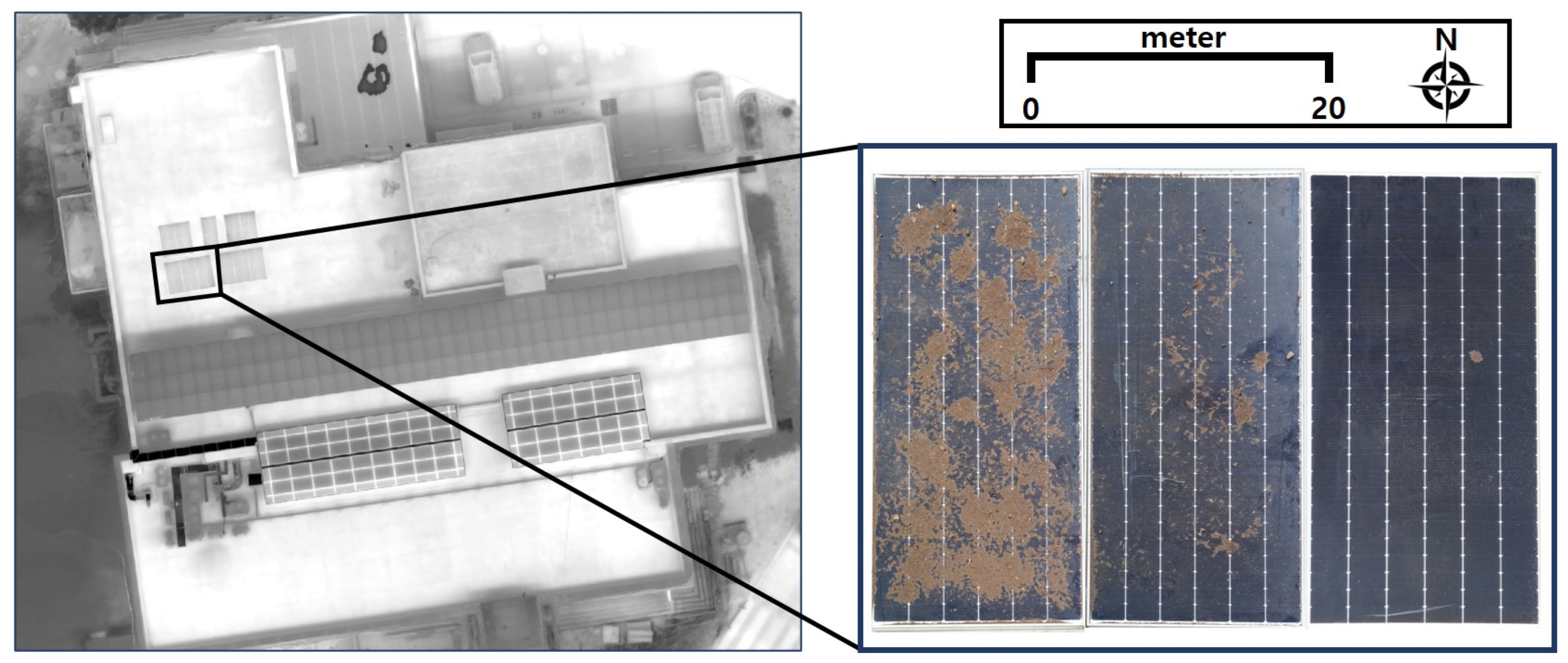
2.1. Study Area

In this study, we set three testbeds of solar modules with a different soil debris-covered area of solar cells in Bokhyeon hall, Kyungpook National University (KNU), Daegu, southeastern South Korea (Figure 1). Testbeds made up of three solar modules are established with different soil debris-covered areas (Testbed 1: 50%; Testbed 2: 5%; Testbed 3: 0.1%) to evaluate the tracking capabilities of autopilot-based and video-based mosaics under the realistic circumstances of the urban area.

KNU is located in the north administrative district in Daegu Metropolitan City, the third most populated city in South Korea. Daegu is called the “Solar City” due to its abundant solar radiation and little precipitation. Therefore, this city is the ideal place for solar power generation. University campuses are well known as the living lab of the urban area since they exhibit spatial variation similar to city-specific landscapes containing a variety of buildings, such as those for vehicle traffic areas, road, green space, libraries, parking lots, lectures, dormitories, and so on [24,25,26]. Furthermore, the city center’s typical land-use patterns and characteristics are shown at the KNU area, such as commercial and business centers, parks, high- and low-rise buildings, dormitories, road networks, playgrounds, green spaces, and other mixed uses [27]. Therefore, it is expected that the solar panels installed in KNU can serve as an ideal testbed for setting allowable errors or parameters for evaluating the tracking capability of solar panel malfunctioning caused by soil debris between the video stream and photo-mosaic at a city-wide scale.

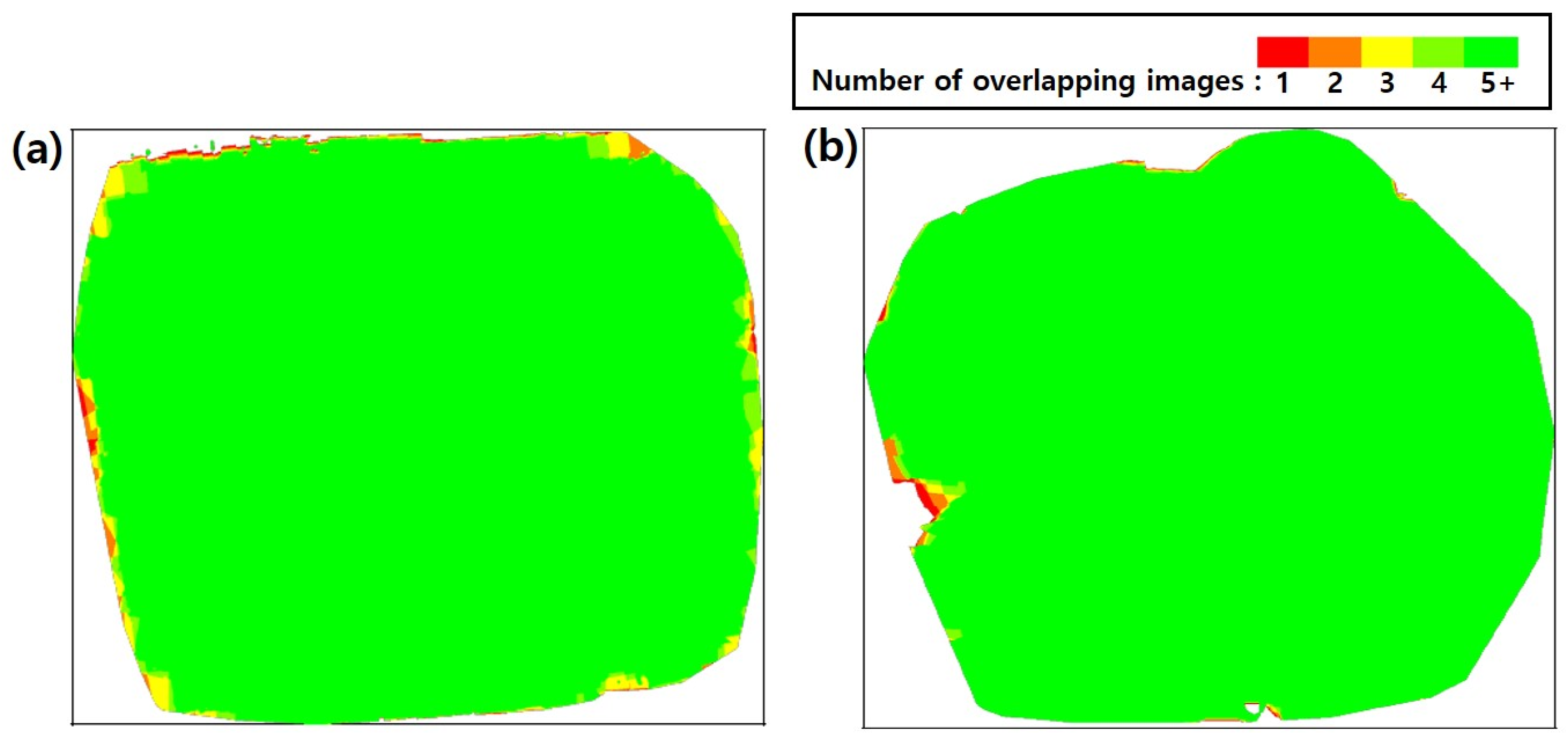
2.2. Data Collection

The UAV video was recorded on 6 August 2021, when the highest solar zenith angle (13:00) to avoid shade and poor weather (for instance, rainfall) occurred. The UAV thermal video was recorded using a quadcopter DJI Matrice 200 V2, equipped with a Zenmuse XT2 camera (

Table 1. Specifications of UAV and thermal camera.

UAV (DJI Matrice 200 V2)			Camera (DJI Zenmuse XT2)
Weight		4.69 kg	Pixel numbers (width × height)	640 × 512
Maximum flight altitude		3000 m (flight altitude used in this experiment: 80 m)	Sensor size (width × height)	10.88 mm × 8.7 mm
			Focal length *	19 mm
			FOV/IFOV	32° × 26°/0.895 mr
Hovering accuracy	z (height)	Vertical, ±0.1 m Horizontal, ±0.3 m	Spectral band	7.5–13.5 μm
			ISO	128
	x, y (location)	Horizontal, ±1.5 m or ±0.3 m (Downward Vision System)	Full frame rates	30 Hz
			Exposure value	4.55
Maximum flight speed		61.2 km/h (P-mode)	Sensitivity [NEDT]/Aperture	<0.05 °C, f/1.0

* Focal length of Zenmuse XT2 is fixed at 19 mm while capturing video and still imageries in autopilot mode. NEDT: Noise equivalent differential temperature.

). The testbeds (Canadian Solar HiDM 400W, CS1U-400MS, 992 × 2078 mm) consist of three solar modules with 162 half solar cells (green dotted line). Shingled solar modules are assembled with an imbricated structure on cells, which are interconnected directly similar to roof tiles. No visible busbars are another characteristic of shingled-type solar modules [28]. Chaichan and Kazem (2020) address that the illumination intensity on the solar cell is reduced according to the amount of deposited soil [29]. As the transmittance radiance is reduced by over 2%, the average solar cell productivity (voltage, current and power) is decreased severely. Reduction in solar cell productivity is relatively stable at the 2–20% reduction of transmittance radiance on the solar cell. Solar cell productivity keeps decreasing as the transmittance reduction is over 20% reduction in transmittance radiance. Thereby, we set the three types of testbeds with the soil debris-covered area differently, distributed based on variations in solar cell productivity: (1) Testbed 1: over 80% of solar module area covered with soil debris; (2) Testbed 2: from 10–20% of solar module area covered with soil debris; (3) Testbed 3: under 1% of solar module area covered with soil debris.

To detect the thermal deficiency of the solar cells in the testbeds, the ground sampling distances (GSD) of thermal still imageries and video frames should be less than 16 cm. Therefore, the GSD of a UAV video can be estimated with the sensor width of the camera ($Sw$), flight height ($H$), focal length of the camera ($F_R$), and image width ($imW$), as follows (Equation (1)):

$$GSD=\frac{Sw\times H\times 100}{F_R\times imW}$$

(1)

Because the camera specifications are fixed, flight height is the main factor to determine the GSD. For this reason, we set the flight altitude to 30 m to attain the best GSD (2.68 cm) available for detecting individual thermal deficiency on solar cells in the study area while leaving sufficient space for the UAV to fly freely over the solar panels. As a result, thermal infrared (TIR) video in the form of a sequence-formatted (SEQ) file was captured at 30 frames per second and flight speed of 2.7 m/s at 30 m flight altitude.

2.3. Thermal Video Frame Mosaic

Raw UAV thermal video itself does not contain geometric information. However, DJI Matrice 200 V2 and Zenmuse XT2 provide telemetry data for full orientation (position and altitude) in subtitle format (SubRip Subtitle: SRT) along with the recorded thermal video. The time sync function of OSDK V3.8.1 embedded in the flight controller of DJI Matrice 200 V2 lines up the observation time of the video, GPS time, and the flight controller clock at 1 Hz. Thus, the SRT file gives second-by-second full orientation data with a number indicating the sequence, Coordinated Universal Time (UTC), and full orientation parameters (GPS coordinates, barometer altitude) acquired from the flight controller during the flight. We utilized Thermal FLIR Studio PRO to extract thermal video frames from the SEQ video file. The full frame rate of DJI Zenmuse XT2 is 30 Hz (30 frames per second). According to Hwang et al. (2021) [23], as the frame intervals are short (15 frames/2 s), the obtained thermal signatures from the video-mosaic are well aligned with the photo-mosaic. Thus, we set the frame intervals for building video-mosaics as 15 frames/2 s with 99% overlapping rates. Autopilot flight is executed over a double-grid path with an overlapping rate of 95%. A mosaic of respective imageries is automatically conducted by utilizing the photogrammetry software Pix4D Mapper following the procedures: (1) Initial processing (key-point extraction, key-point matching, camera model optimization, geolocation GPS/GCP); (2) Point cloud and mesh generation (point densification, 3D textured mesh); and (3) Digital Surface Model (DSM) (photo-mosaic and index) development.

Currently, one of the most widely used methods for geometric correction of UAV imagery is based on Structure-from-Motion (SfM) algorithms. These algorithms provide the opportunity to create accurate 3D models from image structures without prior information about the location at the time of image acquisition or about the camera parameters. With the SfM method, the 3D scene geometry and camera motion are reconstructed from a sequence of 2D images taken by a camera that moves around the scene. The SfM algorithm detects the common 16 feature points in multiple images and uses them to reconstruct the movement of those points throughout the image sequence. With this information, the locations of those points can be calculated and visualized as a 3D point cloud [30]. SfM algorithm is applied to establish the camera exposure position and motion trajectory for building a sparse point cloud [31,32,33,34,35]. The sparse point cloud is then used for camera calibration, and a multiview stereo (MVS) is utilized in conjunction with the DSM generation method based on reverse distance weight interpolation to construct a dense point cloud [36,37]. Figure 2 presents the overlap between the mosaic generated using still imagery (photo-mosaic) and video frames (video-mosaic). Green areas in Figure 2 indicate an overlap of more than five images. The photo-mosaic and video-mosaic are mostly overlapped with more than five images, except borders. The overlap ratios, key-points, and matched key-points are enough to generate high-quality results (Figure 2).

Table 2. Descriptive statistics of detected SCST (°C) in the photo-mosaic and video-mosaic.

Category		Photo-Mosaic	Video-Mosaic
SCSTs of solar cells detected in testbeds (°C)	Min	58.7	60.0
	Max	75.8	76.3
	Mean	68.0	68.6
	Standard deviation	2.00	2.15
Numbers of detected solar cells		8316	8316
Overlapping rates (%)		95	97

presents the surface temperature of solar cells (hereinafter referred to as the SCST) that appeared in the photo-mosaic and video-mosaic.

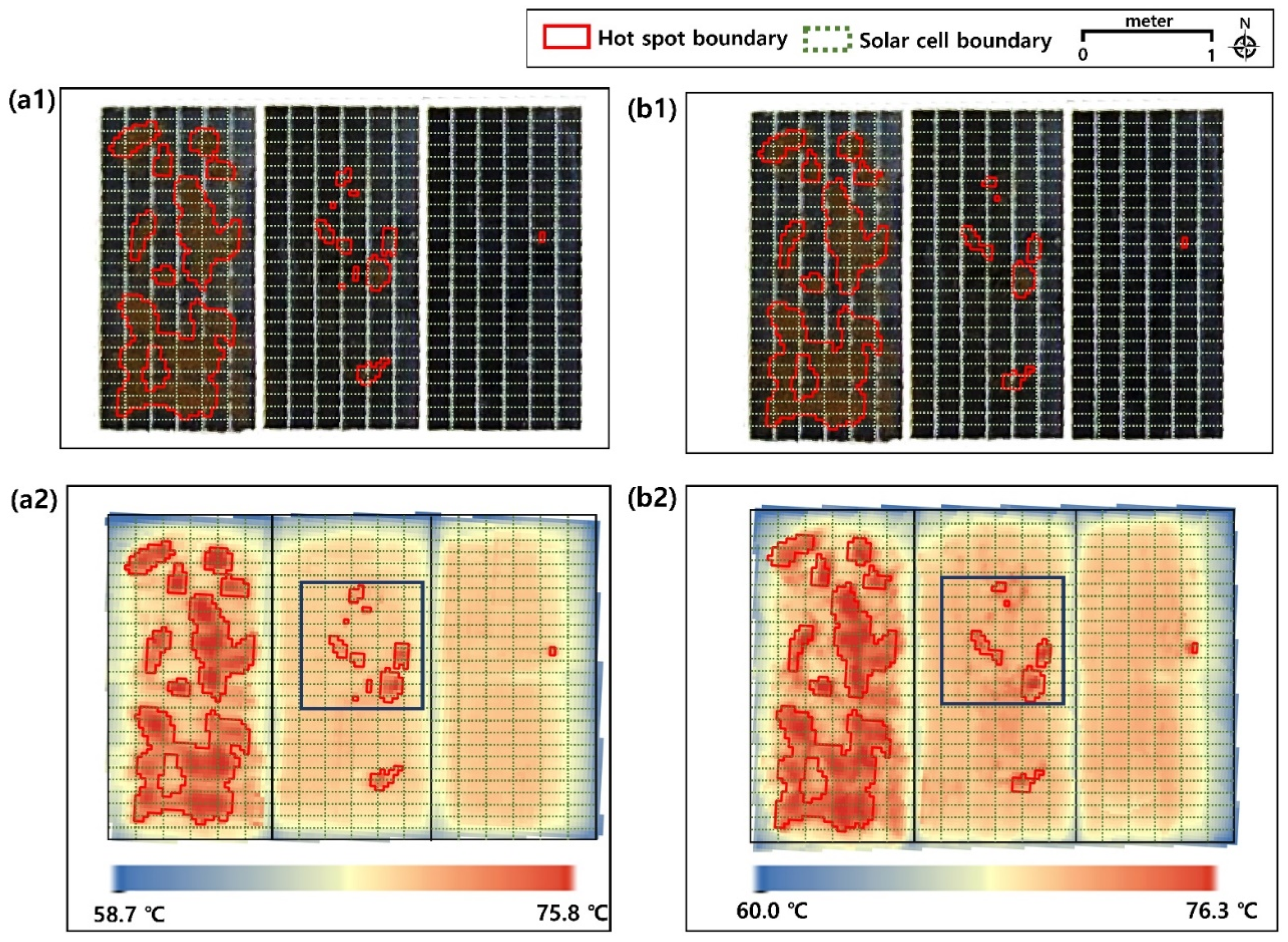
2.4. Hot Spot Analysis (Getis-Ord Gi*)

Spatial autocorrelation is based on the first law of geography in Tobler’s (1970), “everything is related, but the closer is more related than the distant.” Getis-ord Gi* is one of the spatial autocorrelation techniques, which statistically measures the degree of spatial autocorrelation and tests the null hypothesis that the region of interest does not show any spatial pattern other than accidental distribution [38]. We have explored the adjacent distance and pattern of the SCST in solar cell malfunction caused by soil in the photo-mosaic and video-mosaic through hot spot analysis with ArcMap 9.3. After the hot spot analysis, we have evaluated the distribution of the SCSTs at that location to determine whether the spatial patterns of the SCSTs appear the same in the photo-mosaic and video-mosaic. In this study, the Getis-Ord Gi* statistic is calculated through the weight of the space by using the SCSTs. As a result, the spatial clustering can be determined through the high and low values of the calculated p-values and z-scores. The formula for calculating the Getis-Ord Gi* statistic is as follows [39]:

$$G^{*}{}_i=\frac{{{\displaystyle \sum }}_{j=1}^n{w}_{i,j}{x}_j-\overline{X}{{\displaystyle \sum }}_{j=1}^n{w}_{i,j}}{\sqrt{\frac{n{{\displaystyle \sum }}_{j=1}^n{w}_{i,j}{}^2-{({{\displaystyle \sum }}_{j=1}^n{w}_{i,j})}^2}{n-1 }}}$$

(2)

$$\overline{X}=\frac{{{\displaystyle \sum }}_{j=1}^n{x}_j}{n}$$

(3)

$$S=\sqrt{\frac{{{\displaystyle \sum }}_{j=1}^n{x}_j{}^2}{n }}-{(\overline{X})}^2$$

(4)

where $x_j$ is the SCSTs for the $j$ point, $w_{i,j}$ is the spatial weight between the $i$ and $j$ points, and $n$ is the total SCSTs. The Getis-Ord Gi* statistic, calculated by considering the distance between points, determines statistical significance through the $z$-test. In other words, it is determined through statistical significance how much the high and low values of SCSTs are concentrated. If the z-score is positive (+), it is determined that high values are spatially clustered, and if the z-score is a negative (−) value, low values are determined to be spatially clustered.

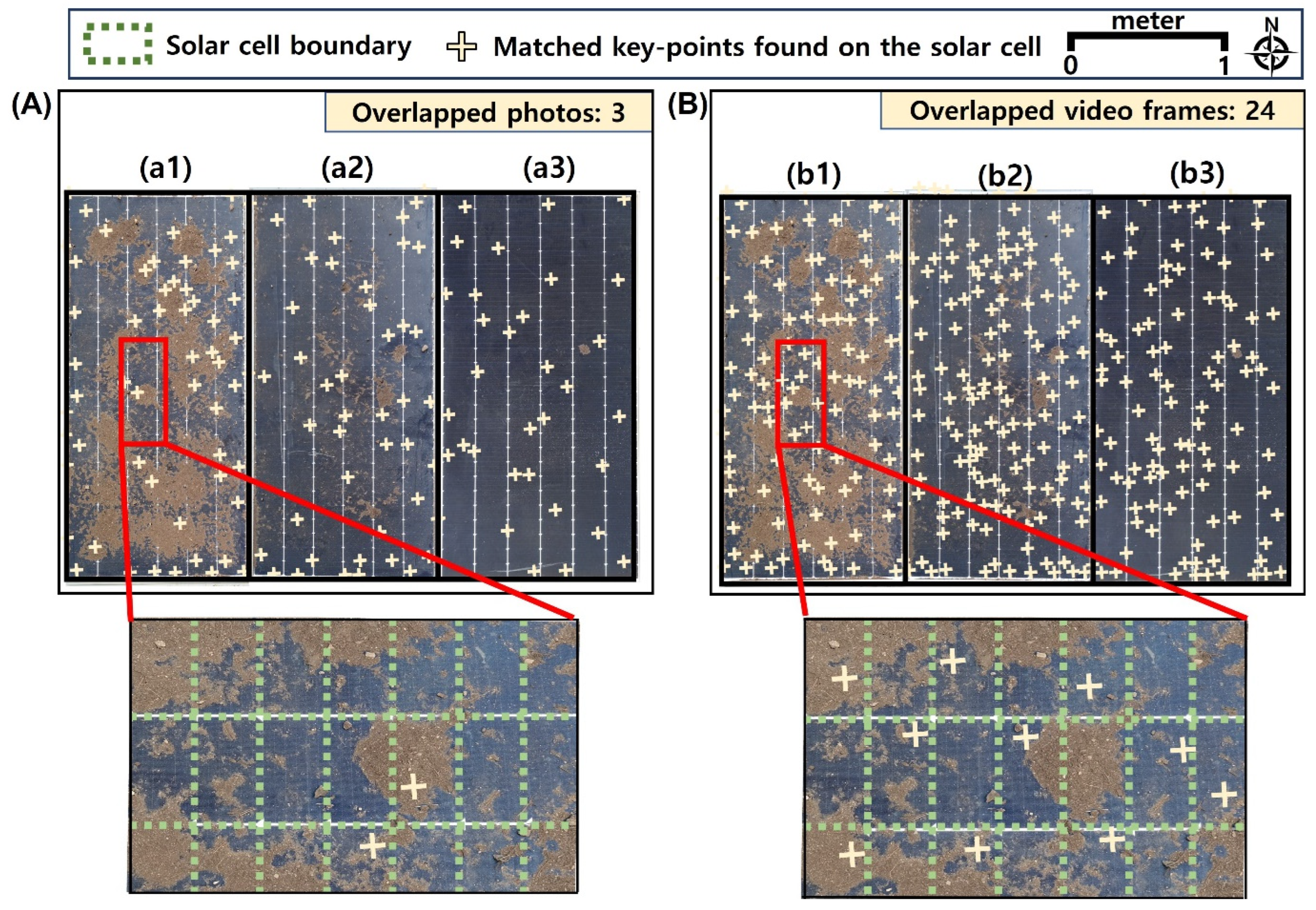
2.5. Evaluating the Performance of Video-Mosaic

2.5.1. Ordinary Least Squares (OLS) Linear Regression

Linear regression assumes stationary relationships across the study area. Linear regression and Pearson correlation analyses explain the linear relationship between the two variables based on proportional equations [40,41,42]. Comparative evaluations with linear regression and Pearson correlation can yield the fitness of the SCSTs of malfunctioning solar cells caused by soil debris detected from the photo-mosaic and video-mosaic. The coefficient and error terms help us determine whether the SCSTs obtained from the video-mosaic are over- or under-measured compared to those of the photo-mosaic in detecting the thermal deficiency on the solar cells. The Pearson correlation indicates that the SCSTs of the video-mosaic and photo-mosaic have the same directions within the malfunctioning points caused by soil debris in the solar cell.

Given that the coefficient and error terms are close to 1 and 0, individually, when the Pearson correlation values are higher, the respective SCSTs gained from the photo-mosaic and video-mosaic are equivalent and have the similar capability in thermal deficiency inspections of solar cell malfunctioning caused by soil debris in terms of thermal signatures. Therefore, the corresponding linear regression models are established with the SCSTs of detected malfunctioning points resulting from soil debris in the video-mosaic (explanatory variables) and photo-mosaic (dependent variables). These linear models, which are expressed as Equations (5) and (6), are calibrated using ordinary least squares (OLS) estimation.

$$SCS{T}_{p1}=a_0+a_1\left(SCS{T}_{\mathrm{v}1}\right)+{\epsilon }_1$$

(5)

$$SCS{T}_{p2}=b_0+b_1\left(SCS{T}_{\mathrm{v}2}\right)+{\epsilon }_2$$

(6)

where $SCS{T}_{p1}$ is the SCSTs of hotspots in Testbed 1 detected from the photo-mosaic, $SCS{T}_{p2}$ is the SCSTs of hotspots in Testbed 2 and Testbed 3 detected from the photo-mosaic, $SCS{T}_{v1}$ is the SCSTs of hotspots in Testbed 1 detected from the video-mosaic, and $SCS{T}_{v2}$ is the SCSTs of hotspots in Testbed 2 and Testbed 3 detected from the video-mosaic. In Equations (5) and (6), $a_1$ and $b_1$ are the coefficients, and ${\epsilon }_1$ and ${\epsilon }_2$ are the random error term of the residuals.

2.5.2. Histogram-Based Correlation

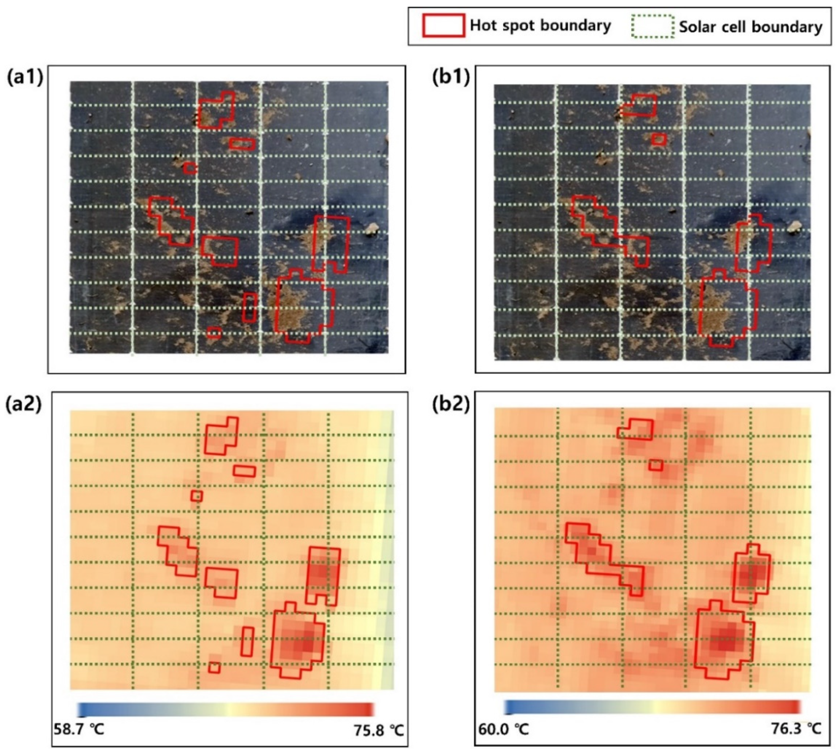
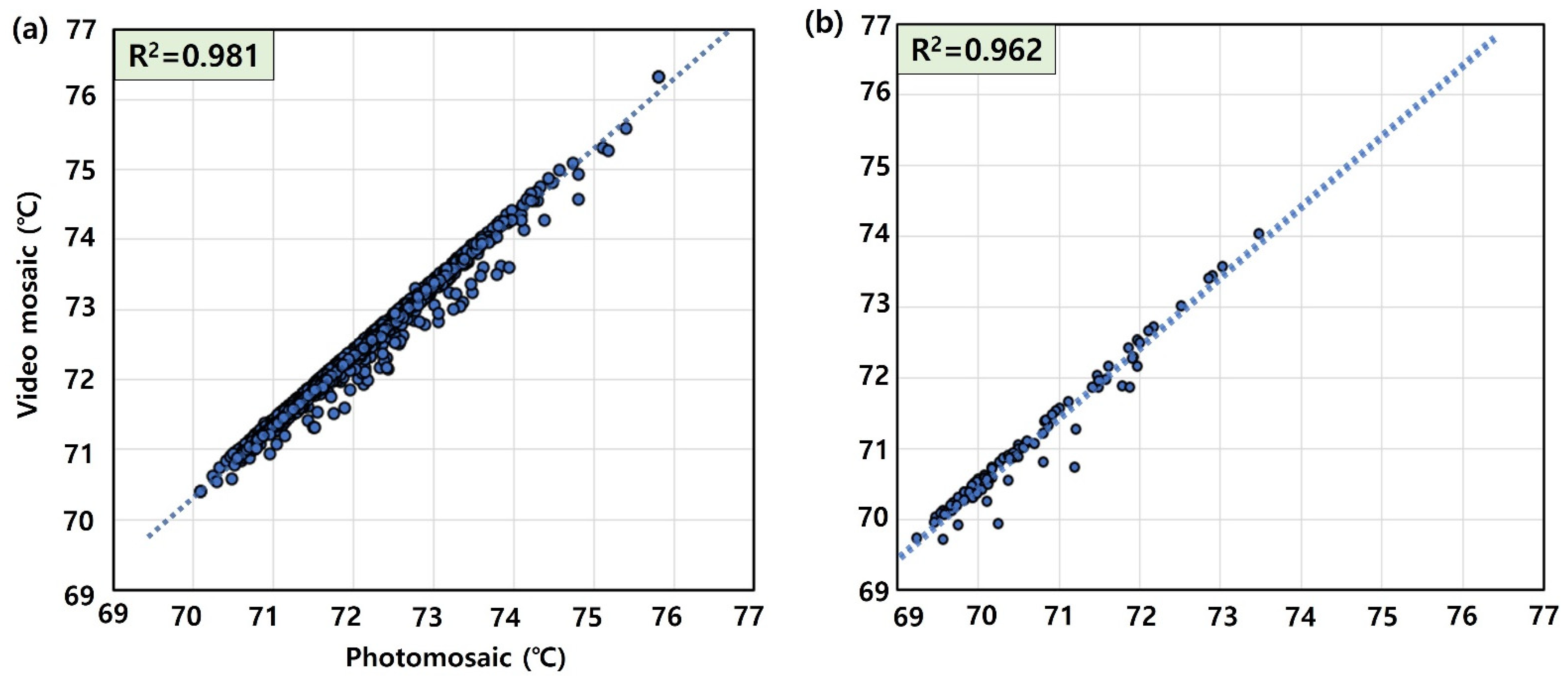
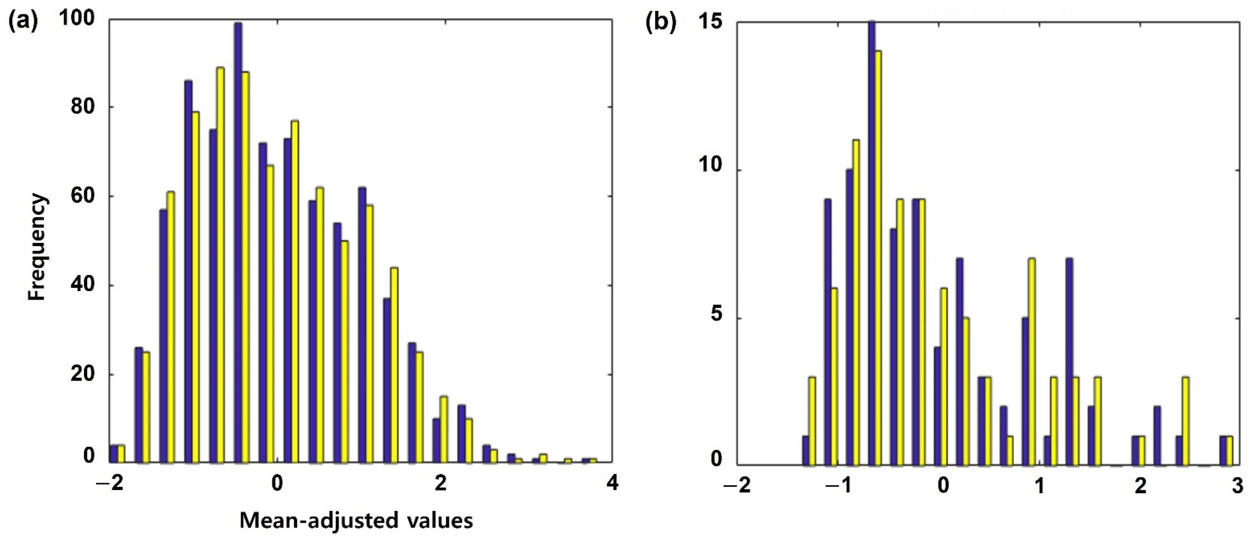
Histogram-based correlation is generally utilized to verify a specific target’s feature extractions or image segmentation by comparing the threshold and distributional similarity between the experimental and control groups [43,44]. For example, the histogram-based correlation can present the differences from extracted features regarding thermal deficiency on solar cells caused by soil debris between the control group (photo-mosaic) and experimental group (video-mosaic) [45,46]. Here, we have conducted a histogram-based correlation to evaluate the distributional properties within hot spots on solar cells caused by soil debris between the control group (photo-mosaic) and experimental group (video-mosaic) with MATLAB R2021a. Note that because the sample is not bivariate, i.e., observations are not measured at the same time instances, we base our measures on the histograms. For example, let us assume $X_i$ and $Y_j$ are distributed according to size to $N$ equidistant bins with resulting relative frequencies $f_n$ and $g_n,n=1,\dots ,N$. Then, the histogram-based correlation is computed as:

$${\rho }_{hist}=\frac{Cov\left(f_n,g_n\right)}{\sqrt{Var\left(f_n\right)Var\left(g_n\right)}}=\frac{{{\displaystyle \sum }}_n\left(f_n-\overline{f}\right)\left(g_n-\overline{g}\right)}{{{\displaystyle \sum }}_n{\left(f_n-\overline{f}\right)}^2{\left(g_n-\overline{g}\right)}^2}$$

(7)

3. Results

A single video frame has a lower resolution than the still photo. However, the video frame has a greater number of key-points per cubic meter (48.5–53.4/m³) in the process of building a mosaic, compared to the still photo (14.1–26.2/m³), as shown in

Table 3. Comparative evaluation of point cloud between the video-mosaic versus the photo-mosaic.

Category	Matched Key-Points per m3			Matched Key-Points per Solar Module
	Testbed 1	Testbed 2	Testbed 3	Testbed 1	Testbed 2	Testbed 3
Photo-mosaic	26.2	21.8	14.1	54	45	29
Video-mosaic	52.4	53.4	48.5	108	110	100

. Furthermore, the video shows far more matched key-points (100–110) than the photos (29–54) per solar module (162 solar cells). Therefore, the video-mosaic has approximately 2.5–3.4 times more matched key-points per solar module than the photo-mosaic (Figure 3). Since autopilot takes pictures over a large area at a higher altitude, only three still photos can be used to generate the mosaic on the investigated solar panel [47]. Contrary, 24 video frames acquired on the solar panel can guarantee more matched key-points due to the constant and consecutive overlap.

Figure 4 and

Table 4. Results of the hot spot analysis (Getis-Ord Gi). The similarity is calculated by dividing hot spots by the matched numbers of hot spots between the photo-mosaic and video-mosaic.

Category		Photo-Mosaic			Video-Mosaic
		Testbed 1	Testbed 2	Testbed 3	Testbed 1	Testbed 2	Testbed 3
Numbers of pixels		809	106	2	767	88	2
z-score of Getis-Ord Gi *	Min	1.962	1.963	2.112	1.961	1.962	2.041
	Max	6.199	5.958	2.218	5.292	5.766	2.046
	Mean	3.139	2.905	2.215	3.027	2.881	2.044
SCSTs in hot spots (°C)	Min	69.6	68.7	70.0	70.4	69.7	70.4
	Max	75.8	73.3	70.4	76.3	74.1	70.9
	Mean	71.8	70.3	70.2	72.4	71.1	70.6
	Standard deviation	1.03	0.95	0.21	0.98	0.97	0.26
The similarity of spatial patterns of hotspots between photo-mosaic vs. video-mosaic (%)		94	81	100	99	97	100

* p-value < 0.05.

contain the results of the hot spot analysis of SCSTs in Testbed 1 to 3 between the photo-mosaic versus the video-mosaic. Mean z-scores are lower in Testbed 3 (soil debris occupying under 1% of a solar module) and higher in Testbed 1 (soil debris occupying over 80% of a solar module) than other testbeds from both the photo-mosaic and video-mosaic. The results of hot spot analysis exhibit that high values of SCST are clustered on malfunctioned solar cells resulting from soil debris in both the photo-mosaic and video-mosaic (Figure 4). The video-mosaic shows similar mean z-scores (2.04–3.03) to the photo-mosaic (2.22–3.14) from Testbed 1 to 3. This implies that the video-mosaic has similar spatial patterns to hot spots derived from the photo-mosaic. The similarity of the spatial patterns of hot spots is over 90% in Testbed 1 and 3 between the photo-mosaic versus the video-mosaic. Testbed 2 (soil debris taking up under 10–20% of a solar module) shows the lowest similarity as 81%. In Figure 5, we present the magnified portion of the photo-mosaic and video-mosaic with hot spot boundary and in situ photos in Testbed 2. Higher values of SCSTs are well presented on most soil-covered solar cells in the video-mosaic. Higher values of SCSTs are more scattered in the video-mosaic than photo-mosaic (Table 4).

4. Discussion

Table 5. Results of the ordinary least squares linear regression with SCSTs (°C) in matched hot spots between the photo-mosaic and video-mosaic.

Frame Intervals	Testbed 1	Testbed 2 & Testbed 3
Numbers of pixels	762	88
Unstandardized coefficient (°C)	1.003 *	0.973 *
t-statistic	199.847 *	46.949 *
VIF	1.000	1.000
Pearson correlation	0.991	0.981
R2	0.981	0.962
RMSE (°C)	0.136	0.183

* p-value < 0.05; VIF: Variance Inflation Factor; RMSE: Root Mean Square Error.

and Figure 6 show the results of the regression analysis to examine the SCSTs detected common hot spots from both the video-mosaic and photo-mosaic in testbeds. $SCS{T}_{\mathrm{v}1}$ and $SCS{T}_{\mathrm{v}2}$ exhibit strong correlations with $SCS{T}_{p1}$ and $SCS{T}_{p2}$ because the Pearson correlation coefficients are higher than 0.98 (0.981–0.991). Moreover, the model fitness values are extremely high at 0.981–0.962. Furthermore, the unstandardized coefficients representing the direction and strength of SCSTs detected from the photo- and video-mosaic is 0.973–1.003, indicating a strongly positive (+) linear correlation. That means that the increases in SCSTs from defective solar cells are likely to point in the same direction. By contrast, the model for Testbeds 2 and 3 has a lower unstandardized coefficient than Testbed 1. Therefore, this indicates that the $SCS{T}_{\mathrm{v}2}$ has higher SCSTS than $SCS{T}_{p2}$ (Figure 6) [49].

Similar results can be found when testing the null hypothesis that the individual models’ coefficients ($a_1,b_1)$ are zero. To validate the null hypothesis, we calculated the t-statistics and p-values. The p-value denotes the highest error probability at which we cannot reject $H_0$: “There is no difference between both distributions” against an alternative $H_A$: “There is a statistically significant difference between both distributions.” Since all p-values are under 0.05, we can reject $H_0$ based on our data. The identical result holds for the t-statistics: $\sqrt{n}*\overline{X}/S,$ where $\overline{X}$ and S are defined as the sample mean and standard deviation. N denotes the sample size. Generally, higher t-statistic values indicate that we can reject $H_0$, that is, that the corresponding coefficients are more likely to be significant. The precise boundary between significance and insignificance depends on the sample size and the Student t-distribution [50]. In Testbeds 2 and 3, the t-statistic values are lower than Testbed 1 (199.847→46.949). The RMSE in Testbeds 2 and 3 is slightly higher than Testbed 1 (0.136 °C→0.183 °C). However, in general, the benchmark of the t-statistic is lower than 3. Hence, the coefficients are statistically significant given the t-statistic values in Table 5.

The distributional similarity of SCSTs in matched hot spots on malfunctioning solar cells caused by soil debris between the photo-mosaic and video-mosaic could present the distributional properties of the recorded observations—both from Testbed 1 and Testbeds 2 and 3. For this purpose, we first must adjust both sets of observations by the mean to account for the temporal recording difference of about 30 min, which is enough to significantly skew the measured temperatures. Let $aut{o}_i$ denote the $i$th temperature observations from a photo-mosaic and $vide{o}_j$ the $j$th temperature observed using video-mosaic. Then, we consider $X_i=aut{o}_i-\overline{aut{o}_i}$ and $Y_j=vide{o}_j-\overline{vide{o}_j}$.

There are different options to compare the distributional properties. Most methods assume that the underlying observations are Gaussian distributed [51]. A quick look at the histograms (Figure 7) and the skewness values (see

Table 6. Descriptive statistics of the histogram with the mean-adjusted SCSTs in matched hot spots between the photo-mosaic and video-mosaic.

Testbed		Min	Max	Mean	Standard Deviation	Skewness	Kurtosis	${\mathit{\rho }}_{\mathit{h}\mathit{i}\mathit{s}\mathit{t}}$ (%)
1	Photo-mosaic	70.1	75.8	72.1	0.99	0.48	2.72	98.95
	Video-mosaic	70.4	76.3	72.5	0.98	0.50	2.74
2 & 3	Photo-mosaic	69.2	73..5	70.6	0.95	0.96	3.18	90.52
	Video-mosaic	69.7	74.0	71.0	0.96	1.04	3.49

) indicate that all distributions are significantly skewed to the right. For $n=20$ the Testbed 1, we find a histogram correlation of ${\rho }_{hist}=98.95\%$; for Testbeds 2 and 3, the value lies slightly lower at ${\rho }_{hist}=90.52\%$. These values vary with the number of bins, but the size stays the same and hence the interpretation: we see very high correlation values close to +1, which indicate that both histograms are highly correlated, i.e., fairly identical.

5. Conclusions

This is arguably the first study exploring the tracking capability of soil debris defects between UAV video and photo-mosaic for a single solar cell to the best of our knowledge. Previous literature has not considered the constraints caused by insufficient key-points and data redundancy in thermal deficiency inspection of solar cells as the minimum survey unit for the solar panel. Due to this reason, most previous studies were implemented with autopilot flight focus on evaluating the tracking ability of UAV in the inspection of area-wide solar farms and plants, as a target much wider than a solar cell unit. This study experimentally validated that the video-mosaic can track the solar cell malfunction caused by soil debris at the level of the photo-mosaic in terms of detecting the spatial patterns and distributional property. Furthermore, this study shows that the video-mosaic has good performance, tracking soil debris defects on the single solar cells with 2.5–3.4 times more matched key-points per solar module than the photo-mosaic. The results of this study can serve as significant evidence for applying video stream to thermal deficiency inspection on single solar cells.

References

1. Hussain, A.; Batra, A.; Pachauri, R. An experimental study on effect of dust on power loss in solar photovoltaic module. Renew. Wind. Water Sol. 2017, 4, 9. [Google Scholar] [CrossRef]
2. Paggi, M.; Corrado, M.; Berardone, I. A global/local approach for the prediction of the electric response of cracked solar cells in photovoltaic modules under the action of mechanical loads. Eng. Fract. Mech. 2016, 168, 40–57. [Google Scholar] [CrossRef]
3. IEA. Review of Failures of Photovoltaic Modules; IEA: Paris, France, 2014. [Google Scholar]
4. Zefri, Y.; ElKettani, A.; Sebari, I.; Ait Lamallam, S. Thermal Infrared and Visual Inspection of Photovoltaic Installations by UAV Photogrammetry—Application Case: Morocco. Drones 2018, 2, 41. [Google Scholar] [CrossRef] [Green Version]
5. Lopez-Garcia, J.; Pozza, A.; Sample, T. Long-term soiling of silicon PV modules in a moderate subtropical climate. Sol. Energy 2016, 130, 174–183. [Google Scholar] [CrossRef]
6. Maghami, M.R.; Hizam, H.; Gomes, C.; Radzi, M.A.; Rezadad, M.I.; Hajighorbani, S. Power loss due to soiling on solar panel: A review. Renew. Sustain. Energy Rev. 2016, 59, 1307–1316. [Google Scholar] [CrossRef] [Green Version]
7. Xu, R.; Ni, K.; Hu, Y.; Si, J.; Wen, H.; Yu, D. Analysis of the optimum tilt angle for a soiled PV panel. Energy Convers. Manag. 2017, 148, 100–109. [Google Scholar] [CrossRef]
8. Anana, W.; Chaouki, F.; Laarabi, B.; Dahlioui, D.; Sebbar, M.A.; Barhdadi, A.; Gilioli, V.; Verdilio, D. Soiling impact on energy generation of high concentration Photovoltaic power plant in Morocco. In Proceedings of the 2016 International Renewable and Sustainable Energy Conference (IRSEC), Marrakesh, Morocco, 14–17 November 2016; pp. 234–238. [Google Scholar]
9. Lee, D.H.; Park, J.H. Developing Inspection Methodology of Solar Energy Plants by Thermal Infrared Sensor on Board Unmanned Aerial Vehicles. Energies 2019, 12, 2928. [Google Scholar] [CrossRef] [Green Version]
10. Zhang, P.; Zhang, L.; Wu, T.; Zhang, H.; Sun, X. Detection and location of fouling on photovoltaic panels using a drone-mounted infrared thermography system. J. Appl. Remote Sens. 2017, 11, 016026. [Google Scholar] [CrossRef]
11. Yao, Y.; Hu, Y. Recognition and location of solar panels based on machine vision. In Proceedings of the 2017 2nd Asia-Pacific Conference on Intelligent Robot Systems (ACIRS), Wuhan, China, 16–18 June 2017; pp. 7–12. [Google Scholar]
12. Jurca, T.; Tulcan-Paulescu, E.; Dughir, C.; Lascu, M.; Gravila, P.; Sabata, A.D.; Luminosu, I.; Sabata, C.D.; Paulescu, M. Global Solar Irradiation Modeling and Measurements in Timisoara. Am. Inst. Phys. 2011, 1387, 253–258. [Google Scholar] [CrossRef]
13. Um, J.-S.; Wright, R. ‘Video Strip Mapping (VSM)’ for Time-sequential Monitoring of Revegetation of a Pipeline Route. Geocarto Int. 1999, 14, 24–35. [Google Scholar] [CrossRef]
14. Um, J.S.; Wright, R. A comparative evaluation of video remote sensing and field survey for revegetation monitoring of a pipeline route. Sci. Total Environ. 1998, 215, 189–207. [Google Scholar] [CrossRef]
15. Um, J.S.; Wright, R. Video strip mosaicking: A two-dimensional approach by convergent image bridging. Int. J. Remote Sens. 1999, 20, 2015–2032. [Google Scholar] [CrossRef]
16. Nguyen, H.V.; Tran, L.H. Application of graph segmentation method in thermal camera object detection. In Proceedings of the 2015 20th International Conference on Methods and Models in Automation and Robotics (MMAR), Miedzyzdroje, Poland, 24–27 August 2015; pp. 829–833. [Google Scholar]
17. Leira, F.S.; Johansen, T.A.; Fossen, T.I. Automatic detection, classification and tracking of objects in the ocean surface from UAVs using a thermal camera. In Proceedings of the 2015 IEEE Aerospace Conference, Big Sky, MT, USA, 7–14 March 2015; pp. 1–10. [Google Scholar]
18. Gómez-Candón, D.; Virlet, N.; Labbé, S.; Jolivot, A.; Regnard, J.-L. Field phenotyping of water stress at tree scale by UAV-sensed imagery: New insights for thermal acquisition and calibration. Precis. Agric. 2016, 17, 786–800. [Google Scholar] [CrossRef]
19. Wu, J.; Dong, Z.; Zhou, G. Geo-registration and mosaic of UAV video for quick-response to forest fire disaster. In Proceedings of the MIPPR 2007: Pattern Recognition and Computer Vision, Wuhan, China, 15–17 November 2007; p. 678810. [Google Scholar]
20. Lafkih, S.; Zaz, Y. Video Solar Plant Monitoring. In Proceedings of the 2017 International Renewable and Sustainable Energy Conference (IRSEC), Tangier, Morocco, 4–7 December 2017; pp. 1–4. [Google Scholar]
21. López-Fernández, L.; Lagüela, S.; Fernández, J.; González-Aguilera, D. Automatic Evaluation of Photovoltaic Power Stations from High-Density RGB-T 3D Point Clouds. Remote Sens. 2017, 9, 631. [Google Scholar] [CrossRef] [Green Version]
22. Hwang, Y.-S.; Schlüter, S.; Park, S.-I.; Um, J.-S. Comparative Evaluation of Mapping Accuracy between UAV Video versus Photo Mosaic for the Scattered Urban Photovoltaic Panel. Remote Sens. 2021, 13, 2745. [Google Scholar] [CrossRef]
23. Hwang, Y.-S.; Schlüter, S.; Lee, J.-J.; Um, J.-S. Evaluating the Correlation between Thermal Signatures of UAV Video Stream versus Photomosaic for Urban Rooftop Solar Panels. Remote Sens. 2021, 13, 4770. [Google Scholar] [CrossRef]
24. Robertson, S. Campus, City, Networks and Nation: Student-Migrant Activism as Socio-spatial Experience in Melbourne, Australia. Int. J. Urban Reg. Res. 2013, 37, 972–988. [Google Scholar] [CrossRef]
25. Srivanit, M.; Hokao, K. Evaluating the cooling effects of greening for improving the outdoor thermal environment at an institutional campus in the summer. Build. Environ. 2013, 66, 158–172. [Google Scholar] [CrossRef]
26. Hwang, Y.-S.; Um, J.-S. Comparative Evaluation of Cool Surface Ratio in University Campus: A Case Study of KNU and UC Davis. KIEAE J. 2015, 15, 117–127. [Google Scholar] [CrossRef] [Green Version]
27. Park, S.-I.; Um, J.-S. Differentiating carbon sinks versus sources on a university campus using synergistic UAV NIR and visible signatures. Environ. Monit. Assess. 2018, 190, 652. [Google Scholar] [CrossRef] [PubMed]
28. Klasen, N.; Mondon, A.; Kraft, A.; Eitner, U. Shingled cell interconnection: A new generation of bifacial PV-modules. In Proceedings of the 7th Workshop on Metallization and Interconnection for Crystalline Silicon Solar Cells, Konstanz, Germany, 23–24 October 2017. [Google Scholar]
29. Chaichan, M.T.; Kazem, H.A. Experimental evaluation of dust composition impact on photovoltaic performance in Iraq. Energy Sources Part A Recovery Util. Environ. Eff. 2020, 1–22. [Google Scholar] [CrossRef]
30. Verhoeven, G. Taking computer vision aloft—Archaeological three-dimensional reconstructions from aerial photographs with photoscan. Archaeol. Prospect. 2011, 18, 67–73. [Google Scholar] [CrossRef]
31. Lee, J.-J.; Hwang, Y.-S.; Park, S.-I.; Um, J.-S. Comparative Evaluation of UAV NIR Imagery versus in-situ Point Photo in Surveying Urban Tributary Vegetation. J. Environ. Impact Assess. 2018, 27, 475–488. [Google Scholar] [CrossRef]
32. Um, J.-S. Valuing current drone CPS in terms of bi-directional bridging intensity: Embracing the future of spatial information. Spat. Inf. Res. 2017, 25, 585–591. [Google Scholar] [CrossRef]
33. Park, S.-I.; Hwang, Y.-S.; Lee, J.-J.; Um, J.-S. Evaluating Operational Potential of UAV Transect Mapping for Wetland Vegetation Survey. J. Coast. Res. 2021, 114, 474–478. [Google Scholar] [CrossRef]
34. Um, J.-S. Evaluating patent tendency for UAV related to spatial information in South Korea. Spat. Inf. Res. 2018, 26, 143–150. [Google Scholar] [CrossRef]
35. Um, J.-S. Embracing cyber-physical system as cross-platform to enhance fusion-application value of spatial information. Spat. Inf. Res. 2017, 25, 439–447. [Google Scholar] [CrossRef]
36. Liu, Y.; Zheng, X.; Ai, G.; Zhang, Y.; Zuo, Y. Generating a High-Precision True Digital Orthophoto Map Based on UAV Images. ISPRS Int. J. Geo-Inf. 2018, 7, 333. [Google Scholar] [CrossRef] [Green Version]
37. Park, S.-I.; Hwang, Y.-S.; Um, J.-S. Estimating blue carbon accumulated in a halophyte community using UAV imagery: A case study of the southern coastal wetlands in South Korea. J. Coast. Conserv. 2021, 25, 38. [Google Scholar] [CrossRef]
38. Khan, G.; Qin, X.; Noyce, D.A. Spatial Analysis of Weather Crash Patterns. J. Transp. Eng. 2008, 134, 191–202. [Google Scholar] [CrossRef]
39. Getis, A.; Ord, K. The Analysis of Spatial Association by Use of Distance Statistics. Geogr. Anal. 1992, 24, 189–206. [Google Scholar] [CrossRef]
40. Hwang, Y.; Um, J.-S.; Hwang, J.; Schlüter, S. Evaluating the Causal Relations between the Kaya Identity Index and ODIAC-Based Fossil Fuel CO2 Flux. Energies 2020, 13, 6009. [Google Scholar] [CrossRef]
41. Hwang, Y.; Um, J.-S. Performance evaluation of OCO-2 XCO2 signatures in exploring casual relationship between CO2 emission and land cover. Spat. Inf. Res. 2016, 24, 451–461. [Google Scholar] [CrossRef]
42. Hwang, Y.; Um, J.-S. Evaluating co-relationship between OCO-2 XCO2 and in situ CO2 measured with portable equipment in Seoul. Spat. Inf. Res. 2016, 24, 565–575. [Google Scholar] [CrossRef]
43. Hao, D.; Li, Q.; Li, C. Histogram-based image segmentation using variational mode decomposition and correlation coefficients. Signal Image Video Process. 2017, 11, 1411–1418. [Google Scholar] [CrossRef]
44. Abdollahnejad, A.; Panagiotidis, D.; Surový, P. Estimation and Extrapolation of Tree Parameters Using Spectral Correlation between UAV and Pléiades Data. Forests 2018, 9, 85. [Google Scholar] [CrossRef] [Green Version]
45. Liao, K.-C.; Lu, J.-H. Using UAV to Detect Solar Module Fault Conditions of a Solar Power Farm with IR and Visual Image Analysis. Appl. Sci. 2021, 11, 1835. [Google Scholar] [CrossRef]
46. Bian, J.; Zhang, Z.; Chen, J.; Chen, H.; Cui, C.; Li, X.; Chen, S.; Fu, Q. Simplified Evaluation of Cotton Water Stress Using High Resolution Unmanned Aerial Vehicle Thermal Imagery. Remote Sens. 2019, 11, 267. [Google Scholar] [CrossRef] [Green Version]
47. Um, J.-S. Drones as Cyber-Physical Systems; Springer: Berlin/Heidelberg, Germany, 2019. [Google Scholar]
48. Gadag, R.V.; Shetty, A.N. Engineering Chemistry, 3rd ed.; IK International Pvt Ltd.: New Delhi, India, 2014. [Google Scholar]
49. Hwang, Y.; Um, J.-S.; Schlüter, S. Evaluating the Mutual Relationship between IPAT/Kaya Identity Index and ODIAC-Based GOSAT Fossil-Fuel CO2 Flux: Potential and Constraints in Utilizing Decomposed Variables. Int. J. Environ. Res. Public Health 2020, 17, 5976. [Google Scholar] [CrossRef] [PubMed]
50. Troy, A.; Morgan Grove, J.; O’Neil-Dunne, J. The relationship between tree canopy and crime rates across an urban–rural gradient in the greater Baltimore region. Landsc. Urban Plan. 2012, 106, 262–270. [Google Scholar] [CrossRef]
51. Mudholkar, G.S.; Natarajan, R. The inverse Gaussian models: Analogues of symmetry, skewness and kurtosis. Ann. Inst. Stat. Math. 2002, 54, 138–154. [Google Scholar] [CrossRef]
Figure 1. Mosaic of thermal imageries and an in situ photo of the study site. Black box is the location of experimental targets. The magnified picture (left side) is the in-situ photo of experimental targets.
Remotesensing 14 01220 g001
Figure 2. The number of overlapping images in the thermal mosaic of the experimental site with the point cloud. The green areas indicate a degree of overlap by more than five images. The red and yellow areas indicate a low overlap, resulting in poor mosaic quality. (a) Photo-mosaic; (b) Video-mosaic.
Remotesensing 14 01220 g002
Figure 3. Differentiated distribution density of matched key-points between solar cells of the photo-mosaic and video-mosaic. (A) photo-mosaic; (B) video-mosaic; (a1,b1) Testbed 1; (a2,b2) Testbed 2; (a3,b3) Testbed 3. Solar panel includes one or more solar modules assembled as a pre-wired, field-installable unit [48]. The typical solar module is the aggregation of solar cells, 60 (6 by 10) or 72 (6 by 12) [1]. The magnified picture (red box) of the photo-mosaic (bottom-left) contains only two matched key-points, while the video (bottom-right) shows ten.
Remotesensing 14 01220 g003
Figure 4. Hot spot boundary on solar cells malfunctioning due to soil debris. (a1) Hot spot boundary (derived from photo-mosaic) overlaid on-field photo; (b1) Hot spot boundary (derived from video-mosaic) overlaid on-field photo; (a2) Hot spot boundary detected from photo-mosaic; (b2) Hot spot boundary detected from video-mosaic. The quadrangle (black box) represents the magnified portion presented in Figure 5.
Remotesensing 14 01220 g004
Figure 5. Comparison of magnified image and hot spots between the photo-mosaic and video-mosaic. (a1) in situ photo and hot spot boundary detected from photo-mosaic; (a2) photo-mosaic and hot spot boundary detected from photo-mosaic; (b1) in situ photo and hot spots detected from video-mosaic; (b2) video-mosaic and hot spot boundary detected from video-mosaic. See the location of the image in Figure 4.
Remotesensing 14 01220 g005
Figure 6. Scatter plots of SCSTs in matched hot spots between the photo-mosaic and video-mosaic. (a) Testbed 1; (b) Testbeds 2 and 3.
Remotesensing 14 01220 g006
Figure 7. Absolute frequencies. The blue bar is the mean adjusted values of SCSTs of the video photo-mosaic in matched hot spots. The yellow bar is the mean adjusted values of SCSTs of the photo-mosaic in matched hot spots. (a) Testbed 1; (b) Testbeds 2 and 3.
Remotesensing 14 01220 g007