Abstract
Malagasy subsistence farmers, who comprise 70% of the nearly 26 million people in Madagascar, often face food insecurity because of unreliable food production systems and adverse crop conditions. The 2020–2021 drought in Madagascar, in particular, is associated with an exceptional food crisis, yet we are unaware of peer-reviewed studies that quantitatively link variations in weather and climate to agricultural outcomes for staple crops in Madagascar. In this study, we use historical data to empirically assess the relationship between soil moisture and food production. Specifically, we focus on major staple crops that form the foundation of Malagasy food systems and nutrition, including rice, which accounts for 46% of the average Malagasy caloric intake, as well as cassava, maize, and sweet potato. Available data associated with survey-based crop statistics constrain our analysis to 2010–2017 across four clusters of Malagasy districts. Strong correlations are observed between remotely sensed soil moisture and rice production, ranging between 0.67 to 0.95 depending on the cluster and choice of crop calendar. Predictions are shown to be statistically significant at the 90% confidence level using bootstrapping techniques, as well as through an out-of-sample prediction framework. Soil moisture also shows skill in predicting cassava, maize, and sweet potato production, but only when the months most vulnerable to water stress are isolated. Additional analyses using more survey data, as well as potentially more-refined crop maps and calendars, will be useful for validating and improving soil-moisture-based predictions of yield.
1. Introduction
Madagascar has one of the highest rates of poverty in Africa, with 42% of the country’s children under five experiencing chronic malnutrition and stunting [1]. Farmers comprise approximately 70% of the population and the majority of these farmers are smallholders cultivating for subsistence [2]. Malagasy farmers, particularly smallholders, are extremely vulnerable to disruptions in production due to their high dependence on agriculture for livelihoods, low rate of imports, chronic food insecurity, poor infrastructure, and lack of social safety nets [3,4,5]. For example, the 2020–2021 drought in Madagascar, which is one of the most severe in 30 years [6,7,8], has “created a nutritional crisis of exceptional gravity” according to aid organizations [9].
Understanding how variations in weather affect agricultural production is useful when developing climate adaptation strategies, such as the selection of crops and varieties as well as management of water resources [2,3]. Empirical studies underscore that increasing agricultural production in Madagascar is an important strategy to reduce poverty and food insecurity rates in rural regions [10], where most of the population resides (61% in 2020) [11]. To our knowledge, however, there are no peer-reviewed studies quantitatively linking variations in weather to agricultural outcomes at the sub-national scale across Madagascar. A review of local and regional crop forecasting approaches found no studies focusing on regions within Madagascar, out of 362 studies across 71 other nations [12]. Furthermore, a recent literature review on climate change in Madagascar and set of interviews with Malagasy development agencies, non-government organizations, and other stakeholders identifies information regarding how local climate variations affect agricultural yields as an important information gap [13].
The under-representation of developing nations, like Madagascar, in the crop forecasting literature is variously attributable to the small plot sizes, mixed cropping, limited availability of climate data, and scarcity of crop statistics [12]. For example, empirical crop models that rely on remotely sensed land surface characteristics, which are independent of geopolitical boundaries, still require crop statistics for training, as well as crop distribution maps and crop calendars to isolate the relevant signal from remotely sensed observations [14,15]. Isolating the crop signal from remotely sensed observations can be particularly challenging for measurements with a low spatial resolution [16], but they are nonetheless necessary to use due to their higher return frequency or longer record availability.
In this study, we assess the potential to predict variations in the production of rice, cassava, maize, and sweet potato in Madagascar from 2010 to 2017 using remotely-sensed soil moisture and survey-based crop statistics. These four staple crops account for approximately 75% of daily caloric intake in Madagascar (46.4% for rice, 20.7% for cassava, 5.1% for maize, and 2.4% for sweet potato) [17]. Rice, often eaten at every meal [18], is of key importance to Malagasy people both culturally and nutritionally [3,19,20]. We focus on empirically relating the production of these crops to water availability, as indicated by soil moisture. Such an approach is informed by the fact that droughts are a leading cause of food scarcity in Madagascar [3], especially in the arid south, and that a strong relationship generally exists between water availability and both dry and flooded rice production [21]. Furthermore, the 2010 to 2017 time period encompasses a period of increasing dryness across Madagascar [22]. Soil moisture observations have also been shown to track crop outcomes better than other metrics of water availability, such as precipitation [23,24].
Our primary research objective is to quantify the empirical relationship between soil moisture and the production of rice, cassava, maize, and sweet potato production across Madagascar. Two supporting objectives stem from the facts that location and seasonality of crop growth is critical for assessing relationships with soil moisture. We, therefore, also evaluate the sensitivity of the production-soil moisture relationship to a set of crop distribution maps and crop calendars. Furthermore, because the applicability of existing crop calendars are unclear for the crops we evaluate in Madagascar, we develop and apply a crop calendar based upon the normalized difference vegetation index (NDVI). Throughout this study, we use crop distribution maps, crop calendars, and remotely sensed observations of vegetation and soil moisture that are globally-resolved to facilitate future analogous studies in other developing nations, which are also generally under-represented in the literature [12] and vulnerable to agricultural climate shocks [25], including climate change [26].
2. Materials and Methods
2.1. Study Region
Madagascar encompasses diverse hydroclimates [27]. Trade winds lead to zones of high orographic precipitation along the East; cyclones develop seasonally in the North; and anticyclonic fronts intermittently bring rainfall in the South and West. Annual climatological precipitation in the Southwest is only 350 mm, whereas the East Coast receives 4000 mm [22]. There are generally two distinct seasons: a wet and hot season from November to April and a cool and dry season from May to October. Interannual rainfall, influenced by dynamics associated with the Intertropical Convergence Zone and linkages with the El-Niño Southern Oscillation and Southern Oscillation, is highly variable [22,28,29].
2.2. Data
2.2.1. Satellite-Based Vegetation Activity and Soil Moisture
Remotely sensed vegetation activity is represented by the Normalized Difference Vegetation Index (NDVI) from the MODIS/Terra Vegetation Indices Monthly L3 Global (MOD13C2v006) dataset [30], which is at a 0.05-degree spatial resolution and available from 2000 to present (Figure 1b). This dataset was chosen because it spans the period of interest (2010–2017), provides monthly estimates, and is known to track crop characteristics, as described in recent review articles [14,15]. NDVI from MODIS, for example, has been used to estimate yields (e.g., [31]), identify irrigated regions (as described in the review by [32]), and determine crop phenology (e.g., [33]).
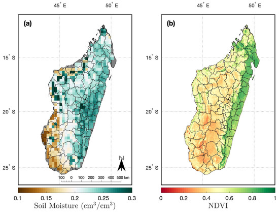
Figure 1.
Satellite-based annual average (a) soil moisture and (b) vegetation activity (NDVI) from 2010 to 2017. Districts are outlined on each map.
Near-surface daily soil moisture observations (in units cm/cm) are from the European Space Agency’s Climate Change Initiative (ESA-CCI) soil moisture project version 5.2 [34,35,36] and are provided at a 0.25-degree spatial resolution (Figure 1a). This data product combines single-sensor active and passive microwave remotely-sensed soil moisture observations from various platforms. Daily soil moisture observations are available from 1979 to the present, with the number of observations increasing over time as new satellites observations become available. This dataset covers the entire period of record from 2010 to 2017, although it should be noted that measurements are only of near-surface soil moisture, down to approximately 5 cm, which is less than the typical crop rooting depth. Soil moisture observations are averaged to the monthly time scale analogous to NDVI and down-scaled to match the 0.05-degree spatial resolution of NDVI using nearest-neighbor interpolation. This down-scaling procedure is used to facilitate spatially weighting soil moisture observations that are, ultimately, averaged to the district-level, whereby each 0.05-degree grid box center that falls within a district boundary is included in the district average, rather than using the native 0.25-degree grid box centers.
2.2.2. Survey-Based Crop Production
We obtain reports of crop production for rice, cassava, maize, and potato from the Malagasy Ministry of Agriculture (Figure 2a–d). Reports of “potato” are interpreted to represent sweet potato, as they align well with the national-level production of sweet potato reported by the Food and Agriculture Organization’s (FAO) Statistics Division (FAOSTAT) (Figure S1). Production is reported for each of the 114 districts, which range in size from 31 km (Toamasina I) to over 17,000 km (Ihosy). To estimate district-level production, the Ministry executed a nationally representative agricultural census in 2004–2005. Fokontany, equivalent to a village, were sampled with equal probability and without replacement at a rate of 30%, with 4407 Fokontany sampled out of a total of 14,299. Randomly-sampled agricultural plots were surveyed for each selected Fokontany such that approximately 7% of all 731,629 farm plots in Madagascar were surveyed. Following 2005, production estimates involved a combination of less-intensive data collection and statistical modeling leveraging the detailed 2004–2005 census. We focus our analysis on explaining crop production, measured in tonnes, rather than crop yield, in tonnes/hectare, because harvested area is unavailable at the district level.
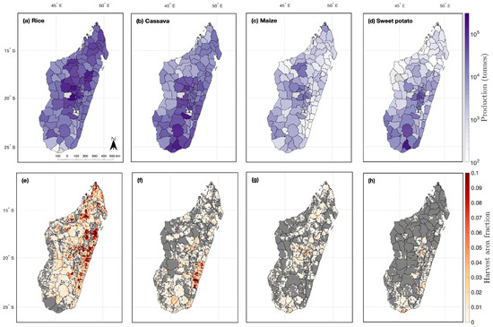
Figure 2.
Survey-based average crop production (in tonnes) for each district, including (a) rice, (b) cassava, (c) maize, and (d) sweet potato and the associated harvested area fractions for (e) rice, (f) cassava, (g) maize, and (h) sweet potato. The harvested area fraction represents the average fractional proportion of a 0.05-degree grid box that was harvested in a crop during the 1997–2003 era [37]. In (e–h), grid boxes with harvested area fractions less than 0.001 are colored gray.
Although district-level production data is nominally available from 2005 to 2017, we analyze the observations only between 2010 to 2017 on account of seemingly anomalous behavior in the data prior to 2010 in two respects. First, cassava and sweet potato production is reported as nearly constant prior to 2010, with an interannual standard deviation of 2.8 × 10 tonnes for cassava prior to 2010, for example, as compared to 3.9 × 10 tonnes from 2010 onward (Figure S1). Second, there are larger disagreements between the sum of the district-level data and national-level statistics provided by FAOSTAT from 2005 to 2009 for all four crops, especially for maize, cassava, and sweet potatoes (Figure S2). For example, average annual absolute differences over time in production for maize, cassava, and sweet potatoes between the two datasets are, respectively, 16,600 tonnes, 41,400 tonnes, and 90,100 tonnes from 2005 to 2009 but only 7000 tonnes, 300 tonnes, and 22,000 tonnes from 2010 to 2017. Note that the median absolute difference between datasets from 2010 to 2017 is less than 2 tonnes for rice, cassava, and maize, reflecting that discrepancies are largely confined to specific years, whereas discrepancies exceed 10 tonnes for each crop for each year between 2005 and 2009.
We focus on production reporting practices, as opposed to physical or observational shifts because there appears no analogous shift in remotely sensed observations of soil moisture and NDVI over the 2005 to 2017 period. In particular, regional anomalies in soil moisture and NDVI remain highly correlated from 2005 to 2017 (Figure S3). These seeming data inhomogeneities are not, however, documented in national-level quality flags from FAOSTAT and district-level data are not associated with quality flags. The lack of documentation and the shortness of the available record leads to our viewing these results as provisional pending further historical or near-present analysis.
2.2.3. Crop Distribution
We select agricultural regions from the gridded remotely-sensed observations using maps of harvested area for rice, cassava, maize, and sweet potato (Figure 2e–h) [37]. These crop-specific harvested area maps are each re-gridded from a 5-minute spatial resolution to the 0.05-degree spatial resolution grid associated with NDVI by finding the nearest observation. Each 0.05-degree grid box is associated with a fractional harvested area of rice, cassava, maize, and sweet potato.
There are other remotely-sensed data products that specify the location of croplands without distinguishing between different crops, such as the MODIS Terra+Aqua Combined Land Cover product (MCD12C1v006) [38] (Figure S4a) and Global Food Security-Support Analysis Data at 30 m (GFSAD30) [39] (Figure S4b). We base our primary results on the crop-specific maps [37] because of large regional differences in where rice, cassava, maize, and sweet potato are grown across Madagascar. One issue in using the crop-specific maps is that they are static and representative of the year 2000, whereas the MCD12C1v006 data are dynamic, changing each year to represent changes in land cover. Interannual variations between 2010 to 2017 in the MCD12C1v006 generic cropland maps are, however, small relative to regional variations between different crops in the crop-specific maps. For example, if we compare spatial variations between crops, we find that 19% of the 0.05-degree grid boxes across Madagascar have a crop factional area greater than 0.001 for sweet potato, while 71% of grid boxes have a crop factional area greater than 0.001 for rice. Temporal variations from the MCD12C1v006 cropland map, on the other hand, indicate that total cropland fractions greater than 0.001 have changed by less than 2% from 2010 to 2017. It follows that the use of crop-specific maps leads to greater skill in predicting production relative to the dynamic MCD12C1v006 map. Results using the generic GFSAD30 and MCD12C1v006 maps are shown in Table S3 and Table S4, respectively.
2.2.4. Crop Calendars
We consider four different calendars for the months in which water availability influences production for each considered crop (Figure 3 for rice; Figures S5–S7 for cassava, maize, and sweet potato). The first two calendars are based on crop-specific growing seasons, starting at a mean planting date and ending at a mean harvesting data. Calendar 1 (Figure 3a,e), referred to as C1, is globally-resolved and frequently used for analyses of crop-climate interactions in other countries and at the global scale [40]. For example, it was used as the main crop calendar in the recent Global Gridded Crop Model Intercomparison (GGCMI) Phase 2 experiment by the Agricultural Model Intercomparison and Improvement Project (AgMIP) [41]. The planting and harvest dates are prescribed as uniform across Madagascar for each of rice, maize, and sweet potato, which is a major simplification given spatial heterogeneity in climate (Figure 1) and planting practices, as indicated by the FAO (described below as Calendar 2). There are some regional variations for cassava in C1, with the center of Madagascar differing from the rest of the country (Figure S5a,e).
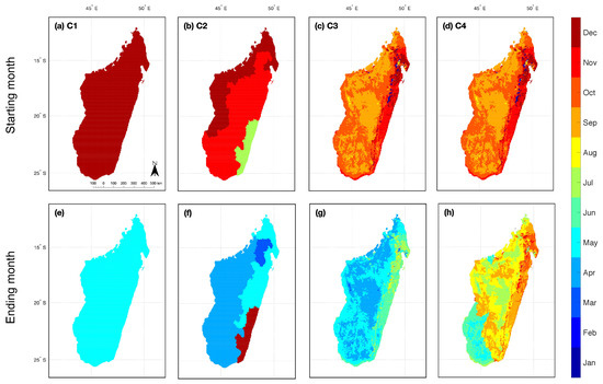
Figure 3.
The four calendars used to temporally average soil moisture anomalies for comparison with rice production anomalies (see Figures S5–S7 for analogous plots of cassava, maize, and sweet potato). The top row represents the starting month of the temporal average for calendars (a) C1, (b) C2, (c) C3, and (d) C4. The bottom represents the ending month of the temporal average for calendars (e) C1, (f) C2, (g) C3, and (h) C4. C1 and C2 represent mean planting (start) and mean harvesting (end) dates, while C3 and C4 represent temporal periods based on NDVI. For C2 (b,f), we have mapped the rainy season calendar (see Figure S8 for separate maps of the rainy and dry seasons and Supplementary Data 1 for details on C2). The starting month for C3 (c) and C4 (d) are identical, as they represent the minimum in NDVI after the climatological seasonal cycle is smoothed with a 5-month moving window. For all calendars, the starting month can be in the year prior to harvest.
The second calendar (C2; Figure 3b,f) comes from the FAO’s Crop Calendar Information Tool (accessed on 16 August 2021, https://cropcalendar.apps.fao.org/). This dataset specifies ranges of crop planting and harvesting dates at the district-level, which we use to estimate the mean planting and harvesting months for each crop and district. C2 contains more spatial heterogeneity than C1 for all four crops. C2 also specifies two rice growing seasons for each district– a rainy growing season and a dry growing season (Figure S8). There are also 35 districts that have a third growing season for rice called the “mid-season”, which falls between the rainy and dry seasons. We merge all three growing seasons (rainy, mid, and dry) for purposes of making evaluations. There is less skill in predicting rice production when the rainy or dry seasons are evaluated separately relative to the merged growing season (Table S5), which follows the fact that reported rice production represents the sum across all seasons. For maize, there is only one growing season specified for each district, while there are occasionally two growing seasons specified for cassava and sweet potato, which we merge for purposes of evaluation similar to rice. We do not assess the mid-season rice or individual growing seasons for cassava or sweet potato separately, as done for dry and rainy season rice (Table S5), because these growing seasons are limited to only small regions of Madagascar. C2 does not specify any growing season for cassava, maize, and sweet potato in certain districts even though the survey data indicates production, in which case we assign growing seasons at the grid-box scale based on the nearest grid box with a specified growing season (Figure S9). The rainy, mid, dry, and merged growing seasons for each crop and district specified by C2 are detailed in Supplementary Data 1.
In Calendars 3 and 4 (C3 and C4), we define a spatially-varying calendar using NDVI [30] that allows for spatial heterogeneity within districts. In particular, our NDVI-based calendar starts in the month of minimum NDVI at a given grid box after smoothing NDVI using a five month running weighted average. We assume the minimum in NDVI signifies the start of a new crop season. In one version (C3; Figure 3c,g), we average across eight months from the starting calendar month, and in another (C4; Figure 3d,h) we optimize by selecting a number of months that gives the highest absolute correlation (Pearson’s r) between soil moisture and production observations, again starting at the month of minimum NDVI. Thus, C3 and C4 both start at the same time– the month of minimum NDVI (Figure 3c,d)—but can end at different times. We choose 8-months as our baseline for C3 because it captures the majority of the growing season and is the mode of the optimal length across all four crops and regions. C4 should not be interpreted as a growing season, but rather the months in which anomalies in soil moisture most influence crop production. C4 may be overfit but is useful for indicating an upper bound on predictive skill.
2.2.5. Regional Definition
Given the limited number of years that are available, it is important to take advantage of the regional variability that is present. There is substantial covariation in soil moisture in neighboring districts (Figure 1a), however, such that each district-year should not be considered independent. In order to define more distinct regions, we cluster districts based upon average soil moisture (Figure 4). Average soil moisture ranges between 0.4 to 0.7 cm/cm across the four regions, and seasonal amplitudes are generally larger in drier regions. The resulting clusters closely agree with Köppen climate classifications [42] (Figure S10), and we refer to the four clusters, or climate-zones, as arid, semi-arid, semi-wet, and wet. Results are similar if districts are instead classified based on the mode of their Köppen climate classification (Table S6), rather than their average soil moisture conditions, or using three soil moisture-based clusters instead of four (Figure S11 and Table S7).
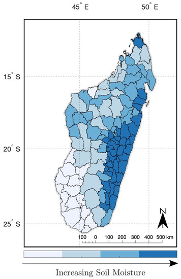
Figure 4.
Districts are grouped into four climate regions based on the average soil moisture within the district from 2010 to 2017. We refer to these regions from low to high soil moisture as “arid”, “semi-arid”, “semi-wet”, and “wet”.
Production also varies substantially between the four regions, with the arid and semi-arid regions producing less relative to the semi-wet and wet regions (Table 1). More specifically, the sum of production in arid and semi-arid regions accounts for 23% of total rice production, 35% of total cassava production, 33% of total maize production, and 39% of total sweet potato production. For completeness, we also evaluate variations in production at the national-scale by relating national variations in production to anomalies in national-average soil moisture.

Table 1.
The average production (in tonnes × 10) of rice, cassava, maize, and sweet potatoes in each climate-zone and nationally from 2010–2017.
2.3. Relating Variations in Soil Moisture to Production
2.3.1. Yield and Soil Moisture Time Series
To relate soil moisture conditions to interannual variations in yearly crop production, we temporally average the soil moisture () at each 0.05-degree grid box according to each of the four different calendars. The production reported for each year is assumed to represent the crop harvested in that year, though it may be planted and grown in the year prior. Both production and are detrended from 2010 to 2017 using a linear regression model. Trends are removed at the lowest resolved level, or at each 0.05-degree grid box for and the district level for crop production. Detrending the data allows for better isolating weather influences, rather than multi-year trends that are often associated with changes in technology, farming practices, or other land-use changes [43].
District-scale soil moisture averages are obtained by averaging across grid boxes that have crop-specific fractions greater than 0.001. Note that many grid boxes have small crop fractions; for example, 41% of all grid boxes with non-zero rice production have fractions between 0.01 and 0.001. Results are generally consistent if the minimum crop fraction is raised to 0.01 or 0.025 (Tables S8 and S9). Regional-scale soil moisture is obtained by averaging across districts using weights that are proportional to production. Other plausible changes to the crop-production and weighting procedures have negligible influence on the results (Table S10).
2.3.2. Scaling
After spatial and temporal averaging to match the scale of the production data, anomalies in () are linearly scaled to anomalies in crop production (),
where a is a sensitivity coefficient and b is a constant offset. We assess the strength of the relationship between and using the Pearson correlation coefficient (r). Confidence intervals for r are estimated by bootstrapping the observations with samples (Table 2 for 90% confidence intervals; Table S1 for 95% confidence intervals). The magnitude of a is difficult to compare across crops and regions because it reflects both the sensitivity to soil moisture and magnitude in production variability, although its sign is useful for distinguishing between greater explanatory power associated with anomalies toward saturated or drought conditions.
Table 2.
The correlation (r) between and for each crop across four climate-zones and nationally. Values in parentheses represent 90% confidence intervals. We evaluate Equation (1) using soil anomalies that are based on planting and harvesting dates ( and ) and based on NDVI, with a fixed length of eight months () and an optimal length (). The optimal lengths are shown in (Table 3).
We assess the performance of Equation (1) using an out-of-sample approach in order to aid assessment of whether Equation (1) is overfit given the small number of years available. The coefficient of determination () is determined out-of-sample by developing the predicted time series through estimating a and b after excluding one year of data and predicting the anomaly in crop production for the excluded year using the estimated a and b coefficients. The excluded year is sequentially shifted until a full time series is predicted. To compute out-of-sample values (), the normalized residual sum of squares is calculated from these out-of-sample predictions (Table S2). Values of are often within 20% of , indicating that the correspondence that we obtain between predictions and observations is not heavily influenced by overfitting. Note that negative values of can occur because it is estimated out-of-sample and, unlike in-sample , the out-of-sample residual sum of squares can be larger than the total sum of squares. The is negative when predictions fit worse than would be the case if simply using the mean of the observations.
3. Results
There are numerous combinations of calendars and crop distribution maps that can be used to evaluate the relationship between soil moisture and production, and these can be applied over a range of spatial averages, using district, regional (Figure 4), or national data. We compare various combinations of calendars (C1–C4), maps (crop-specific vs. generic), and spatial averages of results to those that correspond to regional-scale averages using crop-specific distribution maps and C3, or the NDVI-based growing season with a fixed eight-month growing season, as a baseline (Table 2). In this baseline case, variations in rice production are well captured across each of the four regional clusters and nationally, with all r values significantly greater than zero at the 90% confidence level. Soil moisture anomalies using C3 () also well track variations in cassava in the arid region (r = 0.88; 90% CI: 0.67–0.96) and at the national scale (r = 0.92; 90% CI: 0.73–0.98). In the semi-wet region, correlations between cassava production and soil moisture are lower (r = 0.75; 90% CI: 0.21–0.94), while there is no correspondence in the semi-arid or semi-wet, i.e., the confidence intervals bound zero. Similar patterns are found for maize, with predictive power in the arid region (r = 0.70; 90% CI: 0.34–0.90) and nationally (r = 0.93; 90% CI: 0.70–0.99), but insignificant correlations elsewhere. Unlike rice, cassava, and maize, though, we find no correspondence between variations in sweet potato production and in any region, although the national-level r-value is 0.68 (90% CI: 0.04–0.94).
Using crop calendars that are based on mean planting and harvesting dates (C1 and C2) give results with less skill relative to C3 (Table 2). For example, C1 and C2 both show insignificant relationships in the wet region for rice, with the 90% confidence intervals bounding zero, while C3 and C4 show significant relationships (C3: r = 0.85, 90% CI: 0.19–0.95; C4: r = 0.93, 90% CI: 0.7–0.96). It is important to note the wide confidence interval for C3, though, which is partially a result of the short time interval of eight years. At the national-level, C1 gives an insignificant relationship between soil moisture and rice production, whereas C2, C3, and C4 all give significant relationships. Furthermore, C2 gives an insignificant relationship for maize and sweet potato, while C1 gives significant relationships. As noted, C3 and C4 both give significant relationships for all four crops nationally.
Optimizing the growing season length for each climate-zone and crop leads to small improvements in r for rice, cassava, and maize and large improvements in r for sweet potatoes (C4, Table 2). An already strong relationship between rice and is slightly improved by lengthening the annual interval over which soil moisture is averaged from 8 months to 9, 11, or 12 months (Figure 5; Table 3). The r between sweet potato and soil moisture increases from values that are indistinguishable from zero to r = 0.93 (90% CI: 0.82–0.99) in the arid region and r = −0.93 (90% CI: −0.99–−0.6 ) in the semi-arid region by decreasing the interval over which soil moisture is averaged from 8 to only 2 and 1 months, respectively. These short intervals may be interpreted as the months in which variations in soil moisture most influence production. The fact that the inferred relationship between sweet potato and in the semi-arid region is negative suggests that wet conditions adversely affect production. As the length of the averaging period increases, the correlation and sensitivity coefficient become positive, indicating that an overall reduction in water availability limits production (Figure S15).
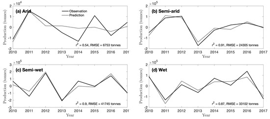
Figure 5.
Observations and predictions of rice production anomalies (tonnes) in the (a) arid, (b) semi-arid, (c) semi-wet, and (d) wet climate-zones. Note that the y-axis of each subplot has a different scale. Anomalies in production are computed as a deviation from a least-squares fit linear trend (see Table 1 for the average total production in each region). Predictions are made using the optimal growing season length () following Equation (1). Observations are plotted with a solid line and predictions with a dotted line. See Figures S12–S14 for analogous plots for maize, cassava, and sweet potatoes.
Table 3.
The optimal number of months for the soil-moisture-averaging period for each crop over the four climate-zones and nationally. This optimal length is determined by maximizing the absolute correlation coefficient (r) between variations in soil moisture and production. The start of the averaging period varies within the regions based on the minimum NDVI of each 0.05-degree grid box.
Comparable correlations are obtained if crop predictions are made using the Global Food Security-Support Analysis Data (Table S3), instead of the crop-specific maps that we rely upon from [40]. Using the MCD12C1v006 dynamic cropland map [38], though, leads to worse predictions at both the regional and national-scales relative to the crop specific maps and the GFSAD30 data product (Table S4).
4. Discussion
There are three major components to our prediction involving climate variables, crop calendars, and crop maps.
We focus on resolving the response of crop-specific production to soil moisture, rather than variables such as temperature and precipitation, because of the recent droughts in Madagascar [6,7,8] and the generally strong relationship between water availability and both dry and flooded rice production [21]. Rice in Madagascar is mainly grown in irrigated lowlands (66% of rice area), though rainfed lowland rice (27%) and upland rice (7%; often referred to as “tanety”) are important cultivation methods for many farmers [44]. The sensitivity of rice production to soil moisture likely depends on cultivation method but, without maps of cultivation practices, making such distinctions is not currently feasible. Considering both rainfed and irrigated rice, water stress is estimated to account for between 10–31% of the rice yield gap in Sub-Saharan Africa [45]. In a review of constraints on crop production in Sub-Saharan Africa [46], researchers found that water stress is the leading environmental driver for reductions in rice production, but that water stress is comparable or relatively less important than biotic and nutrient constraints for cassava, maize, and sweet potato. This ranking accords with the higher Pearson correlation values for rice than other crops, averaged across climate-zones for each calendar (Table 2).
Previous studies have found temperature and precipitation to be relevant explanatory variables when estimating crop production in other agricultural systems, including Mozambique (e.g., [47]), Malawi (e.g., [48]), and across Sub-Saharan Africa (excluding Madagascar) (e.g., [49,50]). It is important to recognize that the influence of both temperature and precipitation is partially reflected in the remotely sensed soil moisture signal at synoptic and inter-annual time scales due to its physical coupling with temperature and precipitation [51]. Disentangling these drivers would benefit from a more-refined analysis wherein variability in temperature and water availability was assessed at daily timescales, but which is beyond the scope of the present analysis.
When relating remotely sensed soil moisture to variations in production, we find that the strength of the relationship is highly dependent on the months of the year over which soil moisture is averaged. Given the spatial heterogeneity in climate across Madagascar (Figure 1), it can be assumed that this temporal interval also varies spatially, as well as by crop because different crops have distinct growing periods and sensitives to water stress. Soil moisture measured over the intervals defined in calendars C1 and C2 generally capture less production variability than soil moisture averaged over the more-detailed NDVI-based calendars (C3 and C4). Interestingly, the correlation between production and soil moisture is not improved by the spatial heterogeneities introduced by C2 relative to that of C1. Though C1 and C2 have similar planting times, they differ widely with respect to their harvesting dates for rice (Figure 3e,f) as well as planting and harvesting dates for sweet potatoes (Figure S6).
Averaging soil moisture from the minimum in NDVI over an 8-month period (C3) performs relatively better than either C1 or C2. Because NDVI observations contain a mixture of signals from natural vegetation, agriculture, and other activities, this calendar represents general environmental variability. An important question is the degree to which natural vegetation, which is typically perennial, versus agricultural activity, often involving annuals, undergoes a similar cycle of greening and drying. This question might be further pursued by looking for differences in seasonality depending on the mixture of crops and natural vegetation.
We refine C3 by finding the optimal number of months after the minimum in NDVI that best correlates with variations in production, giving C4. C4 represents the period in which soil moisture most influences production, which is potentially distinct from a growing season. Correlations between soil moisture and production under C4 are almost all significantly different than zero for the different crop-climate combinations (13 of the 16; Table 2). The optimal number of months can be short (Table 3), such as in the case of sweet potatoes in the semi-arid region, which exhibits a strong anti-correlation between soil moisture and production during the month of minimum NDVI. The decline associated with wet conditions may also be associated with flooding, possibly as a result of cyclones that primarily affect the east and west coasts and the northwestern region of Madagascar [52]. A future model could incorporate the influences of both wet and dry soil moisture conditions on different stages of sweet potato production, though we refrain from fitting a more-detailed model at this stage on account of the limited data. It may also be the case that crop substitution is an important factor in production anomalies, but analysis of which requires accurate estimates of the farmland devoted to different crops.
The correlations between soil moisture and crop production are comparable when using the Global Food Security-Support Analysis cropland maps (Table S3) and the crop-specific maps [40]. There are three possible reasons for this similarity. First, soil moisture anomalies within clusters are similar to one another. The average pairwise correlation between the grid box time series of 8-month seasonal average anomalies in soil moisture within clusters is 0.63 for the arid region, 0.30 for the semi-arid region, 0.21 for the semi-wet region, and 0.55 for the wet region (when all grid boxes, regardless of crop fraction, are included). Second, soil moisture observations at the grid box scale are noisy, and averaging more locations together, insomuch as the underlying soil moisture anomaly signal is consistent across boxes, leads to a higher signal to noise. When the minimum crop fraction is set to 0.001, GFSAD30 involves averaging 53% of the grid boxes across Madagascar, whereas the crop specific distribution maps for rice, cassava, maize, and sweet potato correspond with 71%, 47%, 37%, and 19%, respectively. If the minimum crop fraction is set to 0.025, GFSAD30 involves averaging 32% of the grid boxes across Madagascar, whereas the crop specific distribution maps for rice, cassava, maize, and sweet potato correspond with 20%, 5%, <1%, and <1%, respectively. Finally, the location of specific crop production is uncertain and includes year-to-year variability that is not accounted for in the crop-specific maps from [37] or GFSAD30.
In contrast, using the generic cropland map from MCD12C1v006 (Table S4) leads to lower correlations between soil moisture and crop production relative to using the GFSAD30 cropland map (Table S3). The correlation between soil moisture and national-scale production of rice for C3 under MCD12C1v006 is 0.8 (0.21–0.98), whereas under GFSAD30 it is 0.86 (90% CI: 0.41–0.96). Although the MCD12C1v006 and GFSAD30 datasets are meant to both represent the spatial distribution of croplands, there are notable differences across Madagascar (Figure S3) that contribute to the large differences in skill. Our result indirectly suggests that cropland areas from GFSAD30 are more representative of actual agricultural areas in Madagascar compared to MCD12C1v006, although a more direct analysis would involve land-use validation datasets that are beyond the scope of this study. Future work may also involve incorporating dynamic harvested area maps, as there has been considerable deforestation, for example, in Eastern Madagascar associated with swidden agricultural practices (“tavy”) [53]. According to the Global Forest Watch, shifting agriculture is the dominant driver of tree cover loss in Madagascar, accounting for over 96% of the total 4.13 Mha tree cover loss from 2001 to 2020 ([54]; accessed through Global Forest Watch on 2 January 2022, www.globalforestwatch.org).
Although a district-level analysis would be ideal, as it is the most well-resolved, we find that the district-level relationships between production and water availability are too noisy for interpretation (Figure S16), likely due to errors in reported production data, crop calendars, and crop maps but whose influence was reduced by averaging over larger climate-zones. Errors in the reported production data, for example, may degrade the correspondence between production and soil moisture [55]. Regional analyses by climate-zones allows for important spatial heterogeneity to be resolved, though, that is not apparent in nationally reported statistics or predictions. For example, the anomaly in national rice production in 2011 was −1.7 × 10 tonnes, but this anomaly was the small residual of strong positive anomalies in rice production in arid and semi-arid regions (Figure 5a,b) and negative anomalies in wet and semi-wet regions (Figure 5c,d). Reported regional variations in rice production are all well captured by the NDVI-based calendars (C3 and C4). Since the majority of Malagasy people depend on local food sources, particularly in the South during the wet-season when roads are difficult to travel [56], resolving these regional differences is of high priority.
5. Conclusions
Our results provide a basis for understanding and predicting staple food production in Madagascar using satellite-based soil moisture observations. The available data suggests that anomalies in rice production can be well explained across all climate-zones using remotely-sensed soil moisture when the relevant time of year is isolated as the 8-months after the minimum in NDVI (C3). Furthermore, optimizing the length of the averaging period increases the correlations substantially (C4) for sweet potato, though this comes with the strong caveat that the calendar may overfit the eight years of observations.
We intend for this work to serve as a proof of concept that remotely sensed soil moisture can be related to regional Malagasy crop statistics, even though there remains large uncertainties in crop calendars and distribution maps. Furthermore, accounting for additional growth determinants including soils (e.g., [57]), temperature (e.g., [50]), storms (e.g., [5]) that are understood as important controls in Madagascar and elsewhere will be useful insomuch as sufficient additional observational and theoretical constraints can be incorporated into future analyses. This modeling framework can also be applied in other developing nations, though the skill would need to be assessed in detail for each application. Given the severity of recent droughts in Madagascar and their associated impacts on food insecurity and severe malnutrition, we hope this study encourages future work using soil moisture predictions to forecast near and long-term changes in Malagasy agricultural production so that future droughts do not incur similar damage.
Supplementary Materials
The following are available online at https://www.mdpi.com/article/10.3390/rs14051223/s1, Figures S1–S16, Tables S1–S10, Supplementary Data on FAO Calendars.
Author Contributions
Conceptualization, A.J.R., C.G. and P.H.; methodology, A.J.R. and P.H.; formal analysis, A.J.R.; data curation, A.J.R.; writing—original draft preparation, A.J.R.; writing—review and editing, A.J.R., C.G. and P.H.; funding acquisition, P.H. and C.G. All authors have read and agreed to the published version of the manuscript.
Funding
Support was provided by the United States Agency for International Development (Grant No. AID-FFP-A-14-00008) and implemented by Catholic Relief Services. Financial support was also provided by the Ren Che Foundation (C.G.).
Data Availability Statement
All data products used in this study are publicly available except for the district-level crop production data, which can be obtained upon request.
Acknowledgments
Joceline Solonitompoarinony of the Malagasy Ministry of Agriculture and Livestock organized and provided district-level data for us.
Conflicts of Interest
The authors declare no conflict of interest.
References
- INSTAT; UNICEF. Multiple Indicator Cluster Survey–MICS Madagascar, 2018, Final Report; Technical Report; INSTAT and UNICEF: Antananarivo, Madagascar, 2019. [Google Scholar]
- FAO. Madagascar–Impact of Early Warning Early Action; Technical Report; FAO: Rome, Italy, 2019. [Google Scholar]
- Harvey, C.A.; Rakotobe, Z.L.; Rao, N.S.; Dave, R.; Razafimahatratra, H.; Rabarijohn, R.H.; Rajaofara, H.; MacKinnon, J.L. Extreme vulnerability of smallholder farmers to agricultural risks and climate change in Madagascar. Philos. Trans. R. Soc. Biol. Sci. 2014, 369, 20130089. [Google Scholar] [CrossRef]
- Golden, C.D.; Gephart, J.A.; Eurich, J.G.; McCauley, D.J.; Sharp, M.K.; Andrew, N.L.; Seto, K.L. Social-ecological traps link food systems to nutritional outcomes. Glob. Food Secur. 2021, 30, 100561. [Google Scholar] [CrossRef]
- Rakotobe, Z.; Harvey, C.A.; Rao, N.S.; Dave, R.; Rakotondravelo, J.C.; Randrianarisoa, J.; Ramanahadray, S.; Andriambolantsoa, R.; Razafimahatratra, H.; Rabarijohn, R.H.; et al. Strategies of smallholder farmers for coping with the impacts of cyclones: A case study from Madagascar. Int. J. Disaster Risk Reduct. 2016, 17, 114–122. [Google Scholar] [CrossRef]
- FAO. Madagascar–Response Overview—May 2021; Technical Report; FAO: Rome, Italy, 2021. [Google Scholar]
- FAO. GIEWS Update–Madagascar, February 2021; Technical Report; FAO: Rome, Italy, 2021. [Google Scholar]
- WFP. WFP Madagascar Country Brief (May 2021); Technical Report; World Food Programme: Rome, Italy, 2021. [Google Scholar]
- Makoni, M. Southern Madagascar faces “shocking” lack of food. Lancet 2021, 397, 2239. [Google Scholar] [CrossRef]
- Minten, B.; Barrett, C.B. Agricultural Technology, Productivity, and Poverty in Madagascar. World Dev. 2008, 36, 797–822. [Google Scholar] [CrossRef]
- UNDESA. World Urbanization Prospects: The 2018 Revision; United Nations: New York, NY, USA, 2019. [Google Scholar] [CrossRef]
- Schauberger, B.; Jägermeyr, J.; Gornott, C. A systematic review of local to regional yield forecasting approaches and frequently used data resources. Eur. J. Agron. 2020, 120, 126153. [Google Scholar] [CrossRef]
- Weiskopf, S.; Cushing, J.A.; Morelli, T.L.; Bonnie, M. Climate change risks and adaptation options for Madagascar. Ecol. Soc. 2021, 26, 36. [Google Scholar] [CrossRef]
- Karthikeyan, L.; Chawla, I.; Mishra, A.K. A review of remote sensing applications in agriculture for food security: Crop growth and yield, irrigation, and crop losses. J. Hydrol. 2020, 586, 124905. [Google Scholar] [CrossRef]
- Weiss, M.; Jacob, F.; Duveiller, G. Remote sensing for agricultural applications: A meta-review. Remote Sens. Environ. 2020, 236, 111402. [Google Scholar] [CrossRef]
- Rembold, F.; Atzberger, C.; Savin, I.; Rojas, O. Using Low Resolution Satellite Imagery for Yield Prediction and Yield Anomaly Detection. Remote Sens. 2013, 5, 1704–1733. [Google Scholar] [CrossRef]
- Smith, M.R.; Micha, R.; Golden, C.D.; Mozaffarian, D.; Myers, S.S. Global Expanded Nutrient Supply (GENuS) Model: A New Method for Estimating the Global Dietary Supply of Nutrients. PLoS ONE 2016, 11, e0146976. [Google Scholar] [CrossRef] [PubMed]
- MacIntosh, T. Growing Relations: An Ethnographic Study on Rice, Vanilla, and Yams in Madagascar. Ph.D. Thesis, The University of Western Ontario, London, ON, Canada, 2020. [Google Scholar]
- Golden, C.D.; Vaitla, B.; Ravaoliny, L.; Vonona, M.A.; Anjaranirina, E.G.; Randriamady, H.J.; Glahn, R.P.; Guth, S.E.; Fernald, L.C.; Myers, S.S. Seasonal trends of nutrient intake in rainforest communities of north-eastern Madagascar. Public Health Nutr. 2019, 22, 2200–2209. [Google Scholar] [CrossRef] [PubMed]
- Dostie, B.; Haggblade, S.; Randriamamonjy, J. Seasonal poverty in Madagascar: Magnitude and solutions. Food Policy 2002, 27, 493–518. [Google Scholar] [CrossRef]
- Bouman, B.; Humphreys, E.; Tuong, T.P.; Barker, R. Rice and water. Adv. Agron. 2007, 92, 187–237. [Google Scholar] [CrossRef]
- Randriamarolaza, L.Y.A.; Aguilar, E.; Skrynyk, O.; Vicente-Serrano, S.M.; Domínguez-Castro, F. Indices for daily temperature and precipitation in Madagascar, based on quality-controlled and homogenized data, 1950–2018. Int. J. Climatol. 2022, 42, 265–288. [Google Scholar] [CrossRef]
- Rigden, A.J.; Ongoma, V.; Huybers, P. Kenyan tea is made with heat and water: How will climate change influence its yield? Environ. Res. Lett. 2020, 15, 044003. [Google Scholar] [CrossRef]
- Rigden, A.J.; Mueller, N.D.; Holbrook, N.M.; Pillai, N.; Huybers, P. Combined influence of soil moisture and atmospheric evaporative demand is important for accurately predicting US maize yields. Nat. Food 2020, 1, 127–133. [Google Scholar] [CrossRef]
- Lesk, C.; Rowhani, P.; Ramankutty, N. Influence of extreme weather disasters on global crop production. Nature 2016, 529, 84–87. [Google Scholar] [CrossRef]
- ICTSD-IPC. ICTSD-IPC Platform on Climate Change, Agriculture and Trade: Considerations for Policymakers; Technical Report; ICTSD and IPC: Geneva, Switzerland, 2009. [Google Scholar]
- Oldeman, L.R. Technical Paper 21: An Agroclimatic Characterization of Madagascar; Technical Report; ISRIC: Wageningen, The Netherlands, 1990. [Google Scholar]
- Dunham, A.E.; Erhart, E.M.; Wright, P.C. Global climate cycles and cyclones: Consequences for rainfall patterns and lemur reproduction in southeastern Madagascar. Glob. Chang. Biol. 2011, 17, 219–227. [Google Scholar] [CrossRef]
- Arivelo, T.A.; Lin, Y.L. Climatology of Heavy Orographic Rainfall Induced by Tropical Cyclones over Madagascar: From Synoptic to Mesoscale Perspectives. Earth Sci. Res. 2016, 5, 132. [Google Scholar] [CrossRef]
- Didan, K. MOD13C2 MODIS/Terra Vegetation Indices Monthly L3 Global 0.05Deg CMG V006 [Data set]. In NASA EOSDIS Land Processes DAAC; 2015. Available online: https://lpdaac.usgs.gov/products/mod13c2v006/ (accessed on 22 December 2021). [CrossRef]
- Johnson, D.M.; Rosales, A.; Mueller, R.; Reynolds, C.; Frantz, R.; Anyamba, A.; Pak, E.; Tucker, C. USA Crop Yield Estimation with MODIS NDVI: Are Remotely Sensed Models Better than Simple Trend Analyses? Remote Sens. 2021, 13, 4227. [Google Scholar] [CrossRef]
- Ozdogan, M.; Yang, Y.; Allez, G.; Cervantes, C. Remote Sensing of Irrigated Agriculture: Opportunities and Challenges. Remote Sens. 2010, 2, 2274–2304. [Google Scholar] [CrossRef]
- Boschetti, M.; Stroppiana, D.; Brivio, P.A.; Bocchi, S. Multi-year monitoring of rice crop phenology through time series analysis of MODIS images. Int. J. Remote Sens. 2009, 30, 4643–4662. [Google Scholar] [CrossRef]
- Dorigo, W.; Wagner, W.; Albergel, C.; Albrecht, F.; Balsamo, G.; Brocca, L.; Chung, D.; Ertl, M.; Forkel, M.; Gruber, A.; et al. ESA CCI Soil Moisture for improved Earth system understanding: State-of-the art and future directions. Remote Sens. Environ. 2017, 203, 185–215. [Google Scholar] [CrossRef]
- Liu, Y.Y.; Dorigo, W.A.; Parinussa, R.M.; De Jeu, R.A.M.; Wagner, W.; McCabe, M.F.; Evans, J.P.; van Dijk, A.I.J.M. Trend-preserving blending of passive and active microwave soil moisture retrievals. Remote Sens. Environ. 2012, 123, 280–297. [Google Scholar] [CrossRef]
- Gruber, A.; Dorigo, W.A.; Crow, W.T.; Wagner, W. Triple Collocation-Based Merging of Satellite Soil Moisture Retrievals. IEEE Trans. Geosci. Remote Sens. 2017, 55, 6780–6792. [Google Scholar] [CrossRef]
- Monfreda, C.; Ramankutty, N.; Foley, J.A. Farming the planet: 2. Geographic distribution of crop areas, yields, physiological types, and net primary production in the year 2000. Glob. Biogeochem. Cycles 2008, 22, GB1022. [Google Scholar] [CrossRef]
- Friedl, M.; Sulla-Menashe, D. MCD12C1 MODIS/Terra+Aqua Land Cover Type Yearly L3 Global 0.05Deg CMG V006 [Data set]. In NASA EOSDIS Land Processes DAAC; 2015. Available online: https://lpdaac.usgs.gov/products/mcd12c1v006/ (accessed on 22 December 2021). [CrossRef]
- Xiong, J.; Thenkabail, P.; Tilton, J.; Gumma, M.; Teluguntla, P.; Congalton, R.; Yadav, K.; Dungan, J.; Oliphant, A.; Poehnelt, J.; et al. NASA Making Earth System Data Records for Use in Research Environments (MEaSUREs) Global Food Security-support Analysis Data (GFSAD) Cropland Extent 2015 Africa 30 m V001 [Data set]. In NASA EOSDIS Land Processes DAAC; 2017. Available online: https://lpdaac.usgs.gov/products/gfsad30afcev001/ (accessed on 22 December 2021). [CrossRef]
- Sacks, W.J.; Deryng, D.; Foley, J.A.; Ramankutty, N. Crop planting dates: An analysis of global patterns. Glob. Ecol. Biogeogr. 2010, 19, 607–620. [Google Scholar] [CrossRef]
- Franke, J.A.; Müller, C.; Elliott, J.; Ruane, A.C.; Jägermeyr, J.; Balkovic, J.; Ciais, P.; Dury, M.; Falloon, P.D.; Folberth, C.; et al. The GGCMI Phase 2 experiment: Global gridded crop model simulations under uniform changes in CO2, temperature, water, and nitrogen levels (protocol version 1.0). Geosci. Model Dev. 2020, 13, 2315–2336. [Google Scholar] [CrossRef]
- Beck, H.E.; Zimmermann, N.E.; McVicar, T.R.; Vergopolan, N.; Berg, A.; Wood, E.F. Present and future Köppen-Geiger climate classification maps at 1-km resolution. Sci. Data 2018, 5, 180214. [Google Scholar] [CrossRef]
- Lobell, D.B.; Schlenker, W.; Costa-Roberts, J. Climate Trends and Global Crop Production Since 1980. Science 2011, 333, 616–620. [Google Scholar] [CrossRef] [PubMed]
- Diagne, A.; Amovin-Assagba, E.; Futakuchi, K.; Wopereis, M.C.S. Estimation of cultivated areas, number of farming households and yield of major rice-growing environments in Africa. In Realizing Africa’s Rice Promise; CAB International: Wallingford, UK, 2013; pp. 35–45. [Google Scholar] [CrossRef]
- Waddington, S.R.; Li, X.; Dixon, J.; Hyman, G.; De Vicente, M.C. Getting the focus right: Production constraints for six major food crops in Asian and African farming systems. Food Secur. 2010, 2, 27–48. [Google Scholar] [CrossRef]
- Reynolds, T.W.; Waddington, S.R.; Anderson, C.L.; Chew, A.; True, Z.; Cullen, A. Environmental impacts and constraints associated with the production of major food crops in Sub-Saharan Africa and South Asia. Food Secur. 2015, 7, 795–822. [Google Scholar] [CrossRef]
- Harrison, L.; Michaelsen, J.; Funk, C.; Husak, G. Effects of temperature changes on maize production in Mozambique. Clim. Res. 2011, 46, 211–222. [Google Scholar] [CrossRef]
- McCarthy, N.; Kilic, T.; Brubaker, J.; Murray, S.; de la Fuente, A. Droughts and floods in Malawi: Impacts on crop production and the performance of sustainable land management practices under weather extremes. Environ. Dev. Econ. 2021, 26, 432–449. [Google Scholar] [CrossRef]
- Hoffman, A.L.; Kemanian, A.R.; Forest, C.E. Analysis of climate signals in the crop yield record of sub-Saharan Africa. Glob. Chang. Biol. 2018, 24, 143–157. [Google Scholar] [CrossRef]
- Lobell, D.B.; Bänziger, M.; Magorokosho, C.; Vivek, B. Nonlinear heat effects on African maize as evidenced by historical yield trials. Nat. Clim. Chang. 2011, 1, 42–45. [Google Scholar] [CrossRef]
- Seneviratne, S.I.; Corti, T.; Davin, E.L.; Hirschi, M.; Jaeger, E.B.; Lehner, I.; Orlowsky, B.; Teuling, A.J. Investigating soil moisture–climate interactions in a changing climate: A review. Earth Sci. Rev. 2010, 99, 125–161. [Google Scholar] [CrossRef]
- Rakotoarison, N.; Raholijao, N.; Razafindramavo, L.M.; Rakotomavo, Z.A.P.H.; Rakotoarisoa, A.; Guillemot, J.S.; Randriamialisoa, Z.J.; Mafilaza, V.; Ramiandrisoa, V.A.M.P.; Rajaonarivony, R.; et al. Assessment of Risk, Vulnerability and Adaptation to Climate Change by the Health Sector in Madagascar. Int. J. Environ. Res. Public Health 2018, 15, 2643. [Google Scholar] [CrossRef]
- Styger, E.; Rakotondramasy, H.M.; Pfeffer, M.J.; Fernandes, E.C.; Bates, D.M. Influence of slash-and-burn farming practices on fallow succession and land degradation in the rainforest region of Madagascar. Agric. Ecosyst. Environ. 2007, 119, 257–269. [Google Scholar] [CrossRef]
- Curtis, P.G.; Slay, C.M.; Harris, N.L.; Tyukavina, A.; Hansen, M.C. Classifying drivers of global forest loss. Science 2018, 361, 1108–1111. [Google Scholar] [CrossRef] [PubMed]
- Lobell, D.B.; Di Tommaso, S.; Burke, M.; Kilic, T. Twice Is Nice: The Benefits of Two Ground Measures for Evaluating the Accuracy of Satellite-Based Sustainability Estimates. Remote Sens. 2021, 13, 3160. [Google Scholar] [CrossRef]
- USAID. Climate Risks in Food for Peace Geographies: Madagascar; Technical Report; USAID: Washington, DC, USA, 2019.
- Tsujimoto, Y.; Horie, T.; Randriamihary, H.; Shiraiwa, T.; Homma, K. Soil management: The key factors for higher productivity in the fields utilizing the system of rice intensification (SRI) in the central highland of Madagascar. Agric. Syst. 2009, 100, 61–71. [Google Scholar] [CrossRef]
Publisher’s Note: MDPI stays neutral with regard to jurisdictional claims in published maps and institutional affiliations. |
© 2022 by the authors. Licensee MDPI, Basel, Switzerland. This article is an open access article distributed under the terms and conditions of the Creative Commons Attribution (CC BY) license (https://creativecommons.org/licenses/by/4.0/).