Improved k-NN Mapping of Forest Attributes in Northern Canada Using Spaceborne L-Band SAR, Multispectral and LiDAR Data

Abstract

Satellite forest inventories are the only feasible way to map Canada’s vast, remote forest regions, such as those in the Northwest Territories (NWT). A method used to create such inventories is the k-nearest neighbour (k-NN) algorithm, which spatially extends information from forest inventory (FI) plots to the entire forest land base using wall-to-wall features typically derived from Landsat data. However, the benefits of integrating L-band synthetic aperture radar (SAR) data, strongly correlated to forest biomass, have not been assessed for Canadian northern boreal forests. Here we describe an optimized multivariate k-NN implementation of a 151,700 km² area in southern NWT that included ca. 2007 Landsat and dual-polarized Phased Array type L-band SAR (PALSAR) data on board the Advanced Land Observing Satellite (ALOS). Five forest attributes were mapped at 30 m cells: stand height, crown closure, stand/total volume and aboveground biomass (AGB). We assessed accuracy gains compared to Landsat-based maps. To circumvent the scarcity of FI plots, we used 3600 footprints from the Geoscience Laser Altimeter System (GLAS) as surrogate FI plots, where forest attributes were estimated using Light Detection and Ranging (LiDAR) metrics as predictors. After optimization, k-NN predicted forest attribute values for each pixel as the average of the 4 nearest (k = 4) surrogate FI plots within the Euclidian space of 9 best features (selected among 6 PALSAR, 10 Landsat, and 6 environmental features). Accuracy comparisons were based on 31 National Forest Inventory ground plots and over 1 million airborne LiDAR plots. Maps that included PALSAR HV backscatter resulted in forest attribute predictions with higher goodness of fit (adj. R²), lower percent mean error (ME%), and percent root mean square error (RMSE%), and lower underestimation for larger attribute values. Predictions were most accurate for conifer stand height (RMSE% = 32.1%, adj. R² = 0.58) and AGB (RMSE% = 47.8%, adj. R² = 0.74), which is much more abundant in the area than mixedwood or broadleaf. Our study demonstrates that optimizing k-NN parameters and feature space, including PALSAR, Landsat, and environmental variables, is a viable approach for inventory mapping of the northern boreal forest regions of Canada.

1. Introduction

Information on forest composition and structure is necessary to support forest ecosystem management [1,2]. In Canada, this information is typically captured in the form of forest inventory maps derived from the interpretation of aerial photographs [3,4]. In the Northwest Territories (NWT), Canada, however, it is impractical to undertake a conventional forest inventory over its vast, widely distributed ≈ 40 million ha of forest landscape [5]. As a result, there has been considerable interest in exploring the use of remote sensing at various spatial scales in boreal forests of Canada, including the NWT [6,7,8].

The application of remote sensing for estimating and mapping forest inventory attributes such as stand height, crown closure, timber volume, and aboveground biomass (AGB) has evolved considerably. This is in part due to the rapid development of airborne and satellite sensors operating at different spatial and temporal scales and their methods of analysis, which can supplement or enhance forest inventory programs [2,9,10]. In particular, small-footprint airborne light detection and ranging (LiDAR: also known as airborne laser scanning, or ALS) has proven successful as a sampling tool to estimate and map vertically distributed attributes such as canopy height [11,12,13]. However, ALS is usually not suitable for mapping large areas because of challenges from large data volumes and acquisition logistics [13]. The vintage of ALS data is also a consideration, as the timing of ALS aerial survey and in-situ field measurements should be similar to ensure the data are suitable for calibration and are representative of the forest landscape to be mapped [14].

Andersen et al. [15] first reported an approach to predict forest attributes based on a multi-level spatial modelling framework. Such an approach, combining forest inventory (FI) plots, ALS data, satellite imagery, and other spatial datasets, is particularly well suited for inventories of remote regions where logistical difficulties and high costs limit the number of FI plots that can be established [15,16]. It has also been applied to map large regions within and across the circumboreal forest [8,17].

Mapping forest attributes over large areas requires a large reference dataset consisting of numerous FI plots distributed throughout the area to be mapped. Such a dense network of FI plots only exists in a few countries, such as Finland [18] and the United States [19]. When there is an insufficient number of FI plots, those available can be used to develop models that relate field measurements to metrics generated from ALS datasets [12,20] and further scaled to satellite waveform LiDAR, which has been shown to strongly correlate with ALS data [21]. For example, global observations from the Geoscience Laser Altimeter System (GLAS) [22] onboard the Ice, Cloud, and land Elevation Satellite (ICESat) were used to estimate forest attributes such as canopy height and AGB [13,23,24]. Generating multi-level models of forest attributes between FI plots and ALS, and then between ALS and GLAS, offers the opportunity to create a reference dataset for spatial prediction that is denser and more spatially distributed than datasets generated from FI plots or ALS data alone.

In the NWT, the scarcity of ground FI plots and ALS data became the impetus to scale relationships between these data to GLAS footprints, where the latter served as surrogate FI plots that were later scaled up to the entire forest land base using Landsat and environmental features [7]. While there are several algorithms suited for this task [2], we chose the k-nearest neighbour (k-NN) machine learning algorithm because of its non-parametric nature, ease of use and ability for simultaneous predictions of multiple dependent variables [25,26]. Its expanding use over the last decade has been documented for a wide variety of forestry applications, including forest inventory mapping based on remotely sensed data and FI plots [26,27,28].

This approach, presented in Mahoney et al. [7], is the foundation for the Multisource Vegetation Inventory (MVI), a joint project of Natural Resources Canada, Canadian Forest Service and the Forest Management Division of the Government of NWT [5]. One of the recommendations from Mahoney et al. [7] was to evaluate the addition of Synthetic Aperture Radar (SAR) data for improving spatial predictions of forest attributes. In particular, L-band SAR dual-polarized (HH, HV) backscatter datasets from the Phased Array type L-band Synthetic Aperture Radar (PALSAR) on board the Advanced Land Observing Satellite missions (ALOS-1 [29] and ALOS-2) has been found to strongly correlate to forest biomass and related structural attributes across multiple forest biomes as summarized in [30]. In particular, the HV-polarized backscatter from PALSAR has been found the best predictor of biomass and volume in many forest biomes [30], including boreal forests in Sweden, Alaska, and Siberia [31,32,33].

Over the last decade, numerous combinations of LiDAR, SAR, and multispectral satellite imagery at various temporal and spatial resolutions have been investigated, mostly for mapping aboveground biomass from regional to global scales, as summarized, for example, by Rodríguez-Veiga et al. [34]. Recently, Coops et al. [35] reviewed approaches and trends in extending LiDAR-based estimates of height, aboveground biomass, and volume over large areas using multi-source satellite imagery, which often include PALSAR and/or Landsat data. Studies that combined both sources with LiDAR-based estimates reported higher prediction accuracy than using PALSAR or Landsat alone, consistent with results reported for various biomes across the Americas [15,36,37,38]. To our knowledge, however, the benefits of combining LiDAR surrogate FI plots, L-band SAR, and multispectral satellite imagery have not been fully evaluated for inventorying the boreal forests of North America [15,16]. In eastern boreal Canada, Luther et al. [16] used ALS-based estimates, Sentinel-2, and PALSAR data to scale up attributes over a 5600 km² area of Newfoundland and Labrador. However, they did not quantify the improvement in predictive performance when L-band PALSAR was combined with Sentinel-2 data in the modelling variable dataset. In the present study, we aimed to test this improvement at more northerly latitudes and over much larger areas than in previous work.

The purpose of this paper is to report enhancements to the k-NN implementation described by Mahoney et al. [7] and to assess accuracy gains relative to Landsat-based map products for the same area and year that did not include L-band PALSAR data. These enhancements include expanding the number of forest attributes estimated (i.e., from stand height and crown closure to also include stand volume, total volume, and AGB), changing the response variable prediction from univariate to multivariate (i.e., from one response variable at a time to all response variables simultaneously), utilizing a more robust model optimization and diagnostics process [27,39], and including L-band PALSAR data [29] in the k-NN input feature dataset.

2. Materials and Methods

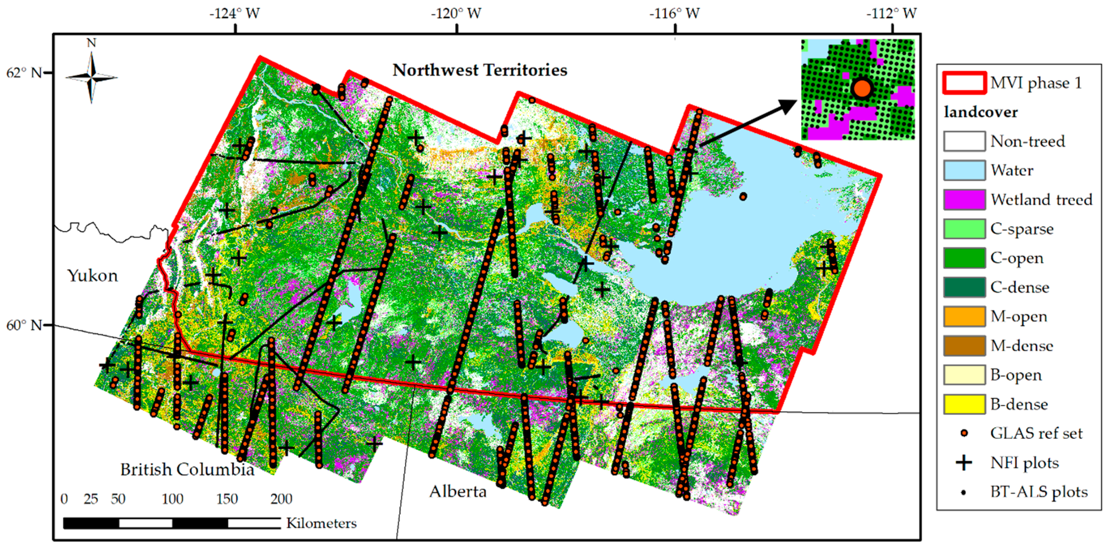
2.1. Study Area

For this paper, the mapping area (Figure 1, red outline), also known within the MVI project [5] as Phase 1, has 2007 as reference year and a 151,700 km² extent. Phase 1 is mostly located within the High and Mid-Boreal Ecoregions of the Taiga Plains Ecozone [40] (Figure 1), which contains the more productive forests of NWT. From the 1970s to 2010, only 24% of the study area was mapped by conventional forest inventory. According to a ca. 2007 Landsat-based landcover map (Section 2.2.3, Figure 1) detailed in Castilla et al. [5] that was used in this study to stratify the mapping area by forest cover types, about 65% of the study area is covered by forested lands largely dominated by upland conifer stands (open: 42% of the forested area, dense: 18%, sparse: 11%), upland mixedwood stands (dense: 10%, open: 1%) and coniferous wetland treed areas (12%), with a few areas dominated by upland broadleaf stands (dense: 4%, open: 2%) (Figure 2). The main needle leaf species are black spruce (Picea mariana (Mill.) Britton, Sterns and Poggenb.), jack pine (Pinus banksiana Lamb.), white spruce (Picea glauca (Moench) Voss) and tamarack (Larix laricina (Du Roi) K. Koch) whereas the dominant broadleaf species are trembling aspen (Populus tremuloides Michx.) and balsam poplar (Populus balsamifera L.). The topography is generally gently rolling except in a small western part of the area located within the Boreal Cordillera Ecozone that has high reliefs and steep slopes.

2.2. Datasets

Input datasets (upper row of Figure 3) required in our k-NN workflow to produce the ca. 2007 raster maps of forest attributes (also known within the MVI project [5] as the Satellite Vegetation Inventory, SVI) consist of: (i) point dataset of response variables (i.e., forest attributes to be mapped) modelled from GLAS, (ii) wall-to-wall datasets of feature variables from remote sensing and other sources, (iii) ancillary data, (iv) independent validation datasets, and (v) Landsat-based maps.

2.2.1. Response Variables

The following five forest attributes were used as response variables in the k-NN algorithm:

• Stand height (Ht, m): average height of dominant and codominant live trees, i.e., with height ≥ average Lorey’s height, where Lorey’s height is the average height of all trees with diameter at breast height (DBH) ≥5 cm and taller than 1.3 m) weighted by stem cross-section;
• Crown closure (CC, %): percent tree cover;
• Stand volume (Vs, m³·ha⁻¹): sum of volume inside bark of the boles of live trees with height ≥ Lorey’s height;
• Total volume (Vt, m³·ha⁻¹): sum of volume inside bark of the boles of all live trees with DBH ≥ 5 cm;
• Total aboveground biomass (AGB, t·ha⁻¹): total dry mass per unit area of whole live trees with DBH > 5 cm, including branches and leaves and excluding roots based on models reported in [41,42].

These forest attributes were estimated for the reference dataset of surrogate FI plots using ALS and GLAS LiDAR models as previously reported in [5,7] and as summarized in Methods (Section 2.3.1).

2.2.2. Feature Variables from Remote Sensing and Other Sources

On the basis of similar studies in Canada [7,8,16,43], we considered a number of feature variables with the following criteria: (i) known correlation to forest attributes, (ii) publicly available as wall-to-wall geospatial layers, (iii) native spatial resolution deemed sufficient (25–100 m) for mapping attributes with a 30 m pixel size, and (iv) for satellite imagery, orthorectified and calibrated radiometry with acquisition within plus or minus 1 year relative to the reference mapping year of 2007. By this standard, we gathered across the study area, satellite imagery from both Landsat 5 Thematic Mapper (TM) and ALOS-1/PALSAR, and environmental datasets, both biotic and abiotic, obtained from several sources (

Table 1. Description of categorized candidate feature variables for k-NN prediction and mapping. Labels with an * indicate feature variables selected as input to the k-NN mapping.

Feature Category	Description	Label	Units	Year	Pixel Size
Landsat TM spectral bands, indices and texture (LANDSAT)	Blue band TOA a reflectance	B1	-	2006–2008	30 m
	Green band TOA reflectance	B2	-
	Red band TOA reflectance	B3 *	-
	Near-infrared band TOA reflectance	B4 *	-
	Short-wave infrared band TOA reflectance	B5	-
	Short-wave infrared band TOA reflectance	B7 *	-
	Normalized Difference Vegetation Index (B4 − B3)/(B4 + B3)	NDVI	-
	Reduced Simple Ratio (B4/B3) ∗ (B5max − B5)/(B5range)	RSR *	-
	Normalized Difference Moisture Index (B4 − B5)/(B4 + B5)	NDMI	-
	Texture: 3 × 3 variance of near-infrared band	B4_TEX	-
PALSAR dual-polarized backscatter and texture (PALSAR)	HH-polarized L-band backscatter intensity	HH	-	2007	25 m
	HV-polarized L-band backscatter intensity	HV *	-
	HV/HH backscatter intensity ratio	HVHH	-
	Texture: HH 9 × 9 CV b	HH_ TEX	-
	Texture: HV 9 × 9 CV	HV_TEX	-
	Texture: HV/HH 9 × 9 CV	HVHH_TEX	-
Environmental c	2000 percent tree cover map updated to 2007	TC *	%	2007	30 m
	Terrain elevation from CDED d	ELEV *	m	variable	90 m
	Terrain slope from CDED	SLOPE *	deg	variable	90 m
	Compound Topographic Index from CDED	CTI	-	variable	90 m
	Average Soil Moisture Index	SMI *	mm	2001–2010	100 m
	Average Climatic Moisture Index	CMI	cm	2001–2010	100 m

^a Top-of-atmosphere. ^b Coefficient of variation. ^c Includes biotic and abiotic features. ^d Canadian digital elevation data.

).

For Landsat imagery, we downloaded (https://earthexplorer.usgs.gov/, accessed: 7 August 2009) 8 orthorectified 30 m resolution Landsat 5 TM scenes (183 km by 170 km) in level L1G at-sensor radiance format for spectral bands 1 to 5 and band 7 from years 2006 to 2008, each acquired within the growing season (mid-June to end of August). Scenes within ±1 year of the 2007 reference year had to be collected for some portions of the study area to generate the best possible cloud and haze-free imagery.

For PALSAR imagery, we downloaded 49 1° × 1° tiles for the year 2007 from the global 25 m resolution PALSAR mosaic (2007–2010)—version 1 (https://www.eorc.jaxa.jp/ALOS/en/dataset/fnf/fnf_palsar20140116_e.htm, accessed: 1 November 2015). These tiles provided orthorectified L-band dual-polarized SAR mosaics at 25 m pixels, namely 16 bit HH- and HV-polarized terrain-corrected backscatter (gamma-naught) amplitude [44].

As an environmental biotic feature, we used the global percent tree cover product (TC) for the year 2000 at 30 m pixel size derived from Landsat data [45]. For abiotic environmental features, topography was characterized using the Canadian Digital Elevation Data (CDED) [46] at 90 m pixels. Finally, we considered 2 climatic features: the climate moisture index (CMI) [47] and the soil moisture index (SMI) [48] at 100 m pixels. Topographic and climatic features are commonly used to improve wall-to-wall forest attribute estimation [26,49]. Processing of all above datasets, required prior to their usage in k-NN mapping, is described in Methods (Section 2.3.2).

2.2.3. Ancillary Data

We used the ca. 2007 Landsat-based landcover map at 30 m pixels produced by the MVI project (see details in [5,50]). The study area includes 8 out of 10 possible forest classes combining 3 forest cover types (conifer, mixedwood and broadleaf) with 3 density classes (sparse, open, dense), plus a wetland treed class (map in Figure 1, histogram of forest classes in Figure 2). This landcover map was used to define target forest pixels for k-NN predictions and mapping and assess prediction accuracy across forest types.

We also used the Landsat-based yearly tree cover loss product (2000–2015) with 30 m pixels [45] (http://earthenginepartners.appspot.com/science-2013-global-forest, accessed: 8 september 2015) that we filtered to remove isolated change pixels using a 3 × 3 sieve filter. Yearly tree cover losses accounted for forest changes (harvest, fire) between the various acquisition years of all datasets encompassing the period 2000–2010.

2.2.4. Independent Validation Datasets

Two sample sets were used as independent validation datasets:

• Fifty-two 400 m² NFI ground plots [51,52] (hereafter NFI plots) for which stand-level forest attributes derived from a combination of ground measurements and allometric equations were available as continuous variables, except for crown closure provided in broad ordinal classes. NFI plots qualify as an independent validation set as they provide a probabilistic sample set but with the caveat that it is a relatively small sample size for the study area;
• Over 1 million Boreal transect ALS 25 m cells (hereafter BT−ALS LiDAR plots) derived from ALS data acquired in the summer of 2010 along 750 m wide transects totalling 1800 km in length with a point sampling density of 2.8 point·m⁻² [53,54]. Stand height, Lorey’s height, and crown closure were estimated from ALS models, while stand volume was estimated from stand height, and both total volume and AGB were estimated from average Lorey’s height [5]. However, crown closure estimates were not retained for validation because of a laser power issue preventing the proper transferability of the ALS-based crown closure model to the BT−ALS data [7]. Although the BT−ALS sample set does not provide attribute estimates as accurate as those from the NFI ground plots, and thus qualifies more as a comparison rather than a validation set, we still considered it to be a valuable independent validation dataset. It has a large number of 25 m cells and its extensive spatial extent captures a much wider geographic range of forest conditions across broad forest types than NFI ground plots.

2.2.5. Landsat-Based Forest Attribute Maps

We used two previously published 30 m Landsat-based maps of stand height and AGB, respectively:

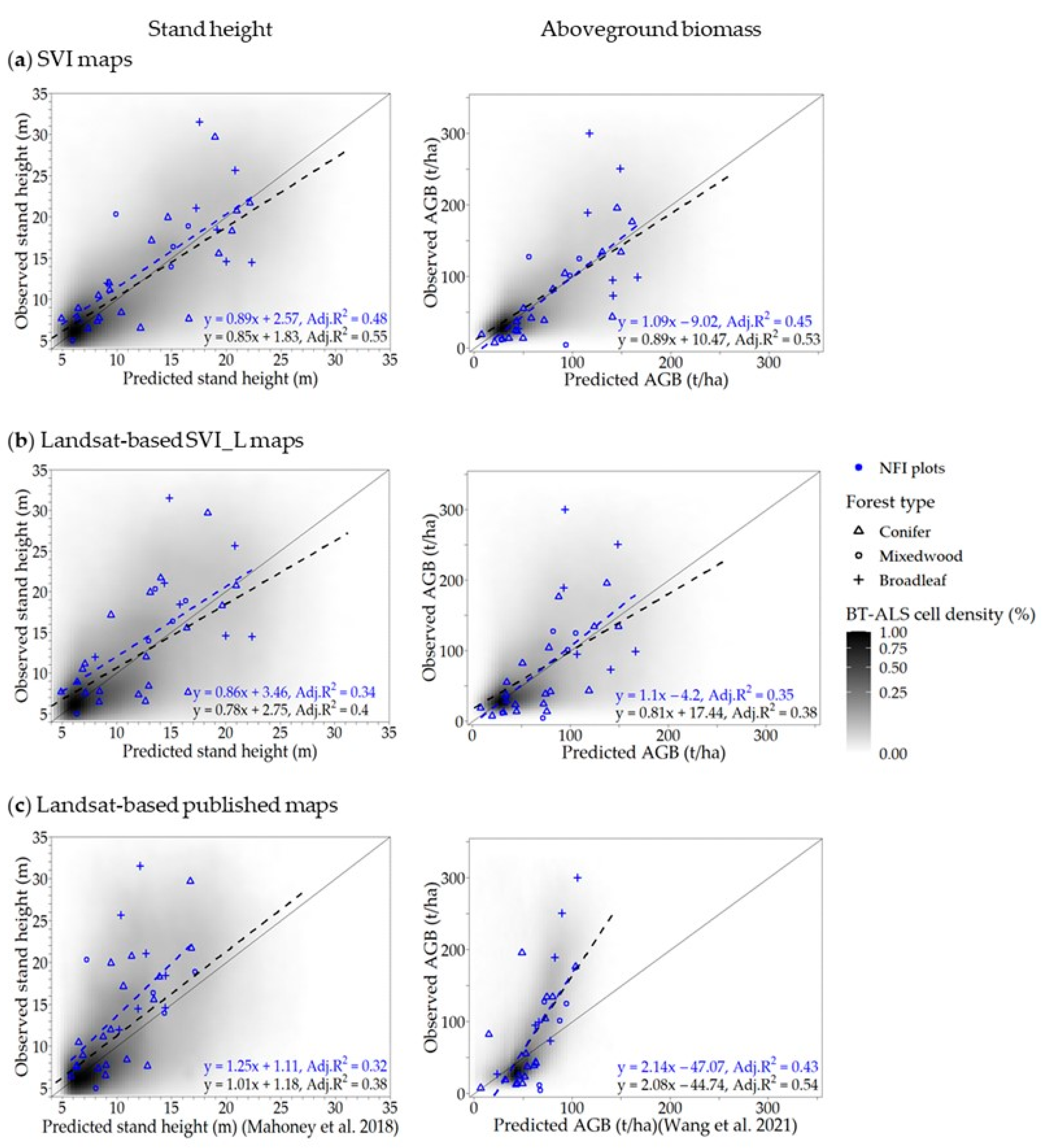
• The ca. 2007 k-NN map of stand height over the same extent from Mahoney et al. [7];
• The large-area 2007 AGB map of Wang et al. [55] covering northwestern Canada and Alaska; this map was part of a 1984–2014 time series of 30 m annual AGB maps derived from the Gradient Boosted Machines machine learning algorithm trained by GLAS-based AGB estimates and using predictors from seasonally fit Landsat time series.

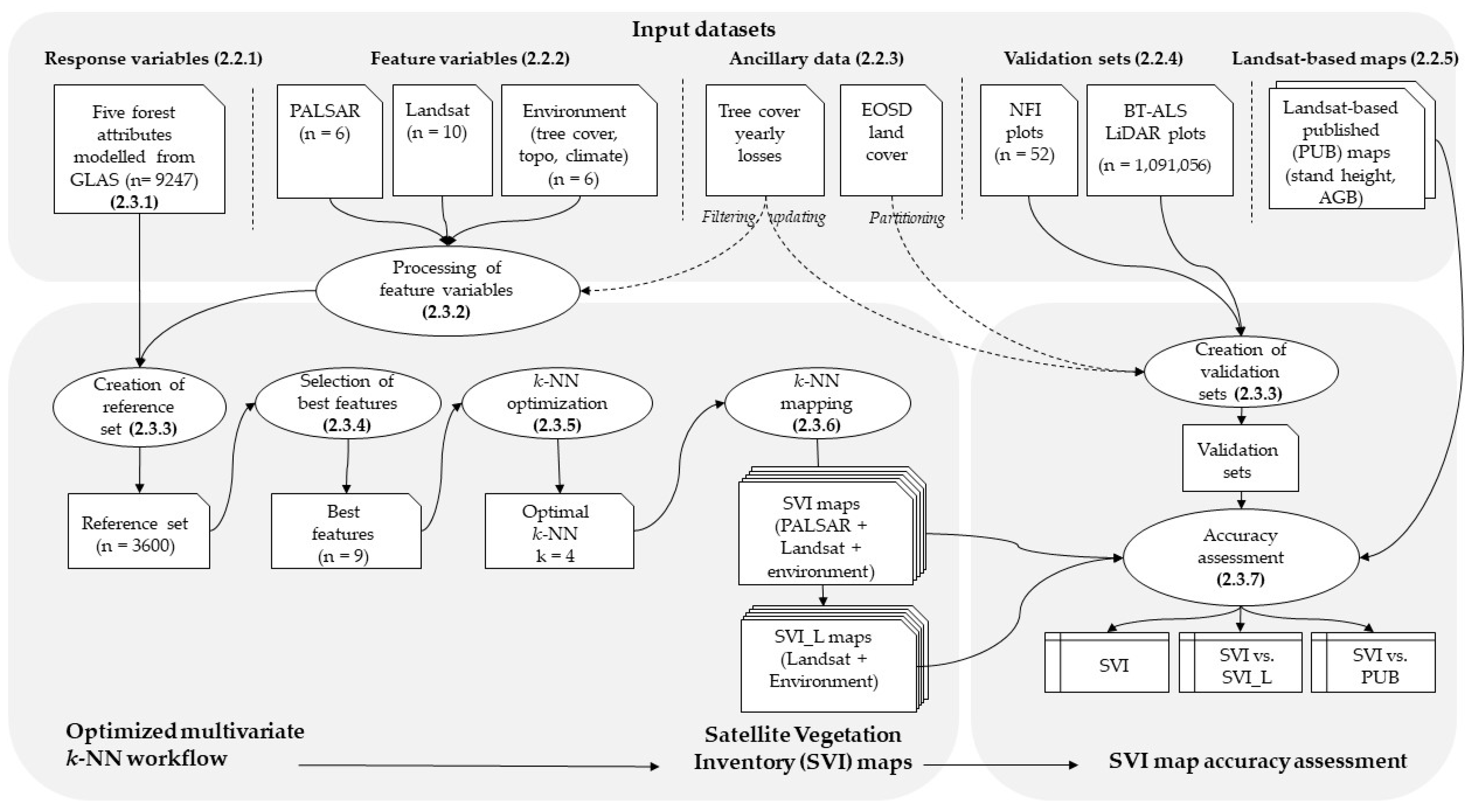
We selected these two maps as they were also produced using machine learning algorithms that were trained using GLAS-modelled attributes and a feature dataset that employed similar yet different environmental and Landsat features. In addition, we created a version of our maps of stand height and AGB that excluded PALSAR from the feature dataset (a version we call SVI_L, L for Landsat, see Section 2.3.6). These two sets of Landsat-based stand height and AGB maps, created without any PALSAR features, were used as baseline maps to quantify accuracy gains brought by the integration of PALSAR features.

2.3. Methods

The k-NN algorithm finds, for each forested target pixel with unknown forest attributes (response variables), the k most similar reference pixels to the target pixel and predicts the value of the forest attributes as a combination of the values in those reference pixels [27]. Similarity is measured in the multidimensional space of the auxiliary feature variables using various distance metrics, common ones being Euclidian, Mahalanobis, and most similar neighbour (MSN) [26]. For each target forested pixel, the values of the five forest attributes are predicted as the average of the k reference pixels (i.e., the pixels corresponding to the centroids of the GLAS footprints used as surrogate FI plots) that are nearest to the target pixel in the space of feature variables as follows [27]:

$${\tilde{y}}_i=\frac{{{\displaystyle \sum }}_{j=1}^k{w}_j^i{y}_j^i}{{{\displaystyle \sum }}_{j=1}^k{w}_j^i}, w_j^i=\frac{1}{D_{ij}^{t_d}}$$

(1)

where ${\tilde{y}}_i$ is the predicted attribute for the ith target pixel, $\left\{y_j^i;j=1, \dots , k\right\}$ is the set of observed response variables for the jth reference GLAS surrogate FI plots nearest in the feature space to the ith target pixel, weights $w_j^i$ are given by the inverse of the distance $D_{ij}^{}$ in the feature space on the basis of a given distance metric between the ith target pixel and the jth nearest reference pixel, and exponent $t_d$ usually takes on values $t_d$= 0 (simple average) or 1 (inverse distance weighted average).

Our k-NN workflow (Figure 3), adapted from Beaudoin et al. [43], includes the following pre-processing steps of input datasets: (i) GLAS modelling of response variables, (ii) processing of feature variables, and (iii) creation of a reference set of GLAS surrogate FI plots along with two independent validation sets. Then the steps specific to k-NN mapping and accuracy assessment includes (iv) selection of the best feature variables among those from the Landsat, PALSAR, and environmental datasets, (v) optimization of k-NN parameters, (vi) creation of forest attribute SVI raster maps from k-NN predictions, and (vii) accuracy assessment of SVI maps including a comparative evaluation with a Landsat-based SVI map version and with previously published Landsat-based maps.

2.3.1. GLAS Modelling of Response Variables

The values of the 5 forest attributes (Section 2.2.1) in the reference dataset were estimated using 2-stage predictive models based on (i) 38 field plots with ALS data for the 1st stage models and (ii) 43 GLAS footprints that had coincident ALS data for the 2nd stage models (see [5,7] for more information). Lorey’s height (i.e., weighted mean height of trees, with weight proportional to the area of the trunk cross-section), stand height, and crown closure was modelled from 2 distinct GLAS metrics (

Table 2. Geoscience Laser Altimeter System (GLAS) models of forest attributes along with model form and coefficients, goodness of fit (adj. R²) and root mean square error (RMSE) values (adapted from Tables 3 and 4a in [5]).

Forest Attribute	Model and Parameters	Adj. R2	RMSE
Lorey’s height (HL, m) a	HLGLAS = 2.46 + 0.91 × P85 b	0.89	1.1
Stand height (Ht, m)	HtGLAS = 2.30 + 1.10 × P85	0.88	1.3
Crown closure (CC, %)	CCGLAS = 64.63 × Lz0.25 c	0.54	6.5
Stand volume (Vs, m3·ha−1)	VsGLAS = 0.61 × HtGLAS1.84	0.76	46.8
Total volume (Vt, m3·ha−1)	VtGLAS = 1.84 × HLGLAS1.69	0.81	59.3
Aboveground biomass (AGB, t·ha−1)	AGBGLAS = 2.27 × HLGLAS1.45	0.76	35.7

^a Intermediate modelled attribute not targeted for k-NN mapping. ^b P85: GLAS waveform 85th percentile. ^c Lz: cumulative projected foliage area index.

). Stand volume, total volume, and AGB were modelled from the GLAS estimates of stand height and Lorey’s height, respectively (Table 2). The GLAS models were subsequently applied to all GLAS footprints in the study area, thereby creating GLAS surrogate FI plots.

2.3.2. Processing of Feature Variables

The spectral bands 1 to 5 and band 7 of the 2006–2008 summer TM images were normalized to a MODIS Top-of-Atmosphere (TOA) reflectance 250 m monthly composite [56] to balance the radiometry across all images, providing a mostly seamless ca. 2007 Landsat TM TOA reflectance mosaic (Table 1). In addition, we derived three commonly used spectral indices, namely the normalized difference vegetation index (NDVI), its variant the Reduced Simple Ratio (RSR) [57] and the normalized difference moisture index (NDMI). Finally, we added as texture feature the variance in band 4 over a 3 × 3 moving window (B4_TEX) for a total of 10 Landsat features (Table 1).

For the PALSAR features, the contiguous 2007 HV and HH gamma-naught backscatter amplitude tiles were mosaicked and clipped to the extent of the Landsat mosaic. The backscatter amplitude pixel values were squared into intensity values and filtered for speckle noise using the Touzi multi-resolution speckle filter with an 11 × 11 window [58]. Next, we derived the cross-polarized ratio HV/HH (HVHH). Finally, the local coefficient of variation was calculated over a 9 × 9 moving window for each of the 3 unfiltered mosaics providing first-order texture features (HH_TEX, HV_TEX, HVHH_TEX) [38]. This processing provided a total of six PALSAR features (Table 1).

For the environmental biotic feature, the global 2000 percent tree cover product (TC) was updated to year 2007, using yearly tree cover loss [45] as in Beaudoin et al. [6]. For the environmental abiotic features, the CDED provided terrain elevation (ELEV) with 90 m pixel from which we derived local slope (SLOPE) and compound topographic index (CTI) [59]. The two climatic features, CMI and SMI, were used as provided for a total of six environmental features (Table 1).

All of the above datasets, provided in various file formats, ground resolutions (Table 1), and projections, were re-projected to Albers equal area conic projection with a 30 m pixel size using bilinear interpolation, were clipped to the extent of the study area and were saved as a stack of geoTIFF files.

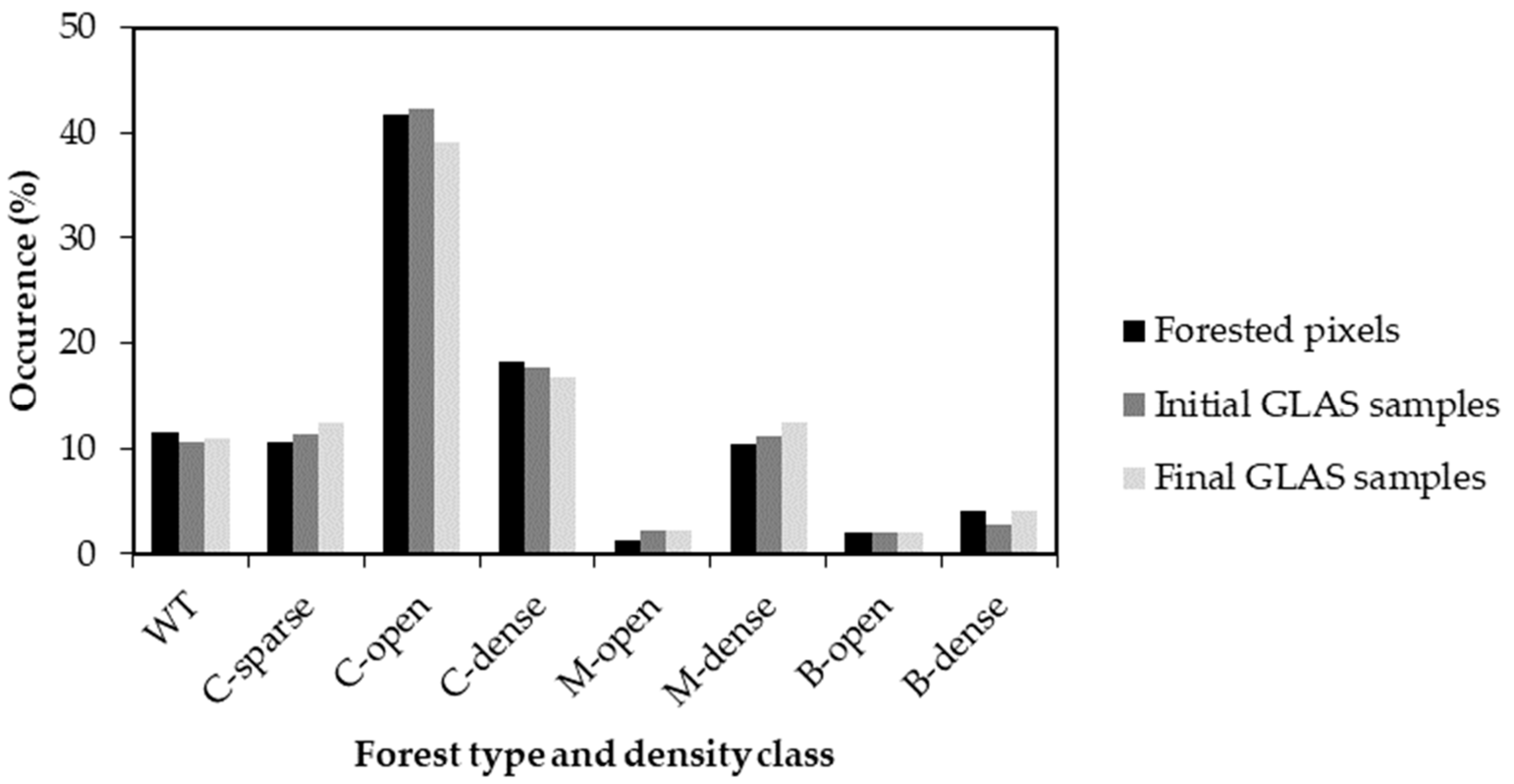
2.3.3. Creation of Reference and Validation Datasets

To create the reference dataset of GLAS-based surrogate FI plots, we screened all available GLAS 2A and 3A footprints in the study area to discard footprints potentially affected by noise from the atmosphere, topography (slope > 5°), or snow cover [7]. This resulted in an initial selection of 9247 surrogate FI plots. Next, we applied an additional screening by using the yearly cover loss maps to exclude GLAS footprints that were disturbed before or during the 2006–2008 years of Landsat and PALSAR acquisitions. Furthermore, to reduce the effect of spatial autocorrelation, we selected a smaller subset in which no 2 footprints were closer to each other than 500 m. The latter was the autocorrelation range found by a semi-variogram analysis [6]. A downside of this approach was a reduction in the range of reference attribute values, which in turn increases k-NN prediction bias [39]. Therefore, excluded initial footprints that were below the 1% or above the 99% percentiles were reintroduced.

The filtering process generated a final reference set of 3600 out of 9247 GLAS surrogate FI plots that were well distributed across the study area (Figure 1). Histograms of forest landcover classes for the final selection of GLAS samples of surrogate FI plots were similar to the initial GLAS samples and of all forested pixels within the study area (Figure 2). Noticeably, Pearson correlation coefficient r among the 5 attributes showed that stand volume and total volume were highly correlated to AGB in the reference dataset (r > 0.95, p < 0.001) (Table S1). Such high correlation arises from the fact that AGB and total volume were both derived from GLAS-based estimates of Lorey’s height, whereas total volume was derived from GLAS-based estimates of stand height (Table 2), itself highly correlated to Lorey’s height.

For the validation datasets, we discarded NFI and BT−ALS LiDAR plots that were either (i) non-forested or wetland treed according to the landcover map, (ii) located over sloping terrain (slope > 5 degrees), and (iii) disturbed between their measurement year and the 2006–2008 years of Landsat and PALSAR acquisitions according to the yearly tree cover loss map. This process resulted in selecting (i) 31 NFI plots out of 53 in the study area (19 conifer, 7 mixedwood, and 5 broadleaf samples), and (ii) 1,080,866 BT−ALS LiDAR plots (76.9% conifer, 13.6% mixedwood, and 9.5% broadleaf samples) (

Table 3. Descriptive statistics for ‘’observed’’ stand height and aboveground biomass (AGB) using all samples that are also partitioned by three forest cover types for (a) reference set from GLAS surrogate and (b) two validation sets: National Forest Inventory (NFI) plots and BT−ALS LiDAR plots. Descriptive statistics for all five attributes are reported in Table S2.

			(a) Reference Set				(b) Validation Sets
			GLAS				NFI a					BT−ALS
Attribute	Forest Type	n	Min	Max	Mean	SD b	n	Min	Max	Mean	SD	n	Min	Max	Mean	SD
Stand height (m)	ALL	3600	3.6	34.1	9.7	5.9	31	5.0	31.5	14.8	7.0	1,080,866	2.5	35.0	11.6	6.1
	Conifer	2459	3.6	33.6	8.8	4.8	19	6.5	29.7	12.9	6.6	831,619	2.5	34.8	10.0	5.0
	Mixedwood	528	3.7	34.1	13.5	7.4	7	12.0	31.5	19.7	7.0	146,738	2.6	34.9	16.5	6.7
	Broadleaf	219	3.7	34.0	15.7	8.3	5	5.0	20.4	14.9	6.1	102,509	2.6	35.0	17.4	6.1
AGB (t·ha−1)	ALL	3600	1.2	352.1	54.2	51.6	30	4.5	300.1	85.4	77.0	1,080,734	7.9	326.4	72.1	55.1
	Conifer	2459	15.1	286.5	49.2	38.6	18	7.6	195.8	64.4	59.6	831,499	7.9	324.4	57.9	43.5
	Mixedwood	528	15.9	292.6	87.2	64.8	7	26.7	300.1	147.7	100.8	146,726	8.2	325.9	116.3	64.3
	Broadleaf	219	15.9	290.6	107.0	73.1	5	4.5	127.5	74.0	61.2	102,509	8.3	326.4	124.3	59.8

^a samples with numbers in black italic font not used for validation due to small sample size. ^b standard deviation.

b). Due to data gaps, a slightly smaller validation sample was produced for the accuracy assessment of Wang’s AGB map (Table 3b).

Descriptive statistics of the GLAS reference set and two validation datasets for stand height and AGB are shown in Table 3 (see Table S2 for all five attributes). The GLAS-modelled forest attributes in the reference dataset (all forest cover types combined) were relatively similar to those of conifers, which dominate the study area (Table 3a). The distribution was skewed towards sparse and open conifer stands with smaller attribute values compared with the taller and more stocked broadleaf and mixedwood forest types. Average stand height was the smallest for conifers, with larger values for broadleaf and mixedwood forest types, a result that was consistent in both the reference and validation datasets (Table 3a,b). Average AGB were largest and most variable for broadleaf stands, followed by mixedwood stands, and smallest for conifer stands, a result that was consistent for both the GLAS reference and validation datasets (Table 3).

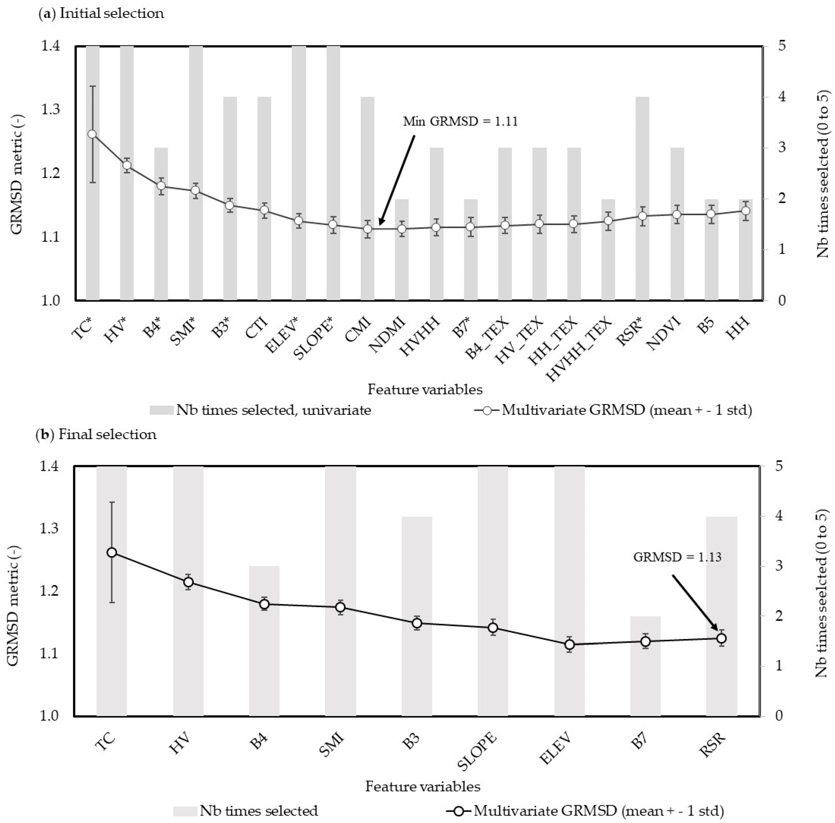
2.3.4. Selection of Best Feature Variables

The purpose of this procedure was to avoid ingesting noisy or highly correlated feature variables into the k-NN process [27]. Initially, this was done by visual inspection of the feature variables. In particular, bands 1 and 2 of the ca. 2007 Landsat TM TOA reflectance mosaic were removed due to residual atmospheric artifacts. Among those that passed the visual inspection, we selected the best feature subset using the varSelection procedure within the yaImpute R package [60] using the forward selection mode “addVars” and the MSN distance metric as in Beaudoin et al. [43]. The varSelection procedure uses the global root mean square difference (GRMSD) as a single multivariate accuracy metric that was calculated between observed and predicted forest attribute values projected in the Mahalanobis space using n = 30 bootstrap samples [60]. An iterative forward selection procedure finds the single best feature that yields the lowest GRMSD, with successive features being sequentially added by decreasing GRMSD values until these values reach a minimal value as a saddle point. Beyond this saddle point, GRMSD values increase due to the addition of noisy features that are less correlated to the response variables.

The feature selection procedure was applied first in univariate mode to assess each feature for its predictive capacity separately for each of the five individual forest attributes and to record the number of times it was selected across the five attributes. Multivariate mode was subsequently used to assess the overall predictive capacity of the best features selected at once for all five forest attributes. We assessed the best feature selection by reapplying the iterative forward selection procedure described above to ensure low GRMSD levels without any substantial increase for the last selected features.

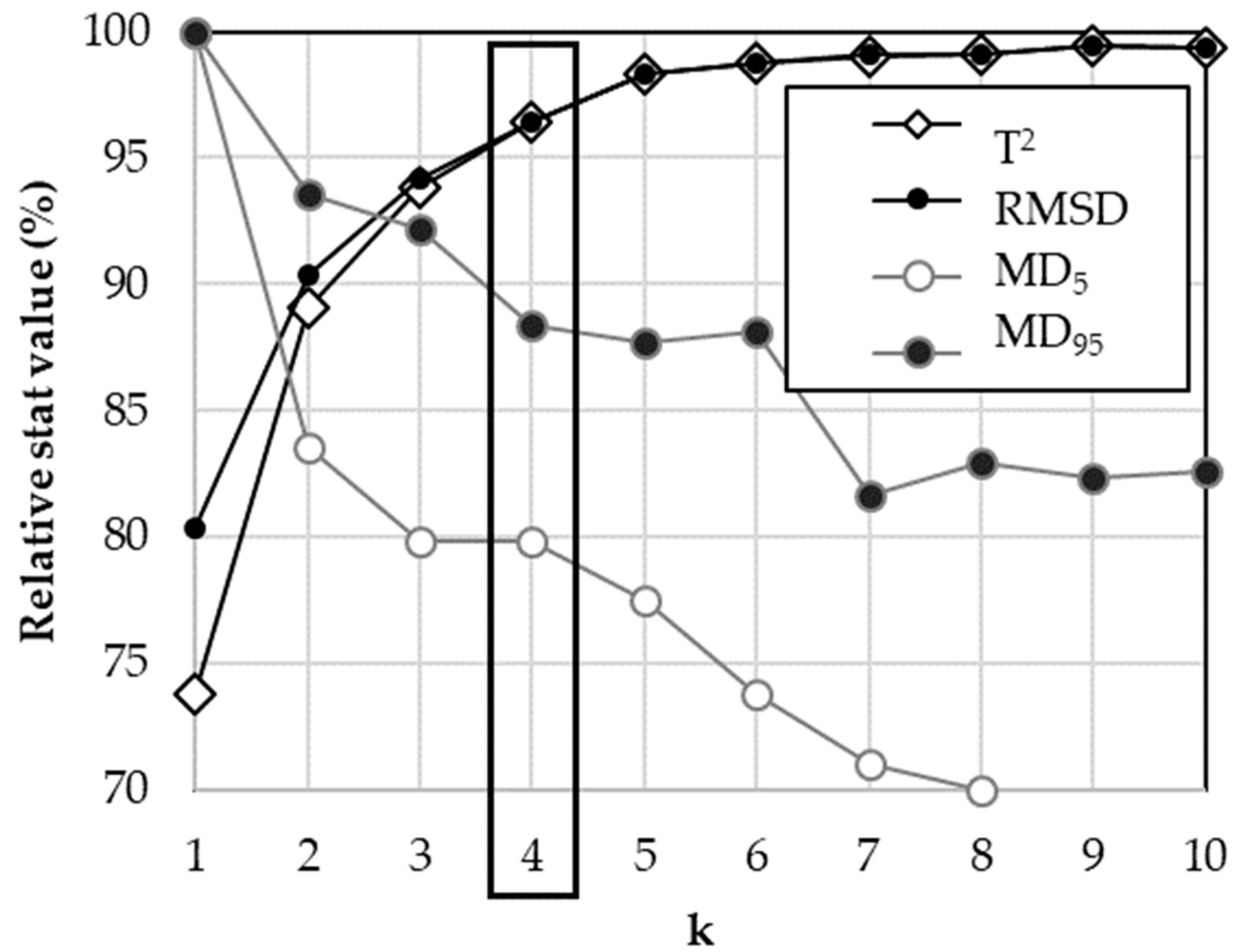
2.3.5. Optimization of k-NN k Parameters

In this paper, we used the Euclidian distance metric with simple averaging (t_d = 0 in Equation (1)). The optimization of the k value was determined using a five-fold cross-validation analysis undertaken on the reference dataset based on k-NN predictions using the yaImpute R package [61]. For a given value of k, ranging from 1 to 15, we computed for each of 5 forest attributes the following 5 statistics: T² (pseudo-R², [27], Equation (2)), as a measure of goodness of fit; root mean square difference (RMSD, [61], Equation (3)), indicative of overall accuracy; mean difference (MD, Equation (4)), indicative of bias; and MD for surrogate FI plots within the 5% lower tail (MD₅, Equation (5)) and upper tail (MD₉₅, Equation (6)) which indicate the over- and underestimation biases found at the lower and upper distribution tails, respectively [43].

$$T^2=\frac{\left({\mathrm{SS}}_{\mathrm{mean}}-{\mathrm{SS}}_{\mathrm{err}}\right)}{{\mathrm{SS}}_{\mathrm{mean}}}$$

(2)

$$RMSD=\sqrt{\frac{1}{n}{{\displaystyle \sum }}_{i=1}^n{\left({\tilde{y}}_i-y_i\right)}^2}$$

(3)

$$MD=\frac{1}{n}{{\displaystyle \sum }}_{i=1}^n\left({\tilde{y}}_i-y_i\right)$$

(4)

$$M{D}_5=\frac{1}{l}{{\displaystyle \sum }}_{i=1}^l\left({\tilde{y}}_i-y_i\right)|y_i<y\left(rank\left(y,0.05n\right)\right)$$

(5)

$$M{D}_{95}=\frac{1}{u}{{\displaystyle \sum }}_{i=1}^u\left({\tilde{y}}_i-y_i\right)|y_i>y\left(rank\left(y,0.95n\right)\right)$$

(6)

where SS_mean and SS_err are the squared sum of differences between the observations and the mean and between the observations and the predictions, respectively, n is the number of GLAS surrogate FI plots, ${\tilde{y}}_i$ and y_i are the predicted and observed attribute values in surrogate FI plot, respectively, l and u are the number of surrogate FI plots in the lower and upper tails of the distribution of forest attribute y, respectively, and y(rank(y, P∙n)) is the value corresponding to the P percentile of attribute y.

For each forest attribute, the 5 statistics described in equations 2 to 6 were calculated using a 20% random sample cross-validation fold that was repeated 5 times, from which a mean value was obtained for each statistic. To compare the statistics among attributes, we normalized the statistics relative to the mean observed attribute value (percent value). Each of the five normalized statistics was further averaged across the five attributes to compute a single “multivariate” value per statistic [43]. Finally, each of the five multivariate statistics was converted into a percent value relative to its optimal value (rel_{stat_opt}) found across the range of k values. The optimal value is the maximum value for T² and the minimum value for the four other statistics adapted from [27].

Graphs of rel_{stat_opt} versus k values were used to select the best k value as a compromise between (i) the reduction of overestimation at low values and underestimation at high values of the forest attributes, which requires lower k values and (ii) the reduction of prediction variance and augmentation of the goodness of fit, which requires higher k values [39].

2.3.6. Forest Attribute Maps from k-NN

The SVI raster maps of the five forest attributes were produced as a stack of GeoTIFF files from an in-house C++ k-NN routine (k-NNMapping, [43]) that provides very fast and exact k-NN predictions using the Approximate Nearest Neighbour library [62]. Based on the landcover map, all 30 m forested pixels were assigned k-NN predictions for the 5 attributes, whereas non-forested pixels were assigned to no data. The k-NN predictions were obtained using the full set of best feature variables (Section 2.3.4) and the optimized k-NN k parameter value (Section 2.3.5).

In addition to the SVI maps derived from PALSAR, Landsat, and environmental features, we also created a Landsat-based SVI map version combining only Landsat and environmental features (hereafter SVI_L, L for Landsat).

2.3.7. Accuracy Assessment

The accuracy of the SVI maps (Section 2.3.6) and the two sets of Landsat-based maps (Section 2.2.5 and Section 2.3.6) was assessed separately using two independent validation datasets (NFI plots and BT−ALS LiDAR plots, Section 2.2.4). The accuracy metrics for the SVI maps were then compared to those from Landsat-based maps to assess the accuracy gains brought by our improved k-NN workflow including PALSAR features. The following accuracy metrics were obtained for each of the maps:

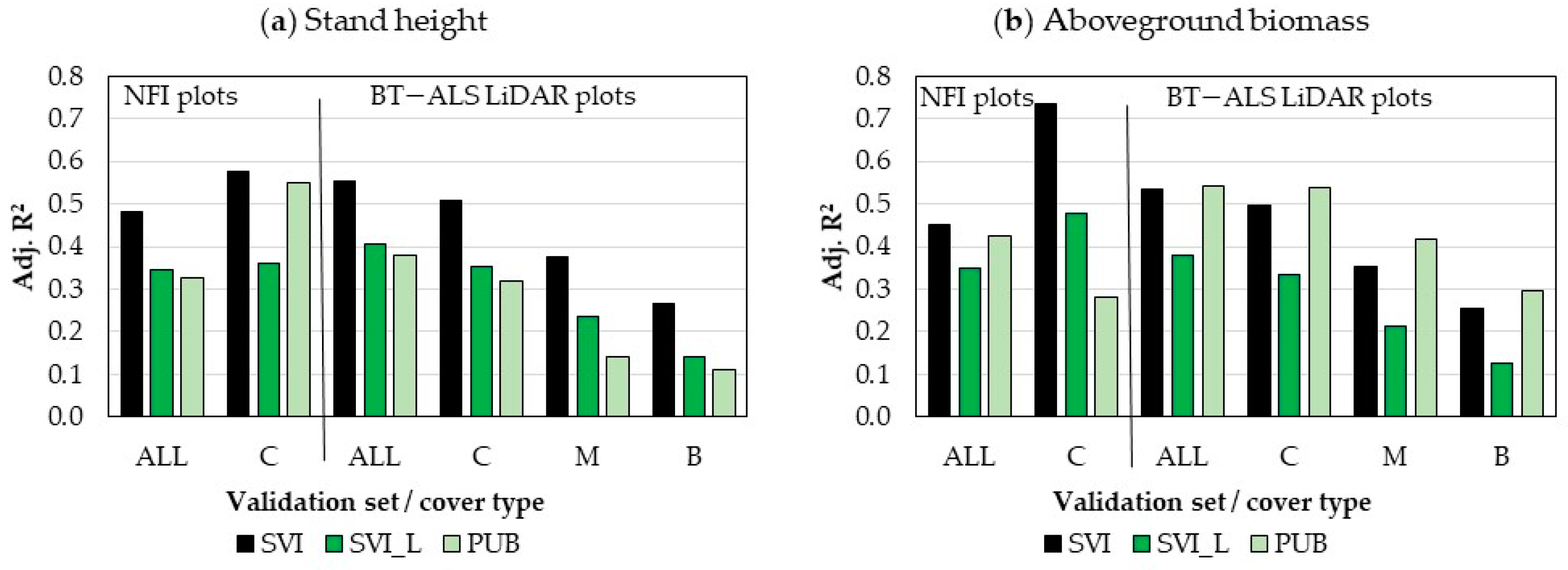
• goodness of fit (adj. R²) and coefficients of linear regressions (predictions ~ observations);
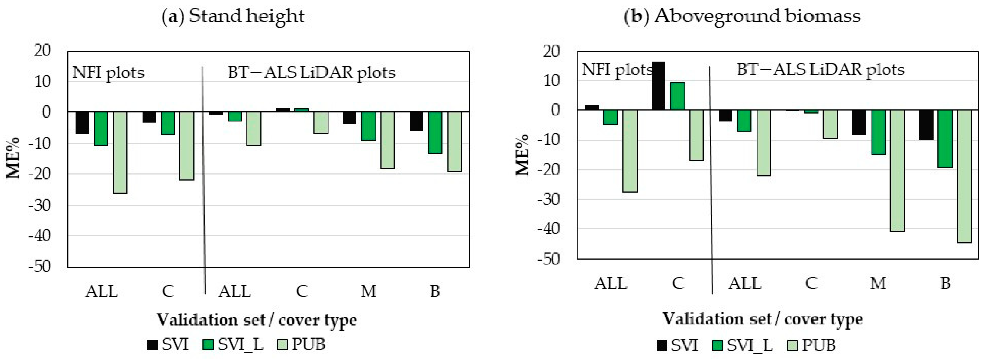
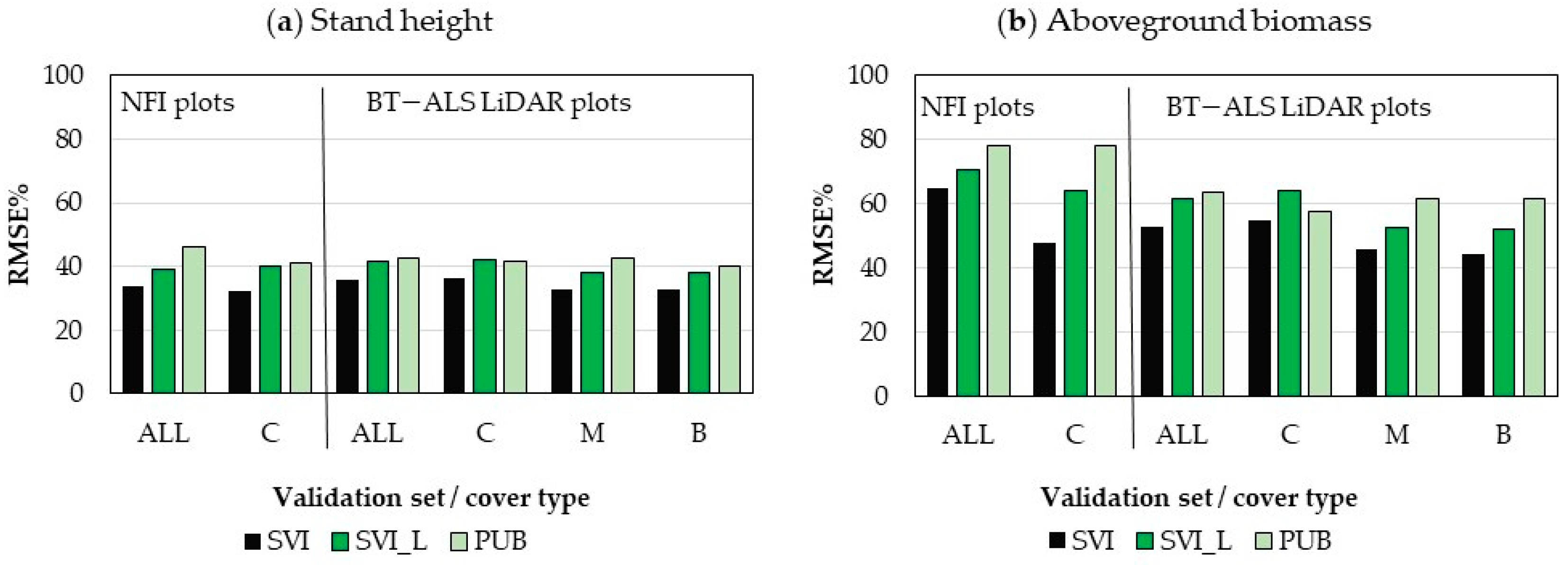
• mean error or bias (ME, predicted minus observed, expressed as in Equation (4) for MD) and root mean square error (RMSE, expressed as in Equation (3) for RMSD) as a measure of overall accuracy, both expressed as percent values relative to the observed mean value (ME%, RMSE%);
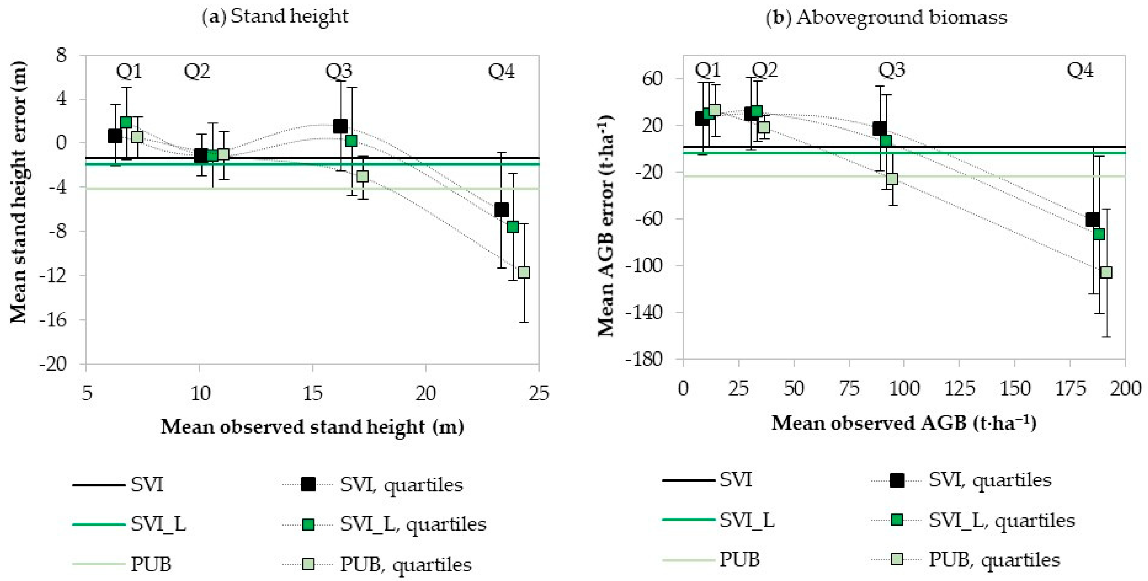
• mean and standard deviation of prediction error (predicted minus observed) by quartile group across the range of observed NFI attribute values. This is presented along with overall mean prediction error in a plot similar to a Bland Altman diagram [63,64], which provides a visual graphic of the magnitude and distribution of prediction bias and variance across the range of the response variable.

To assess the potential impact of forest type on accuracy, these metrics were computed first using all samples and then using samples partitioned by forest cover type for each of the two validation datasets.

Strictly speaking, the above accuracy metrics qualify as prediction errors only for the NFI plots, which come from a probability-based design and which have attribute values closer to the truth than the modelled attributes from the BT−ALS plots, but with the caveat of a small sample size. On the other hand, the BT−ALS plots provide a much larger sample set across all forest cover types, but being modelled, must be interpreted with caution.

3. Results

3.1. Selection of Best Feature Variables

Figure 4a shows the multivariate GRMSD curve as a function of the 20 feature variables selected in decreasing order of importance along with the number of times (0 up to 5) each feature was selected in univariate mode. GRMSD reached a minimal value of 1.11 with the selection of 9 features (up to the CMI climatic variable in Figure 4a). The overall best feature was the percent tree cover TC, which was systematically selected in univariate mode for all of the forest attributes but only once as best feature for crown closure (Figure S1). The second-best feature was the HV-polarized PALSAR backscatter, which was also systematically selected in univariate mode and, notably, was selected as best feature for all five attributes except for crown closure (Figure S1). The Landsat TM NIR (B4) and red (B3) bands were also selected among the best features, as well as three topographic features (CTI, ELEV and SLOPE) and two climatic features (CMI, SMI).

We refined the selection of best features based on the following adjustments. The Landsat-based RSR vegetation index, which was highly correlated with forest attributes (0.57 < r < 0.62), was not selected during the multivariate selection. As a result, it was readmitted to the set of best features. RSR was selected four out of five times in the univariate selection mode (Figure 4a). This suggests that the predictive power of RSR is somehow masked out during the multivariate selection process, and in this case is preferable to follow the outcome of the univariate selection. In addition, further visual inspection of the CTI variable revealed some artifacts over flat terrain, hence it was discarded. We also rejected the CMI variable because it was highly correlated with SMI (r = 0.96). Finally, we readmitted the Landsat SWIR (B7) band because it was a relatively good predictor for 2 attributes in the univariate selection mode (–0.59 < r < –0.47). We further validated this updated selection of 9 best features (highlighted by the ‘*’ symbol in Figure 4a and Table 1) by reapplying the VarSelection procedure in both multivariate and univariate modes. The resulting GRMSD curve (Figure 4b) shows a predictive response similar to that of the GRMSD curve using the initial selection of 9 features (Figure 4a), which attained a low GRMSD value of around 1.13, comparable to the value achieved in Figure 4a. Although the inclusion of B7 and RSR resulted in only a marginal increase in GRMSD, it was justified because both features were useful predictors for a number of attributes (Figure S1).

3.2. Optimization of the k-NN k Parameter

A value of k = 4 was selected from our multivariate optimization scheme based on 4 of the 5 relative statistics rel_{stat_opt} (%) across k values derived from Equations (2), (3), (5), and (6) (T², RMSD, MD₉₅, MD₅) (Figure 5). This decision considered the reduction of over- and underestimation biases (smallest MD₅ and MD₉₅) requiring the lowest possible k value while factoring the reduction in variance (smallest RMSD) and increase in goodness of fit (highest T²), both requiring larger k values (Figure 5). The k value of 4 allowed all relative statistics rel_{stat_opt} to be within 20% of their optimal values (100%) while keeping RMSD and T² values within 5% of their optimal values. This trade-off was selected to favour the reduction of variance to avoid grainy maps resulting from lower k values.

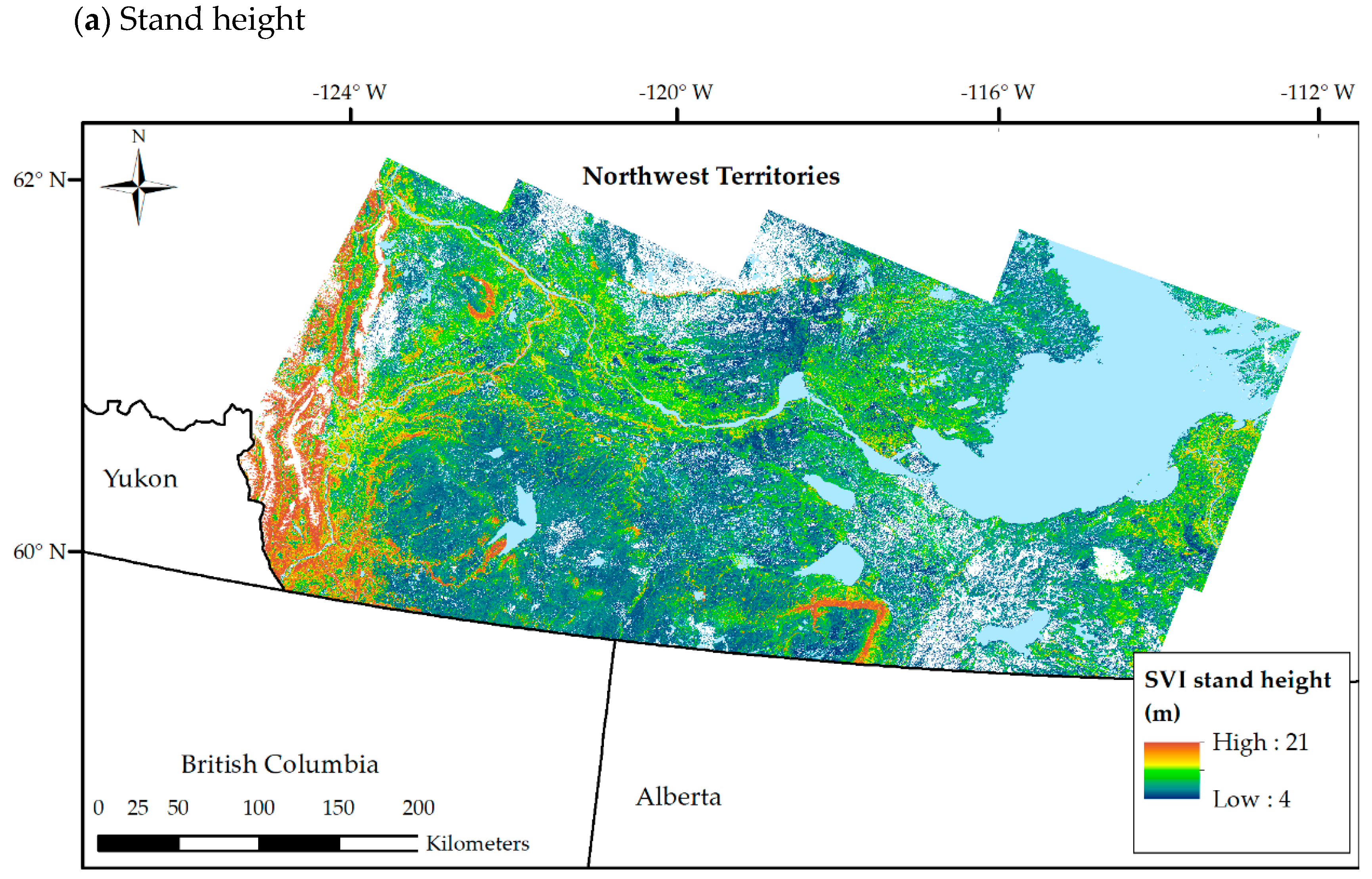
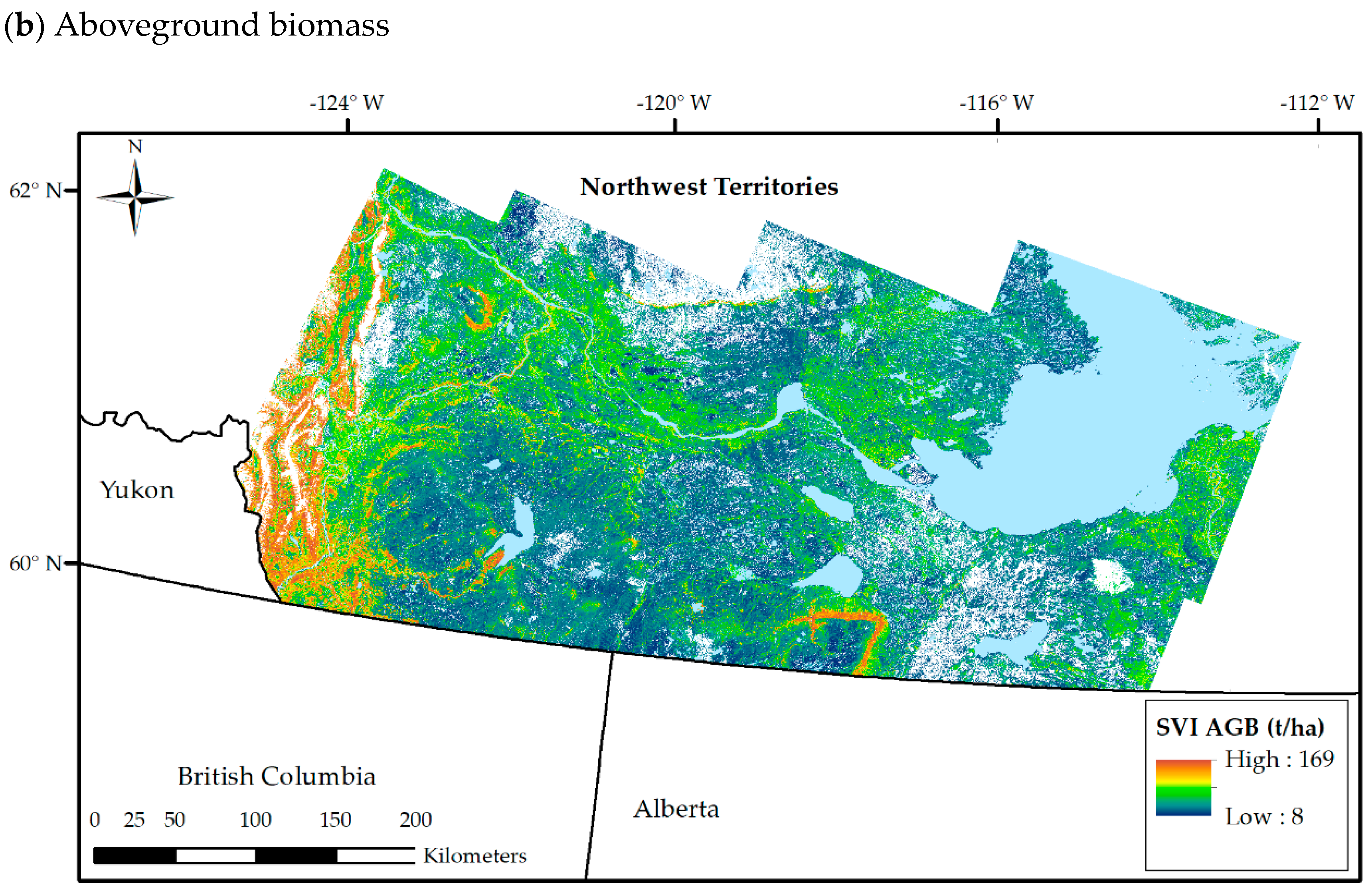
3.3. SVI Maps from k-NN

SVI maps of all five attributes were created from optimized multivariate k-NN predictions. Out of the five attributes, our focus is on stand height and AGB. This is because (i) the GLAS-based stand volume and total volume estimates in the reference dataset were highly correlated to AGB (r > 0.95, p < 0.001), resulting in similar SVI map patterns of stand and total volume to those of the SVI map of AGB and similar trends in accuracy metrics, (ii) the quality of SVI map of crown closure could not be properly evaluated as it is only reported by broad classes in the NFI plots and (iii) published Landsat-based maps used for comparison were only available for stand height and AGB. Maps and accuracy metrics for all SVI forest attributes (except crown closure, for the above reason) are available in the Supplementary Materials (Figure S2, Tables S3 and S4).

SVI maps of stand height and AGB are illustrated in Figure 6. The patterns matched well with the expectations for both high and low productivity areas, where higher productive forest regions in the west were consistent with the expected occurrence of forest stands with the largest stand height and AGB. Based on the analysis by Castilla et al. [5], they also reported the mapped SVI predictions were considered reasonable for conifer stands, which occupy over 70% of the forested area within the study area, and were relatively poorer for mixedwood and broadleaf stands.

3.4. Accuracy Assessment

3.4.1. Accuracy of SVI Maps

Pixel-level scatterplots of observed (NFI plots and BT−ALS LiDAR plots) versus predicted (SVI) values of stand height and AGB exhibited a similar pattern regardless of the validation dataset (Figure 7a). The linear regressions followed trends that approximated the 1:1 line, with similar slopes and intercepts (Figure 7a). There was increasing variance and heteroscedasticity at larger values of the attribute (Figure 7a), consistent with previous reports [27,43]). The adj. R² values were only moderate, being largest for stand height at 0.48 and 0.55, and slightly lower for AGB at 0.45 and 0.53, for NFI plot and BT−ALS LiDAR plots (Figure 7a), respectively.

When all NFI plots were parsed by cover type, larger adj. R² values of 0.58 for stand height and 0.74 for AGB (Figure 8a, Table S3a) were observed, but only for conifers as there were an insufficient number of NFI plots to assess trends for mixedwood and broadleaf species (Table 3b). A decreasing trend in adj. R² values from conifer to mixedwood and broadleaf was observed when the SVI map of stand height was evaluated using the BT−ALS plots (Figure 8a). This trend was also consistent for the SVI map of AGB (Figure 8b). Linear trends and adj. R² values of stand volume and total volume were similar to those of AGB (Table S3).

Based on all NFI plots, SVI predictions for stand height compared to AGB were more biased (ME% = −6.9% vs. ME% = 1.6%) (Figure 9a,b; Table S4a) but less variable (RMSE% = 33.9% vs. RMSE% = 64.7%) (Figure 10a,b; Table S4a). When parsed by cover type, ME% and RMSE% metrics were more favourable for NFI conifer plots compared to all NFI plots for both stand height and AGB, i.e., smallest ME% (Figure 9a,b) and smallest RMSE% (Figure 10a,b; Table S4a). The exception occurred for ME% for AGB where conifer was 16.3% overestimated, on average, compared to when all cover types were evaluated (1.6%) (Figure 9a; Table S4a). Most of the study area is comprised of relatively low biomass conifer (Figure 6b, Table 3). When NFI plots were parsed by cover type, 19 conifer plots were available to validate SVI estimates from which small values of AGB were overestimated (Table 3, Figure 9b). Predictions for NFI conifer plots were less biased for stand height compared to AGB (ME% = −3.2% vs. ME% = 16.3%) and less variable (RMSE% = 32.1% vs. RMSE% = 47.8%) (Figure 9a and Figure 10a).

Based on BT−ALS LiDAR plots, ME% values for stand height were slightly overestimated for conifers (2.0%), followed by a decreasing trend of larger underestimation errors for mixedwood and for broadleaf species (Figure 9a, Table S4b). ME% values for AGB were slightly underestimated for conifers (−0.8%), this was also followed by a decreasing trend of larger underestimation errors for mixedwood and for broadleaf species (Figure 9b, Table S4b). There was relatively little change in stand height RMSE% when evaluating the SVI using the BT−ALS plots (Figure 10a). For AGB, SVI RMSE% was smaller for conifer than from all species using the NFI plot validation dataset and relatively larger for conifers than for mixedwood and broadleaf using the BT−ALS validation dataset (Figure 10b). This result is caused by the dominance of conifers and their wide range of stand attribute values in the study area (Figure 1, Table 3).

Based on a plot of mean prediction errors across the 4 quartile groups (hereafter Q1, Q2, Q3 and Q4) of NFI-observed attribute values of stand height (Figure 11a), prediction bias changes across the range of the forest attribute. There is an average overestimation of 0.7 m at smaller attribute values (Q1) and an average underestimation of −6.1 m at larger attribute values (Q4). Over- and underestimation biases compensated each other resulting in an overall small bias of −1.4 m (Figure 11a, horizontal black lines). Furthermore, quartile-level standard deviation of prediction errors increased for larger values, which is indicative of heteroscedasticity. Similar trends were observed across quartiles for AGB except for Q2, with an average overestimation of 25.8 t·ha⁻¹ for Q1 and an average underestimation of −60.8 t·ha⁻¹ for Q4, with an overall small bias of 1.3 t·ha⁻¹ (Figure 11b). The standard deviation of prediction error also increased as AGB values became larger.

3.4.2. Accuracy Comparison between SVI Maps and Landsat-Based Maps

First, we compared the pixel-level accuracy metrics of the SVI maps with those from the Landsat-based SVI_L map versions, which employed Landsat and environmental data (B3, B4, B7, RSR; TC, ELEV, SLOPE, SMI) but no PALSAR data (HV). Comparison of SVI and SVI_L scatterplots of stand height and AGB (Figure 7a vs. Figure 7b) revealed similar patterns and linear trends but with decreased scatter of SVI predictions. The SVI map of stand height had larger adj. R² values than those from the SVI_L map, and this was consistent for both validation datasets (Figure 8a). There was a similar observation for AGB (Figure 8b). The magnitude of SVI ME% values was generally smaller than the SVI_L ME% values for stand height and AGB (Figure 9a,b). SVI RMSE% values were systematically smaller than SVI_L RMSE% values by about 15% on average for both stand height and AGB (Figure 10a,b).

The comparison of the plot of SVI vs. SVI_L mean prediction errors for stand height revealed a similar trend across the attribute quartiles, with slightly smaller overestimation for Q1 (0.7 m vs. 1.8 m), and slightly lower underestimation for Q4 (−6.1 m vs. −7.6 m), and a slightly smaller overall bias of −1.4 m vs. −1.9 m (Figure 11a). For AGB, the trend was similar across the quartiles with slightly lower overestimation for Q1 (25.8 vs. 28.8 t·ha⁻¹), lower underestimation for Q4 (−60.8 vs. −73.9 t·ha⁻¹ ), and a smaller overall bias of 1.34 vs. −4.0 t·ha⁻¹ (Figure 11b). These results suggest a modest decrease in overall bias and underestimation for the upper half of attribute range, respectively. Some caution is necessary when interpreting these values due to the small sample size that prevented a more robust assessment of the statistical significance in the observed mean differences between SVI and SVI_L prediction errors.

Second, we compared the pixel-level accuracy metrics of our SVI maps with those of the two Landsat-based published (PUB) maps, stand height from Mahoney et al. [7] and AGB from Wang et al. [55]. On the basis of scatterplots and linear regressions (Figure 7a vs. Figure 7c), our SVI maps of stand height and AGB generated larger adj. R² values with regression lines closer to the 1:1 line than those from the published maps. For example, Wang’s map of AGB had a slope that was twice that of the regression lines for the SVI maps in addition to a large negative intercept (Figure 7c). The SVI stand height adj. R² was larger than the published maps across both validation datasets, that was consistent when further assessed by cover type (Figure 8a). The SVI AGB adj. R² was also larger than the published map from Wang et al. [55] with the NFI plot validation dataset (Figure 8b). This trend changed when using the BT−ALS plots where adj. R² was similar between SVI and the published map for all cover types, and larger than SVI when parsed by cover type (Figure 8b). This result is an artifact of the large slope relationship observed in Figure 7c, and was therefore not a valid indicator of more accurate AGB estimates from the published map. The ME% metric had smaller values for the SVI maps compared to the published map for both stand height and AGB across both validation datasets (Figure 9a,b), indicating the SVI maps are less biased than the published map. Map predictions with smaller RMSE% is also an indicator of greater accuracy with the SVI generating smaller values than the published map that was consistent across validation datasets and cover types for both stand height and AGB (Figure 10a,b).

The comparison of the plot of SVI vs. Landsat-based published mean prediction errors for stand height revealed a similar trend across attribute quartiles with similar mean errors for Q1 and Q2, but smaller SVI underestimation for both Q3 (1.5 m vs. −3.1 m) and Q4 (−6.1 m vs. −11.8 m), resulting in an overall smaller SVI bias of −1.4 m vs. −4.2 m (Figure 11a). For AGB, the trend was found more linear across the quartiles with similar overestimation for Q1, a smaller SVI underestimation for both Q3 (17.3 t·ha⁻¹ vs. –26.0 t·ha⁻¹) and Q4 (−60.8 t·ha⁻¹ vs. −106.7 t·ha⁻¹), resulting in an overall smaller SVI bias of 1.3 t·ha⁻¹ vs. −23.6 t·ha⁻¹ (Figure 11b).

Our comparative accuracy assessment suggests the inclusion of the PALSAR HV backscatter into our k-NN implementation provided in most cases more accurate predictions as revealed by higher goodness of fit (Figure 8, Table S2), lower bias magnitude (Figure 9, Table S3), lower RMSE% (Figure 10, Table S3), and modest reduction in underestimation biases compared to the Landsat-based SVI_L map (Figure 11). The differences were even larger when comparisons were made with the Landsat-based published maps. Both comparative accuracy assessments confirm the value of integrating Landsat and PALSAR features.

4. Discussion

This paper details a k-NN mapping method that used multi-source satellite data to generate improved forest attribute raster maps of a sparsely inventoried northern boreal forested environment located in the NWT within the MVI project [5,7]. Our k-NN implementation, which superseded that by Mahoney et al. [7], was an adapted multivariate version of published k-NN workflows and tools [27,39,43] for selection of best feature variables and optimization of k-NN parameters. Our k-NN modelling integrated environmental features at 30 m resolution with open multi-source satellite data, including (i) GLAS LiDAR data providing a reference set of surrogate FI plots with modelled attributes, (ii) Landsat multispectral and environmental data, and (iii) L-band dual-polarized PALSAR radar data. This specific combination, to our knowledge, has not yet been applied and evaluated over large areas of northern boreal forests of Canada. Our work is particularly relevant in the context of recent and upcoming satellite missions that ensure the continuous provision of highly complementary spaceborne LiDAR, multispectral, and L-band SAR data time-series. We comment on the primary results of this study related to our two objectives, identify some of the main error sources and present opportunities for future work to further improve forest information in the sparsely inventoried northern boreal forests of Canada.

4.1. Primary Results of This Study

Our study documents the benefits of using an optimized multivariate k-NN workflow compared to a univariate workflow such as that in Mahoney et al. [7]. Comparing Landsat-based maps, we observed a decrease in magnitude of ME% (Figure 9a) and RMSE% (Figure 10a) between our Landsat-based SVI_L stand height map and that from Mahoney et al. [7]. This reduction in prediction errors likely stems from our optimized selection of best features and k parameter within our k-NN workflow. For AGB, the k-NN predictions from our SVI_L map similarly showed a reduction in magnitude of ME% (Figure 9b) and a relatively smaller RMSE% (Figure 10b) compared to those from the Wang et al. [55] map. We observed that Wang et al. [55] did not incorporate PALSAR data, used a different machine learning algorithm, and employed generic GLAS models to map AGB across a much broader spatial extent than this study. These factors possibly explain why our results were more accurate than those computed from Wang et al. [55].

More importantly, this study evaluated the inclusion of the single L-band PALSAR HV backscatter feature together with environmental and Landsat features in the final SVI maps. The value of the single PALSAR L-band HV backscatter feature was highlighted by its selection as the first feature in the univariate mode for all attributes except for crown closure (Figure S1). PALSAR HV backscatter is correlated to biomass and volume through the dominance of radar volume scattering from crown branches and twigs, which relates to total biomass through allometric dependencies [65]. Notably, the PALSAR HH and HVHH backscatter features were rejected, a result that was consistent with previous studies across boreal forests [30,31,32,33,34], which reported that the biomass retrieval accuracy for summer HV backscatter was consistently better than that for HH polarization.

Except in a few cases, the combination of PALSAR HV backscatter with selected Landsat and environmental features yielded improved values of accuracy metrics of k-NN predictions across both validation sets and across forest cover types (Figure 7, Figure 8, Figure 9, Figure 10 and Figure 11 for stand height and AGB; Tables S3 and S4 for all 4 attributes) consistent with studies combining the same multi-source satellite datasets to extend LiDAR-based estimates [34,35,36,37,38]. k-NN predictions generated from this study overestimate at low values and underestimate at high values (Figure 11), consistent with the k-NN literature. However, all satellite-based biomass maps evaluated in [34], which integrated PALSAR data, report similar levels of over- and underestimation independent of the models used. A modest reduction in underestimation bias (negative ME% values) was observed for taller and more stocked forest stands (Figure 11a,b) sometimes found in conifer, but mostly in mixedwood and broadleaf forest types (Table 3). This reduction in underestimation could be partly attributed to the higher AGB saturation level of L-band HV data in the 100 to 150 t·ha⁻¹ range for boreal forests [30,36], compared to results generated from the use of multispectral imagery alone. Contrary to stand height, overestimation bias was not reduced at low attribute values of AGB (Figure 11b) that are mostly found in open and less stocked conifer forests with smaller trees. A possible explanation is that the decreased volume scattering from tree crowns in such forest types is offset by a combination of (i) increased volume scattering from exposed mixtures of shrubs and understory trees, resulting in higher backscatter levels than if the understory layer was barely present [33] and (ii) increased surface backscatter contribution affected by soil moisture and surface roughness [34].

4.2. Sources of Errors

We attempted to mitigate sources of errors and to improve upon research reported in Beaudoin et al. [43] and Mahoney et al. [7]. Three main sources of pixel-level errors in the SVI maps include (i) sampling and multi-level modelling errors in the set of 3600 GLAS surrogate FI plots with forest attributes modelled from FI plots and ALS metrics [5,7,30], (ii) resolution, spatial and temporal mismatches between the GLAS surrogate FI plots and the Landsat and PALSAR pixels [30], and (iii) k-NN prediction errors including the over- and underestimation bias at the lower and upper ends of the attribute range, respectively, and increased variance (heteroscedasticity) as attribute values increase [27].

Robust quantification of these error sources and their propagation in the multi-level modelling was not possible because of the lack of sufficient NFI ground plots and the greater uncertainty in the BT−ALS estimates of forest attributes modelled from LiDAR metrics. Furthermore, other factors could have contributed to the differences we found in our comparative accuracy assessment of the SVI maps and the two previously published maps, namely, differences in training set (source, sample size, extent, etc.), Landsat and environmental feature variables, and choice of machine learning algorithm (k-NN vs. Gradient Boosted Machines). The inherent uncertainties in the satellite landcover map used to stratify the NFI and BT−ALS LiDAR plots into species cover type may have also influenced evaluation of the accuracy metrics.

Nevertheless, our comparative accuracy assessment, except in a few cases, consistently suggested that our SVI maps integrating PALSAR features generated attribute predictions that were in greater agreement with our NFI and BT−ALS validation datasets compared to those from the two sets of Landsat-based maps. SVI maps generated more accurate predictions for stand height than for AGB and stand and total volumes, in part due to increased uncertainties associated with stand/total volume and AGB attributes within the GLAS reference set, which were derived from models using height as the predictor variable [30]. Such modelling explains, in part, the similarity of the spatial patterns in the SVI maps of these three attributes (Figure S2), as well as the similar trends in the accuracy metrics of these attributes (Tables S3 and S4).

We observed increasing magnitude in bias in both stand height and AGB predictions with increasing proportion of broadleaf species from conifer to mixedwood and broadleaf cover type (Figure 9 and Figure 10) consistent with Landsat-based results reported by Bell et al. [66]. The integration of PALSAR HV backscatter modestly contributed to reducing cover-related errors. While our results may have been influenced by the dominance of conifers in the study area, there was a relatively lower occurrence of mixedwood and broadleaf forest types.

The relative RMSE for SVI AGB achieved in this study (Figure 10b) were within the range of 37% to 67% reported by Rodríguez-Veiga et al. [34], who compared approaches and regional biomass maps across different biomes. They concluded that all current spaceborne sensors have been inadequate for estimating AGB beyond the range of 100–150 t·ha⁻¹ [34].

4.3. Future Work

There are opportunities to exploit other well-established machine learning algorithms such as random forest [67,68] and to incorporate new, broader and synergistic Earth Observation data sources and data processing environments. The availability of new ICESat-2 [69,70,71] and GEDI [71] LiDAR satellite data of increased quality and richness has further opened up promising avenues to generate more accurate and spatially/temporally denser surrogate FI plots. For the L-band SAR data, ALOS-1 then ALOS-2 PALSAR SAR missions have been providing the first-ever freely available yearly worldwide dual-polarization L-band mosaics at 25 m pixel since 2007 [44]. The upcoming L-band NISAR mission [30,71] will increase the critical provision and uptake of long-wavelength SAR time-series across the northern boreal forests of North America. In addition, investigations are needed to further exploit the potential of multi-frequency SAR data (e.g., NiSAR, RCM, Sentinel-1, PALSAR-4) along with polarimetric and interferometric capabilities for northern boreal environments.

For optical multispectral data, the Landsat continuity mission along with the ESA Sentinel-2 mission provides opportunities to further exploit the synergism of both optical sources through harmonized Landsat and Sentinel-2 (HLS) surface reflectance datasets [72], providing denser, cloud-free, pixel-based image composite time-series along with a greater number of feature variables than those provided by single summer Landsat imagery as used in this study. Future work will incorporate cloud-based processing web platforms, such as Google Earth Engine [73], which will enable much faster prototyping and operationalization of large-area forest mapping methods.

Future work should target reduction of underestimation due to optical and backscatter saturation for AGB levels above 100–150 t·ha⁻¹ [34] and variance of predictions in more stocked and heterogeneous (species-wise) mixedwood and broadleaf forests, such as in the exploitation of signal seasonal dynamics [19,55]. Investigations are also necessary to reduce overestimation in lowly stocked forests, which are common in northern boreal forests. Overall, undertaking such work would help to improve prediction and mapping of forest attributes across the range of forest types in all the NWT.

This study employed field, airborne, and satellite LiDAR with multi-source remote sensing and environmental data to spatially predict a suite of forest attributes. Within this context, a broader question is how these methods can be used within a monitoring framework. The recent study by Coops et al. [35] identified modelling trends and offered a future outlook that is highly relevant to the consequences of this study going forward. Notably, most reported studies similar to ours have undertaken mapping of forest attributes that are relevant to specific points in time [6,14,35,36]. The ability to assess changes in forest structure is recognized of increasing importance as it expands the ability to assess and adapt to how forest landscapes are changing or responding to natural and human-caused disturbances. The ability to track changes in forest structure and biomass relative to disturbance dynamics has been recently demonstrated using Landsat time-series [14,74], which could be enhanced through the combination of increasingly available L-band and C-band dense time-series SAR data [34]. Forest inventory and assessment necessarily require a monitoring component, with current and future work pointing to this direction to track the temporal dynamics of forest attributes over space and time.

5. Conclusions

This paper describes the multivariate k-NN implementation approach followed in the MVI project [5] to map forest attributes in the northern boreal forests of NWT, Canada, and assesses improvements in predictive performance achieved through the addition of L-band PALSAR to a set of Landsat and environmental feature variables. Forest attributes were predicted wall to wall in 30 m cells and included stand height, crown closure, stand volume, total volume, and AGB. In most cases, the inclusion of L-band PALSAR HV cross-polarized backscatter as a feature variable generated forest attribute predictions with higher goodness of fit (adj. R²), lower percent mean error (ME%) and percent root mean square error (RMSE%), and lower underestimation for larger attribute values. Predictions were most accurate for stand height (RMSE% = 32.1%, adj. R² = 0.58) and AGB (RMSE% = 47.8%, adj. R² = 0.74) of conifer forests which occupy over 70% of the forested area within the study area. However, predictions were poorer for taller and more stocked mixedwood and broadleaf forest types, which showed greater underestimation and prediction variance. Our study corroborates a known issue with k-NN prediction that tends to overestimate at low values and underestimate at high values, the latter amplified by saturation of both optical and radar backscatter.

Since this study was initiated, new spaceborne LiDAR data have become available, in addition to improved optical data from both Landsat and Sentinel-2. Such open data sources, combined with a cloud-based processing environment such as Google Earth Engine, provide new opportunities to further improve upon the spatial prediction approach described in this study. The scarcity of field data where physical access is costly and logistically difficult remains a limitation in northern boreal forests. Multi-source, multi-level sampling frameworks that incorporate these new sensor data capabilities provide the most feasible means by which spatially contiguous, large-area forest attribute maps can be generated and subsequently used to track changes over time.

References

1. Corona, P. Integration of forest mapping and inventory to support forest management. iForest-Biogeosci. For. 2010, 3, 59–64. [Google Scholar] [CrossRef] [Green Version]
2. Brosofske, K.D.; Froese, R.E.; Falkowski, M.J.; Banskota, A. A review of methods for mapping and prediction of inventory attributes for operational forest management. For. Sci. 2014, 60, 733–756. [Google Scholar] [CrossRef]
3. Leckie, D.G.; Gillis, M.D. Forest inventory in Canada with emphasis on map production. For. Chron. 1995, 71, 74–88. [Google Scholar] [CrossRef]
4. Thompson, I.D.; Maher, S.C.; Rouillard, D.P.; Fryxell, J.M.; Baker, J.A. Accuracy of forest inventory mapping: Some implications for boreal forest management. For. Ecol. Manag. 2007, 252, 208–221. [Google Scholar] [CrossRef]
5. Castilla, G.; Hall, R.J.; Skakun, R.S.; Filiatrault, M.; Beaudoin, A.; Gartrell, M.; Hopkinson, C.; Smith, L.; Groenewegen, K.; van der Sluijs, J. The Multisource Vegetation Inventory (MVI): A satellite-based forest inventory for the Northwest Territories Taiga Plains. Remote Sens. 2022, 14, 1108. [Google Scholar] [CrossRef]
6. Beaudoin, A.; Bernier, P.Y.; Guindon, L.; Villemaire, P.; Guo, X.J.; Stinson, G.; Bergeron, T.; Magnussen, S.; Hall, R.J. Mapping attributes of Canada’s forests at moderate resolution through k-NN and MODIS imagery. Can. J. For. Res. 2014, 44, 521–532. [Google Scholar] [CrossRef] [Green Version]
7. Mahoney, C.; Hall, R.J.; Hopkinson, C.; Filiatrault, M.; Beaudoin, A.; Chen, Q. A forest attribute mapping framework: A pilot study in a Northern boreal forest, Northwest Territories, Canada. Remote Sens. 2018, 10, 1338. [Google Scholar] [CrossRef] [Green Version]
8. Matasci, G.; Hermosilla, T.; Wulder, M.A.; White, J.C.; Coops, N.C.; Hobart, G.W.; Zald, H.S. Large-area mapping of Canadian boreal forest cover, height, biomass and other structural attributes using Landsat composites and lidar plots. Remote Sens. Environ. 2018, 209, 90–106. [Google Scholar] [CrossRef]
9. Lutz, D.A.; Washington-Allen, R.A.; Shugart, H.H. Remote sensing of boreal forest biophysical and inventory parameters: A review. Can. J. Remote Sens. 2008, 34 (Suppl. S2), S286–S313. [Google Scholar] [CrossRef]
10. Lu, D.; Chen, Q.; Wang, G.; Liu, L.; Li, G.; Moran, E. A survey of remote sensing-based aboveground biomass estimation methods in forest ecosystems. Int. J. Digit. Earth 2016, 9, 63–105. [Google Scholar] [CrossRef]
11. White, J.C.; Coops, N.C.; Wulder, M.A.; Vastaranta, M.; Hilker, T.; Tompalski, P. Remote sensing technologies for enhancing forest inventories: A review. Can. J. Remote Sens. 2016, 42, 619–641. [Google Scholar] [CrossRef] [Green Version]
12. Woods, M.; Lim, K.; Treitz, P. Predicting forest stand variables from LIDAR data in the Great Lakes St. Lawrence Forest of Ontario. For. Chron. 2008, 84, 827–839. [Google Scholar] [CrossRef] [Green Version]
13. Wulder, M.A.; White, J.C.; Nelson, R.F.; Næsset, E.; Ørka, H.O.; Coops, N.C.; Hilker, T.; Bater, C.W.; Gobakken, T. Lidar sampling for large-area forest characterization: A review. Remote Sens. Environ. 2012, 121, 196–209. [Google Scholar] [CrossRef] [Green Version]
14. Kennedy, R.E.; Ohmann, J.; Gregory, M.; Roberts, H.; Yang, Z.; Bell, D.M.; Kane, V.; Hughes, M.J.; Cohen, W.B.; Powell, S.; et al. An empirical, integrated forest biomass monitoring system. Environ. Res. Lett. 2018, 13, 025004. [Google Scholar] [CrossRef]
15. Andersen, H.E.; Strunk, J.; Temesgen, H.; Atwood, D.; Winterberger, K. Using multilevel remote sensing and ground data to estimate forest biomass resources in remote regions: A case study in the boreal forests of interior Alaska. Can. J. Remote Sens. 2011, 37, 596–611. [Google Scholar] [CrossRef]
16. Luther, J.E.; Fournier, R.A.; van Lier, O.R.; Bujold, M. Extending ALS-based mapping of forest attributes with medium resolution satellite and environmental data. Remote Sens. 2019, 11, 1092. [Google Scholar] [CrossRef] [Green Version]
17. Neigh, C.S.; Nelson, R.F.; Ranson, K.J.; Margolis, H.A.; Montesano, P.M.; Sun, G.; Kharuk, V.; Næsset, E.; Wulder, M.A.; Andersen, H.E. Taking stock of circumboreal forest carbon with ground measurements, airborne and spaceborne LiDAR. Remote Sens. Environ. 2013, 137, 274–287. [Google Scholar] [CrossRef] [Green Version]
18. Tomppo, E.; Olsson, H.; Ståhl, G.; Nilsson, M.; Hagner, O.; Katila, M. Combining national forest inventory field plots and remote sensing data for forest databases. Remote Sens. Environ. 2008, 112, 1982–1999. [Google Scholar] [CrossRef]
19. Wilson, B.T.; Lister, A.J.; Riemann, R.I. A nearest-neighbor imputation approach to mapping tree species over large areas using forest inventory plots and moderate resolution raster data. For. Ecol. Manage. 2012, 271, 182–198. [Google Scholar] [CrossRef]
20. White, J.C.; Wulder, M.A.; Varhola, A.; Vastaranta, M.; Coops, N.C.; Cook, B.D.; Pitt, D.; Woods, M. A best practices guide for generating forest inventory attributes from airborne laser scanning data using an area-based approach. For. Chron. 2013, 89, 722–723. [Google Scholar] [CrossRef] [Green Version]
21. Popescu, S.C.; Zhao, K.; Neuenschwander, A.; Lin, C. Satellite lidar vs. small footprint airborne lidar: Comparing the accuracy of aboveground biomass estimates and forest structure metrics at footprint level. Remote Sens. Environ. 2011, 115, 2786–2797. [Google Scholar] [CrossRef]
22. Schutz, B.E.; Zwally, H.J.; Shuman, C.A.; Hancock, D.; DiMarzio, J.P. Overview of the ICESat mission. Geophys. Res. Lett. 2005, 32, L21S01. [Google Scholar] [CrossRef] [Green Version]
23. Boudreau, J.; Nelson, R.F.; Margolis, H.A.; Beaudoin, A.; Guindon, L.; Kimes, D.S. Regional aboveground forest biomass using airborne and spaceborne LiDAR in Québec. Remote Sens. Environ. 2008, 112, 3876–3890. [Google Scholar] [CrossRef]
24. Margolis, H.A.; Nelson, R.F.; Montesano, P.M.; Beaudoin, A.; Sun, G.; Andersen, H.E.; Wulder, M.A. Combining satellite lidar, airborne lidar, and ground plots to estimate the amount and distribution of aboveground biomass in the boreal forest of North America. Can. J. For. Res. 2015, 45, 838–855. [Google Scholar] [CrossRef] [Green Version]
25. McRoberts, R.E.; Tomppo, E.O.; Finley, A.O.; Heikkinen, J. Estimating areal means and variances of forest attributes using the k-Nearest Neighbors technique and satellite imagery. Remote Sens. Environ. 2007, 111, 466–480. [Google Scholar] [CrossRef]
26. Chirici, G.; Mura, M.; McInerney, D.; Py, N.; Tomppo, E.O.; Waser, L.T.; Travaglini, D.; McRoberts, R.E. A meta-analysis and review of the literature on the k-Nearest Neighbors technique for forestry applications that use remotely sensed data. Remote Sens. Environ. 2016, 176, 282–294. [Google Scholar] [CrossRef]
27. McRoberts, R.E. Estimating forest attribute parameters for small areas using nearest neighbors techniques. For. Ecol. Manag. 2012, 272, 3–12. [Google Scholar] [CrossRef]
28. Mäkelä, H.; Hirvelä, H.; Nuutinen, T.; Kärkkäinen, L. Estimating forest data for analyses of forest production and utilization possibilities at local level by means of multi-source National Forest Inventory. For. Ecol. Manag. 2011, 262, 1345–1359. [Google Scholar] [CrossRef]
29. Rosenqvist, Å.; Shimada, M.; Ito, N.; Watanabe, M. ALOS PALSAR: A pathfinder mission for global-scale monitoring of the environment. IEEE Trans. Geosci. Remote Sens. 2007, 45, 3307–3316. [Google Scholar] [CrossRef]
30. Yu, Y.; Saatchi, S. Sensitivity of L-band SAR backscatter to aboveground biomass of global forests. Remote Sens. 2016, 8, 522. [Google Scholar] [CrossRef] [Green Version]
31. Santoro, M.; Eriksson, L.E.B.; Fransson, J.E.S. Reviewing ALOS PALSAR Backscatter Observations for Stem Volume Retrieval in Swedish Forest. Remote Sens. 2015, 7, 4290–4317. [Google Scholar] [CrossRef] [Green Version]
32. Peregon, A.; Yamagata, Y. The use of ALOS/PALSAR backscatter to estimate aboveground forest biomass: A case study in Western Siberia. Remote Sens. Environ. 2013, 137, 139–146. [Google Scholar] [CrossRef]
33. Suzuki, R.; Kim, Y.; Ishii, R. Sensitivity of the backscatter intensity of ALOS/PALSAR to the aboveground biomass and other biophysical parameters of boreal forest in Alaska. Polar Sci. 2013, 7, 100–112. [Google Scholar] [CrossRef] [Green Version]
34. Rodríguez-Veiga, P.; Quegan, S.; Carreiras, J.; Persson, H.J.; Fransson, J.E.S.; Hoscilo, A.; Ziółkowski, D.; Stereńczak, K.; Lohberger, S.; Stängel, M.; et al. Forest biomass retrieval approaches from earth observation in different biomes. Int. J. Appl. Earth Obs. Geoinf. 2019, 77, 53–68. [Google Scholar] [CrossRef]
35. Coops, N.C.; Tompalski, P.; Goodbody, T.H.R.; Queinnec, M.; Luther, J.E.; Bolton, D.K.; White, J.C.; Wulder, M.A.; van Lier, O.R.; Hermosilla, T. Modelling lidar-derived estimates of forest attributes over space and time: A review of approaches and future trends. Remote Sens. Environ. 2021, 260, 112477. [Google Scholar] [CrossRef]
36. García, M.; Saatchi, S.; Ustin, S.; Balzter, H. Modelling forest canopy height by integrating airborne LiDAR samples with satellite Radar and multispectral imagery. Int. J. Appl. Earth Geoinf. 2018, 66, 159–173. [Google Scholar] [CrossRef]
37. Cartus, O.; Kellndorfer, J.; Rombach, M.; Walker, W. Mapping canopy height and growing stock volume using airborne lidar, ALOS PALSAR and Landsat ETM+. Remote Sens. 2012, 4, 3320–3345. [Google Scholar] [CrossRef] [Green Version]
38. Cartus, O.; Kellndorfer, J.; Walker, W.; Franco, C.; Bishop, J.; Santos, L.; Fuentes, J.M.M. A National, Detailed Map of Forest Aboveground Carbon Stocks in Mexico. Remote. Sens. 2014, 6, 5559–5588. [Google Scholar] [CrossRef] [Green Version]
39. McRoberts, R.E. Diagnostic tools for nearest neighbors techniques when used with satellite imagery. Remote Sens. Environ. 2009, 113, 489–499. [Google Scholar] [CrossRef]
40. Ecosystem Classification Group. Ecological Regions of the Northwest Territories–Taiga Plains. Department of Environment and Natural Resources; Government of the Northwest Territories: Yellowknife, NT, Canada, 2007; (rev. 2009).
41. Lambert, M.C.; Ung, C.H.; Raulier, F. Canadian national tree aboveground biomass equations. Can. J. For. Res. 2005, 35, 1996–2018. [Google Scholar] [CrossRef]
42. Ung, C.H.; Bernier, P.; Guo, X.J. Canadian national biomass equations: New parameter estimates that include British Columbia data. Can. J. For. Res. 2008, 38, 1123–1132. [Google Scholar] [CrossRef]
43. Beaudoin, A.; Bernier, P.; Villemaire, P.; Guindon, L.; Guo, X.J. Tracking forest attributes across Canada between 2001 and 2011 using a k nearest neighbors mapping approach applied to MODIS imagery. Can. J. For. Res. 2017, 48, 85–93. [Google Scholar] [CrossRef] [Green Version]
44. Shimada, M.; Itoh, T.; Motooka, T.; Watanabe, M.; Shiraishi, T.; Thapa, R.; Lucas, R. New global forest/non-forest maps from ALOS PALSAR data (2007–2010). Remote Sens. Environ. 2014, 155, 13–31. [Google Scholar] [CrossRef]
45. Hansen, M.C.; Potapov, P.V.; Moore, R.; Hancher, M.; Turubanova, S.A.; Tyukavina, A.; Thau, D.; Stehman, S.V.; Goetz, S.J.; Loveland, T.R.; et al. High-resolution global maps of 21st-century forest cover change. Science 2013, 342, 850–853. [Google Scholar] [CrossRef] [PubMed] [Green Version]
46. Natural Resources Canada. Canadian Digital Elevation Model: Product Specifications-Edition 1.1; Government of Canada: Sherbrooke, QC, Canada, 2016; p. 11.
47. Hogg, E.H. Temporal scaling of moisture and the forest-grassland boundary in western Canada. Agric. For. Meteorol. 1997, 84, 115–122. [Google Scholar] [CrossRef] [Green Version]
48. Hogg, E.H.; Barr, A.G.; Black, T.A. A simple soil moisture index for representing multi-year drought impacts on aspen productivity in the western Canadian interior. Agric. For. Meteorol. 2013, 178, 173–182. [Google Scholar] [CrossRef] [Green Version]
49. Tanaka, S.; Takahashi, T.; Nishizono, T.; Kitahara, F.; Saito, H.; Iehara, T.; Kodani, E.; Awaya, Y. Stand volume estimation using the k-NN technique combined with forest inventory data, satellite image data and additional feature variables. Remote Sens. 2015, 7, 378–394. [Google Scholar] [CrossRef] [Green Version]
50. Wulder, M.A.; White, J.C.; Cranny, M.; Hall, R.J.; Luther, J.E.; Beaudoin, A.; Goodenough, D.G.; Dechka, J.A. Monitoring Canada’s forests. Part 1: Completion of the EOSD land cover project. Can. J. Remote Sens. 2008, 34, 549–562. [Google Scholar] [CrossRef]
51. Gillis, M.D.; Omule, A.Y.; Brierley, T. Monitoring Canada’s forests: The National Forest Inventory. For. Chron. 2005, 81, 214–221. [Google Scholar] [CrossRef]
52. National Forest Inventory. Canada’s National Forest Inventory-National Standard for Ground Plots: Data Dictionary, version 5.1.7; Available online: https://nfi.nfis.org/resources/groundplot/4a-GPDataDictionary5.2.2.pdf (accessed on 25 September 2017).
53. Hopkinson, C.; Wulder, M.; Coops, N.; Milne, T.; Fox, A.; Bater, C. Airborne lidar sampling of the Canadian boreal forest: Planning, execution & initial processing. In Proceedings of the 11th International Conference on LiDAR Applications for Assessing Forest Ecosystems, SilviLaser 2011, Hobart, Australia, 16–20 October 2011. [Google Scholar]
54. Wulder, M.A.; White, J.C.; Bater, C.W.; Coops, N.C.; Hopkinson, C.; Chen, G. Lidar plots—A new large-area data collection option: Context, concepts, and case study. Can. J. Remote Sens. 2012, 38, 600–618. [Google Scholar] [CrossRef]
55. Wang, J.A.; Baccini, A.; Farina, M.; Randerson, J.T.; Friedl, M.A. Disturbance suppresses the aboveground carbon sink in North American boreal forests. Nat. Clim. Change 2021, 11, 435–441. [Google Scholar] [CrossRef]
56. Luo, Y.; Trishchenko, A.; Khlopenkov, K. Developing clear-sky, cloud and cloud shadow mask for producing clear-sky composites at 250-meter spatial resolution for the seven MODIS land bands over Canada and North America. Remote Sens. Environ. 2008, 112, 4167–4185. [Google Scholar] [CrossRef]
57. Brown, L.; Chen, J.M.; Leblanc, S.G.; Cihlar, J. A shortwave infrared modification to the simple ratio for LAI retrieval in boreal forests: An image and model analysis. Remote Sens. Environ. 2000, 71, 16–25. [Google Scholar] [CrossRef]
58. Touzi, R. A review of speckle filtering in the context of estimation theory. IEEE Trans. Geosci. Remote Sens. 2002, 40, 2392–2404. [Google Scholar] [CrossRef]
59. Tarboton, D.G. A new method for the determination of flow directions and contributing areas in grid digital elevation models. Water Resour. Res. 1997, 33, 309–319. [Google Scholar] [CrossRef] [Green Version]
60. Crookston, N.L.; Finley, A.O.; Coulston, J. Nearest Neighbor Observation Imputation and Evaluation Tools [Online]. 2015 version. Available online: https://cran.r-project.org/web/packages/yaImpute/yaImpute.pdf (accessed on 23 March 2016).
61. Crookston, N.L.; Finley, A.O. yaImpute: An R package for k-NN imputation. J. Stat. Softw. 2008, 23, 1–16. [Google Scholar] [CrossRef] [Green Version]
62. Mount, D.M.; Arya, S. ANN: A Library for Approximate Nearest Neighbor Searching. 2010. Available online: http://www.cs.umd.edu/~mount/ANN/ (accessed on 15 January 2016).
63. Bland, J.M.; Altman, D.G. Statistical methods for assessing agreement between two methods of clinical measurement. Lancet 1986, 1, 307–310. [Google Scholar] [CrossRef]
64. Watson, P.F.; Petrie, A. Method agreement analysis: A review of correct methodology. Theriogenology 2010, 73, 1167–1179. [Google Scholar] [CrossRef] [PubMed] [Green Version]
65. Dobson, M.C.; Ulaby, F.T.; LeToan, T.; Beaudoin, A.; Kasischke, E.S.; Christensen, N. Dependence of radar backscatter on coniferous forest biomass. IEEE Trans. Geosci. Remote Sens. 1992, 30, 412–415. [Google Scholar] [CrossRef]
66. Bell, D.M.; Gregory, M.J.; Kane, V.; Kane, J.; Kennedy, R.E.; Roberts, H.M.; Yang, Z. Multiscale divergence between Landsat- and lidar-based biomass mapping is related to regional variation in canopy cover and composition. Carbon Balance Manag. 2018, 13, 15. [Google Scholar] [CrossRef] [Green Version]
67. Latifi, H.; Nothdurft, A.; Koch, B. Non-parametric prediction and mapping of standing timber volume and biomass in a temperate forest: Application of multiple optical/LiDAR-derived predictors. Forestry 2010, 83, 395–407. [Google Scholar] [CrossRef] [Green Version]
68. Shataee, S.; Kalbi, S.; Fallah, A.; Pelz, D. Forest attribute imputation using machine-learning methods and ASTER data: Comparison of k-NN, SVR and random forest regression algorithms. Int. J. Remote Sens. 2012, 33, 6254–6280. [Google Scholar] [CrossRef]
69. Neuenschwander, A.L.; Magruder, L.A. Canopy and terrain height retrievals with ICESat-2: A first look. Remote Sens. 2019, 11, 1721. [Google Scholar] [CrossRef] [Green Version]
70. Narine, L.L.; Popescu, S.C.; Malambo, L. Using ICESat-2 to estimate and map forest aboveground biomass: A first example. Remote Sens. 2020, 12, 1824. [Google Scholar] [CrossRef]
71. Duncanson, L.; Neuenschwander, A.; Hancock, S.; Thomas, N.; Fatoyinbo, T.; Simard, M.; Silva, C.A.; Armston, J.; Luthcke, S.B.; Hofton, M.; et al. Biomass estimation from simulated GEDI, ICESat-2 and NISAR across environmental gradients in Sonoma County, California. Remote Sens. Environ. 2020, 242, 111779. [Google Scholar] [CrossRef]
72. Claverie, M.; Ju, J.; Masek, J.G.; Dungan, J.L.; Vermote, E.F.; Roger, J.C.; Skakun, S.V.; Justice, C. The Harmonized Landsat and Sentinel-2 surface reflectance data set. Remote Sens. Environ. 2018, 219, 145–161. [Google Scholar] [CrossRef]
73. Gorelick, N.; Hancher, M.; Dixon, M.; Ilyushchenko, S.; Thau, D.; Moore, R. Google Earth Engine: Planetary-scale geospatial analysis for everyone. Remote Sens. Environ. 2017, 202, 18–27. [Google Scholar] [CrossRef]
74. Matasci, G.; Hermosilla, T.; Wulder, M.A.; White, J.C.; Coops, N.C.; Hobart, G.W.; Bolton, D.K.; Tompalski, P.; Bater, C.W. Three decades of forest structural dynamics over Canada’s forested ecosystems using Landsat time-series and lidar plots. Remote Sens. Environ. 2018, 216, 697–714. [Google Scholar] [CrossRef]
Figure 1. MVI phase 1 study area (red outline) within a broader area across 2 provinces and 2 territories (separated by thin black outline) that has as a backdrop a ca. 2007 landcover map that includes forest cover types (C: conifer; M: mixedwood; B: broadleaf) with 3 density classes (sparse, open, dense) along with the Geoscience Laser Altimeter System (GLAS) reference dataset of surrogate forest inventory (FI) plots and 2 validation sample sets. The top right zoomed-in inset shows a single GLAS FI plot surrounded by BT−ALS plots in a 500 m by 500 m area corresponding to an intersection between the BT−ALS transect and an ICESat track. Map is in Albers equal area conic projection.
Remotesensing 14 01181 g001
Figure 2. Percent occurrence of forest cover types (WT: wetland treed; C: conifer; M: mixedwood; B: broadleaf) with cover density classes (sparse, open, dense) across all forested pixels of the study area and the initial and final GLAS samples of surrogate forest inventory FI plots, respectively, according to the ca. 2007 landcover map (Figure 1).
Remotesensing 14 01181 g002
Figure 3. k-NN optimization and mapping workflow to generate the Satellite Vegetation Inventory (SVI) raster maps of five forest attributes and SVI map comparative accuracy assessment using Landsat-based map version (SVI_L) and published (PUB) maps. Numbers in brackets refer to related sections in the article.
Remotesensing 14 01181 g003
Figure 4. Multivariate global root mean square difference (GRMSD) metric (left Y axis) and the number of times a particular feature was selected in univariate feature selection across five attributes (right Y axis) for (a) initial selection features among the 20 candidate features and (b) the adjusted final selection of nine features (marked as * in panel (a)).
Remotesensing 14 01181 g004
Figure 5. Percent statistic values relative to their optimal values (100%) across a range of k values (relstat_opt) for pseudo-R2 (T2, Equation (2)), root mean square difference (RMSD, Equation (3)), and mean difference using the lower and upper 5% of distribution (MD5, MD95, Equations (5) and (6)), supporting the selection of the optimal k value of 4.
Remotesensing 14 01181 g005
Figure 6. SVI raster maps from k-NN predictions of (a) stand height and (b) AGB for the Phase 1 area. White pixels are non-forested lands, whereas light blue pixels are water bodies. Low and high attribute values are the 5% and 95% percentile, respectively. SVI maps for all five forest attributes are found in Figure S2.
Remotesensing 14 01181 g006aRemotesensing 14 01181 g006b
Figure 7. Comparison of scatterplots of observations versus predictions of stand height (left column) and AGB (right column) from (a) SVI maps, (b) Landsat-based SVI_L maps and (c) previously published Landsat-based maps using all NFI plots (blue dots) and BT−ALS LiDAR plots (density scatterplot). Dashed blue and black lines are regression lines along with equations and adj. R2 values, respectively, based on NFI plots and BT−ALS LiDAR plots (see Table S3 for linear regression statistics of all attributes). Distinctive symbols for the NFI plots (blue dots) distinguish the three forest cover types.
Remotesensing 14 01181 g007
Figure 8. Goodness of fit (adj. R2) for (a) stand height and (b) AGB relative to the validation datasets comprising NFI plots and BT−ALS LiDAR plots using all samples (ALL) then partitioned by forest cover type (C: conifer, M: mixedwood, B: broadleaf) for SVI maps compared to Landsat-based SVI_L maps and published (PUB) maps.
Remotesensing 14 01181 g008
Figure 9. Percent mean error (ME%) for (a) stand height and (b) AGB relative to the validation datasets comprising NFI plots and BT−ALS LiDAR plots using all samples (ALL) then partitioned by forest cover type (C: conifer, M: mixedwood, B: broadleaf) for SVI maps compared to Landsat-based SVI_L maps and published (PUB) maps.
Remotesensing 14 01181 g009
Figure 10. Percent root mean square error (RMSE%) for (a) stand height and (b) AGB relative to the validation datasets comprising NFI plots and BT−ALS LiDAR plots using all samples (ALL) then partitioned by forest cover type (C: conifer, M: mixedwood, B: broadleaf) for SVI maps compared to Landsat-based SVI_L maps and published (PUB) maps.
Remotesensing 14 01181 g010
Figure 11. Plot of mean prediction error (predicted minus observed) for (a) stand height and (b) AGB using all NFI plots (horizontal lines) and NFI plots grouped by quartiles Q1 to Q4 (mean error ± one standard deviation, dots) for SVI maps, Landsat-based SVI_L maps and published (PUB) maps. Dotted lines are added to highlight trends across four quartiles.
Remotesensing 14 01181 g011