
AFGL-Net: Attentive Fusion of Global and Local Deep Features for Building Façades Parsing


Abstract
:1. Introduction
1.1. Pointwise MLP Methods
1.2. Point Convolution Methods
1.3. Graph Convolution Methods
1.4. Contributions
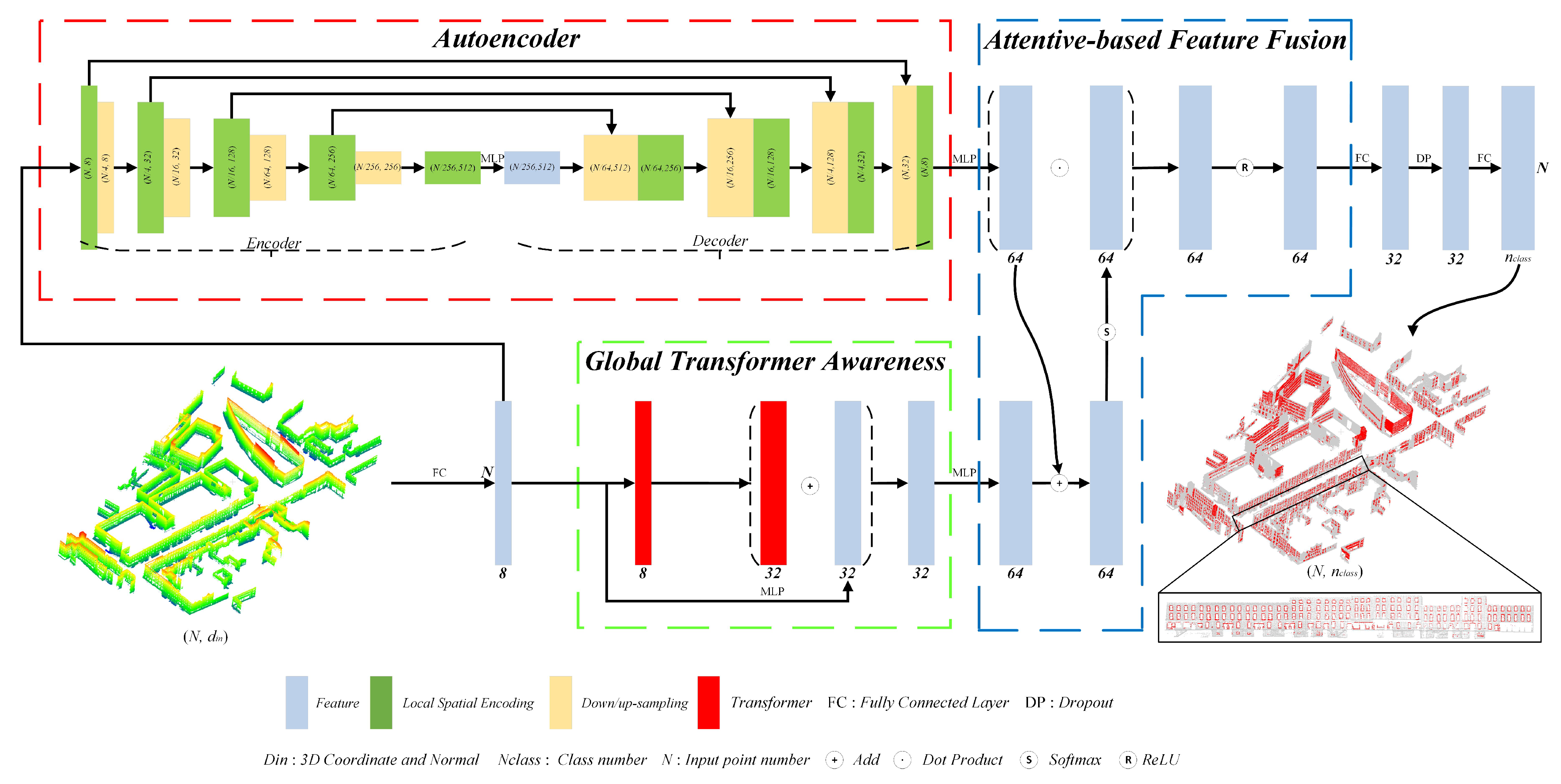
- AFGL-Net Deep Neural Network: We present AFGL-Net a deep neural network for building façade parsing. AFGL-Net uses an attentive-based feature fusion mechanism to aggregate local and global features, derived by an autoencoder and a Transformer module respectively, thereby learning enhanced and informative features to assist in solving class imbalance problem that typically occurs on building façades.
- Local Spatial Encoder: Based on the classic encoder-decoder neural network architecture, we propose an enhanced local spatial encoder by combining local position encoding and local direction encoding. The enhanced LSE encoder can easily recognize the façade component contours, e.g., window frames.
- Transformer Module: We introduce the existing Transformer module into our AFGL-Net to enhance the global/contextual feature representation. By employing these global features, AFGL-Net can perceive the small unnoticeable windows/doors by context inference from imperfect façade point clouds usually corrupted by density irregularity, outliers, and occlusions.
2. Methodology
2.1. Local Feature Aggregation
2.1.1. Autoencoder
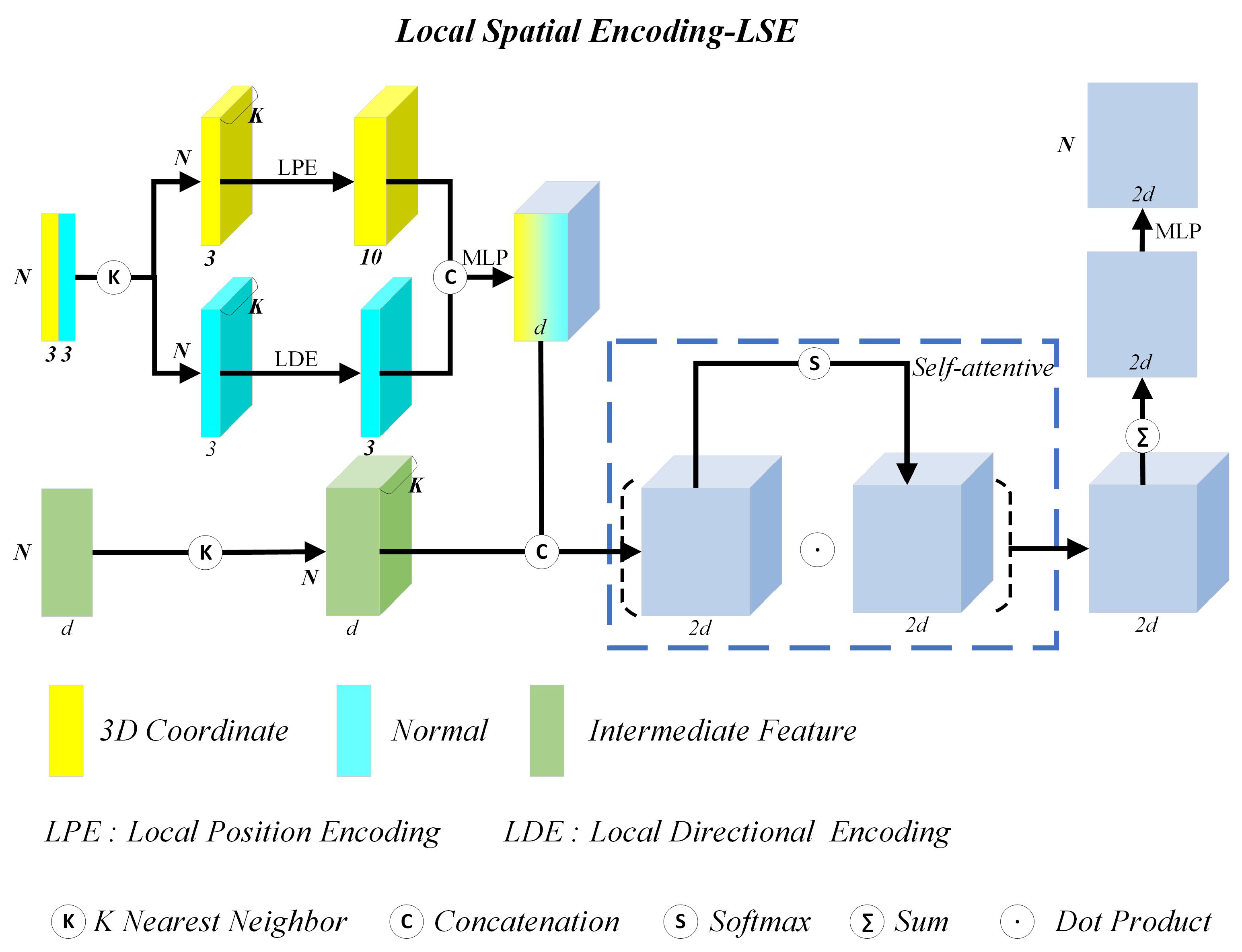
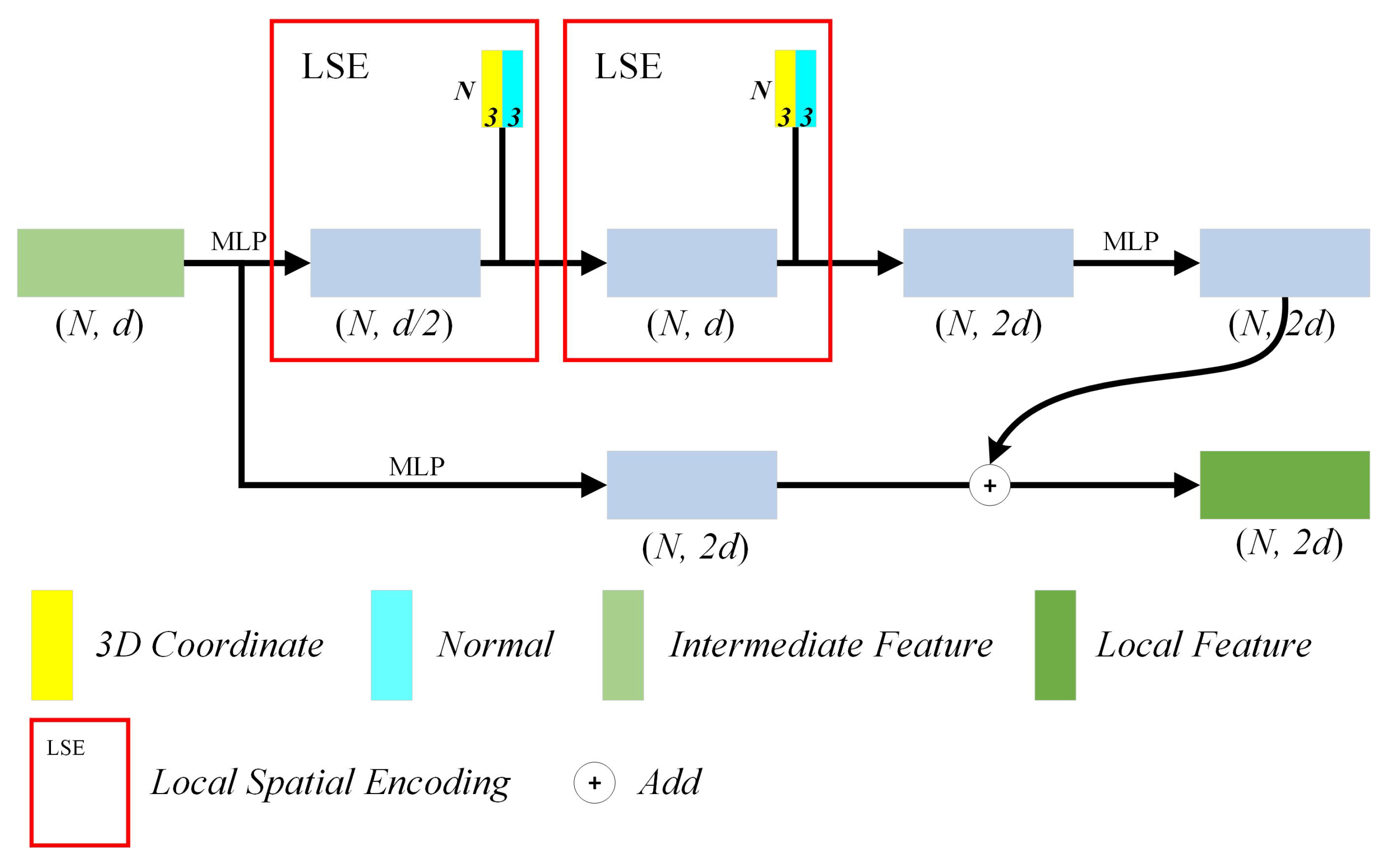
2.1.2. Local Spatial Encoding
- Each building façade point contains three types of features: positions, normal vectors and the intermediate features . We search K nearest neighbors of through KNN algorithm [39]. After that, and its K nearest neighbors are provided as input to achieve encoding of point .
- More specifically, we put and its K nearest neighbor points into LPE and LDE to achieve local position encoding and local direction encoding of point . For local position encoding of point , we put positions of and its K nearest neighbor points into LPE, and obtain a triple , where N is the number of the processed façade points at the current sampling scale. K is the number of the nearest neighbor points of , and a value of 10 is the dimension of the position feature. This position feature is composed of the x-y-z coordinates of , ’s neighbor point coordinates , the relative point coordinates between and , and the Euclidean distance between and . For local direction encoding of point , we need to put positions and normal vectors of and its K nearest neighbors into LDE, and obtain a triple , where N is the number of the processed façade points at the current sampling scale. K is the number of nearest neighbor points of , and the value of 3 is the dimension of the direction feature. The direction feature fully considers the discrepancy between ’s normal and ’s normal .
- After positional and directional encoding of point , we simply concatenate encoded position and direction features together, and input them into the shared MLP to obtain the fused features, i.e., , where d is the dimension of the fused feature channels (see hyperparameter B in Section 3.3). We concatenate the d dimensional fused feature and another d dimensional intermediate features of inputs to form a new triple . Through attentive pooling, we finally generate the informative features, denoted by a tuple .
- (1)
- Local Position Encoding
- (2)
- Local Direction Encoding
- (3)
- Local Feature Aggregation
2.1.3. Relationship with Prior Works
2.2. Global Transformer
2.3. Attention Mechanism
- Local and global feature generation: Given the input point set , we can learn local geometric features from autoencoder (see Section 2.1.1) and the global features (see Section 2.2) from two consecutive Transformers through a residual connection.
- Attention matrix construction: The local and global features and are respectively mapped onto the size by the shared MLP. After this, these two outputs are summed up to obtain the attention matrix, followed by the normalization using function.
- Feature fusion via attention mechanism: We implement dot product between the normalized attention matrix and local feature matrix to compute attention scores. Afterwards, the output vector is nonlinearly mapped to obtain the fused feature with attention scores. The whole fusion process is defined as below:where denotes the output of the attention feature. and are local and global features. is the 3D façade point, is the normalized function , and the symbol “·” denotes the dot product.
3. Performance Evaluation
3.1. Dataset Description
- (1)
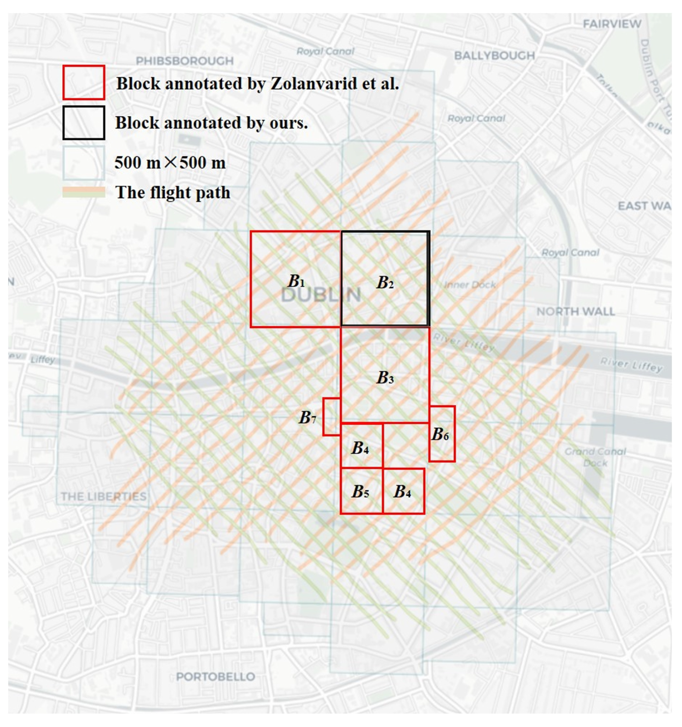
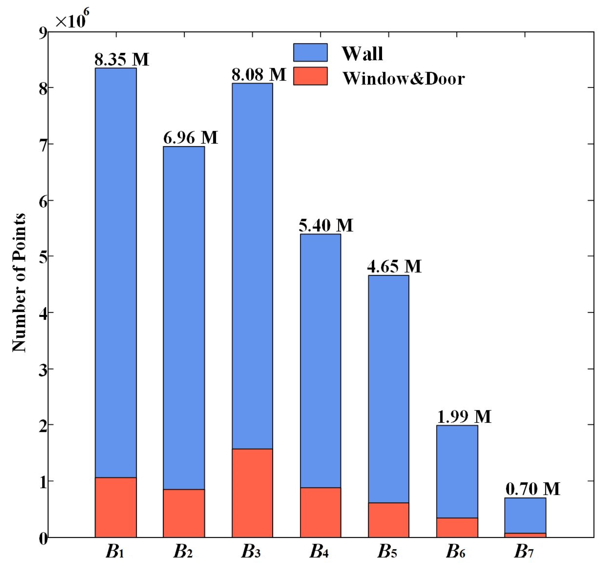
- The annotated Dublin façade point clouds
- (2)
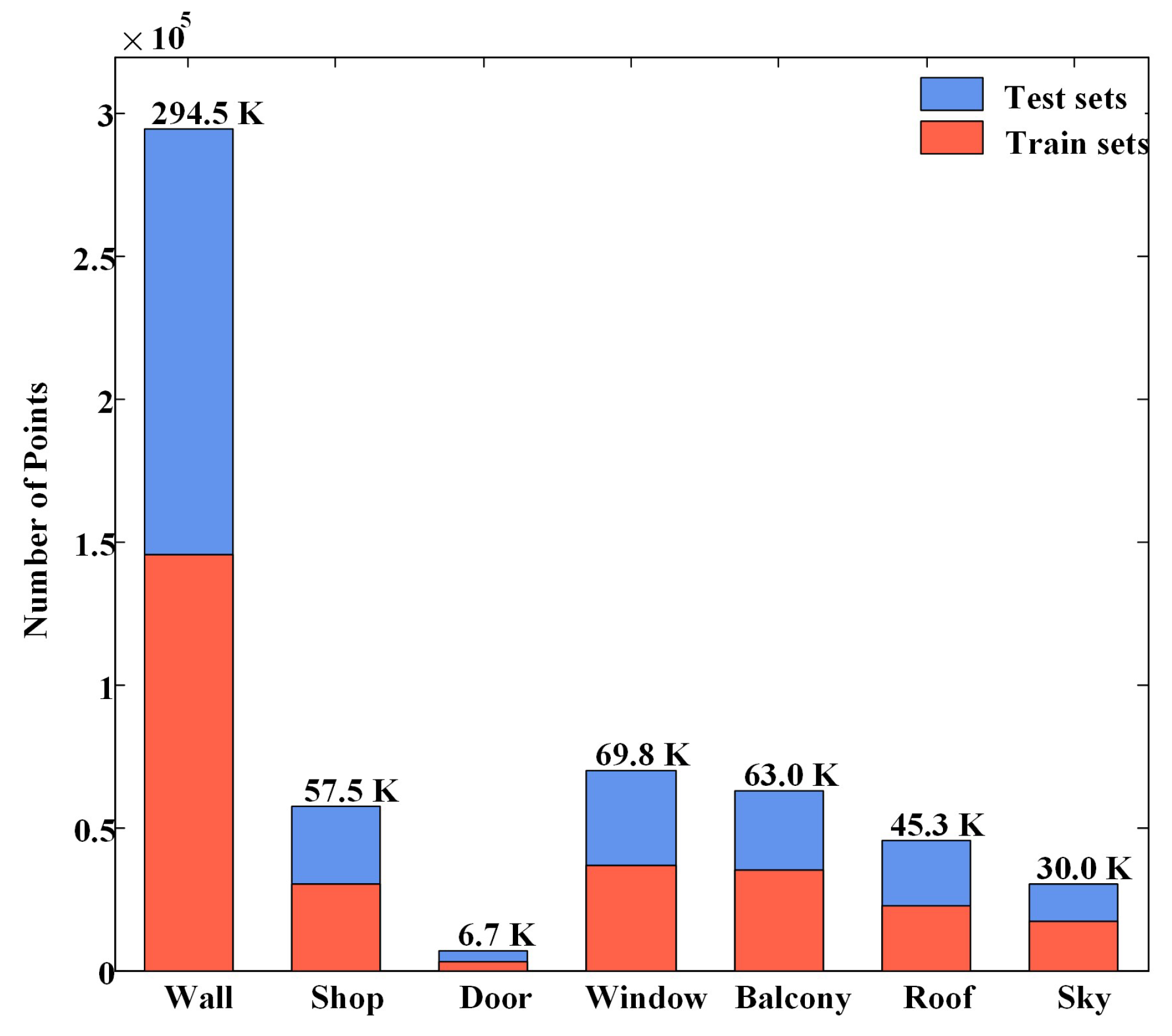
- The annotated RueMonge2014 façade points
3.2. Evaluation Metrics
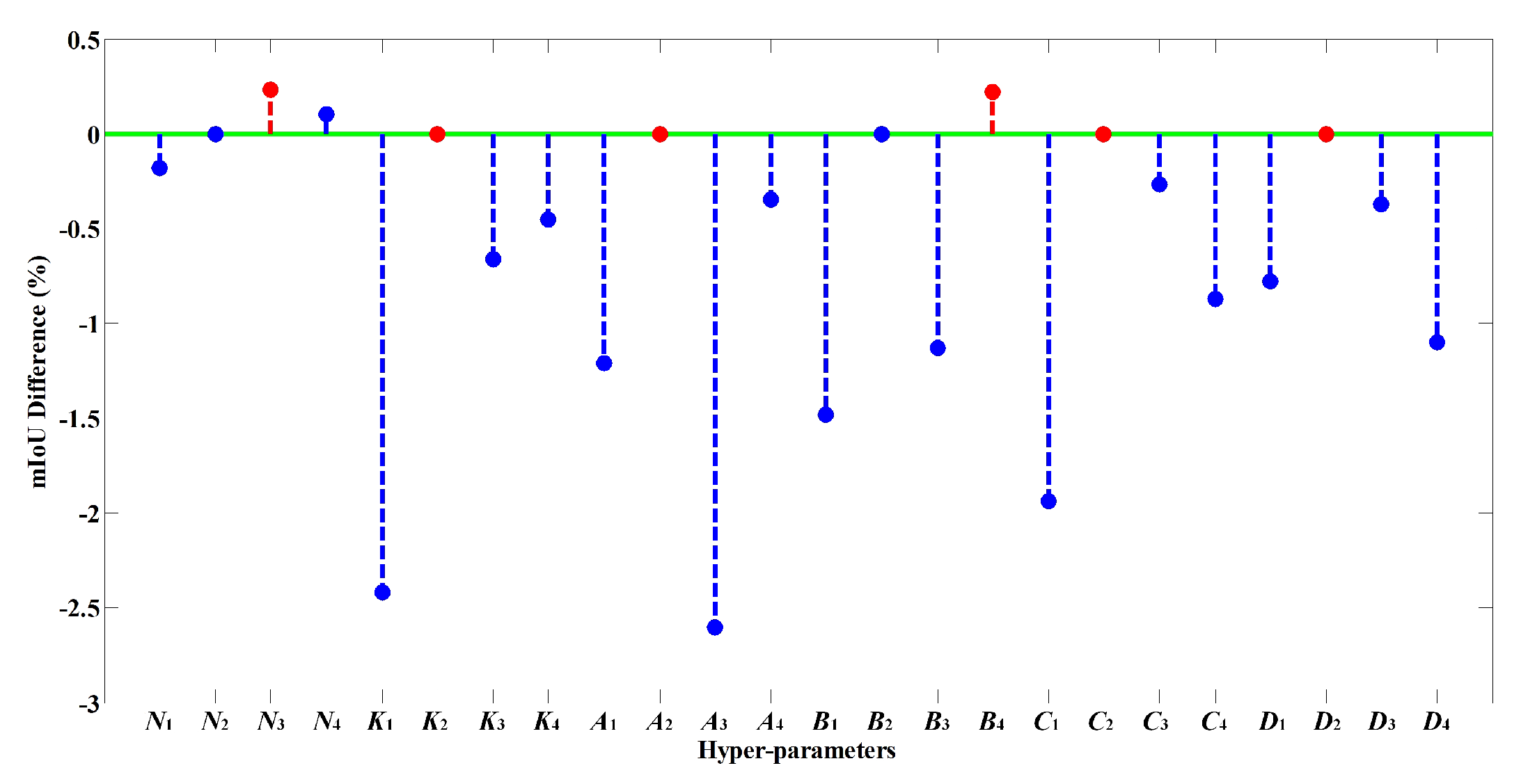
3.3. Hyperparameter Setting
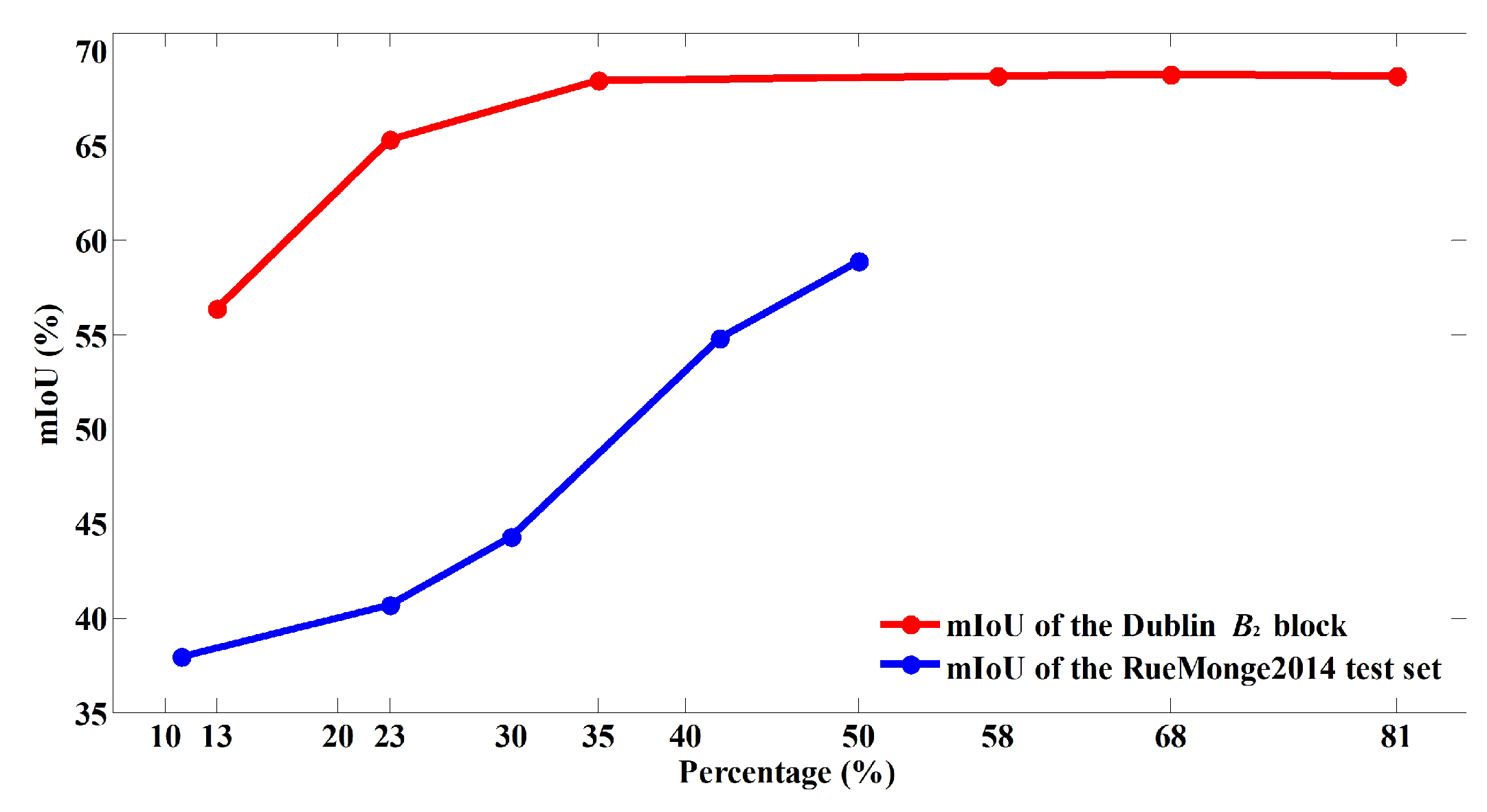
3.4. Training Size Determination
3.5. Ablation Study
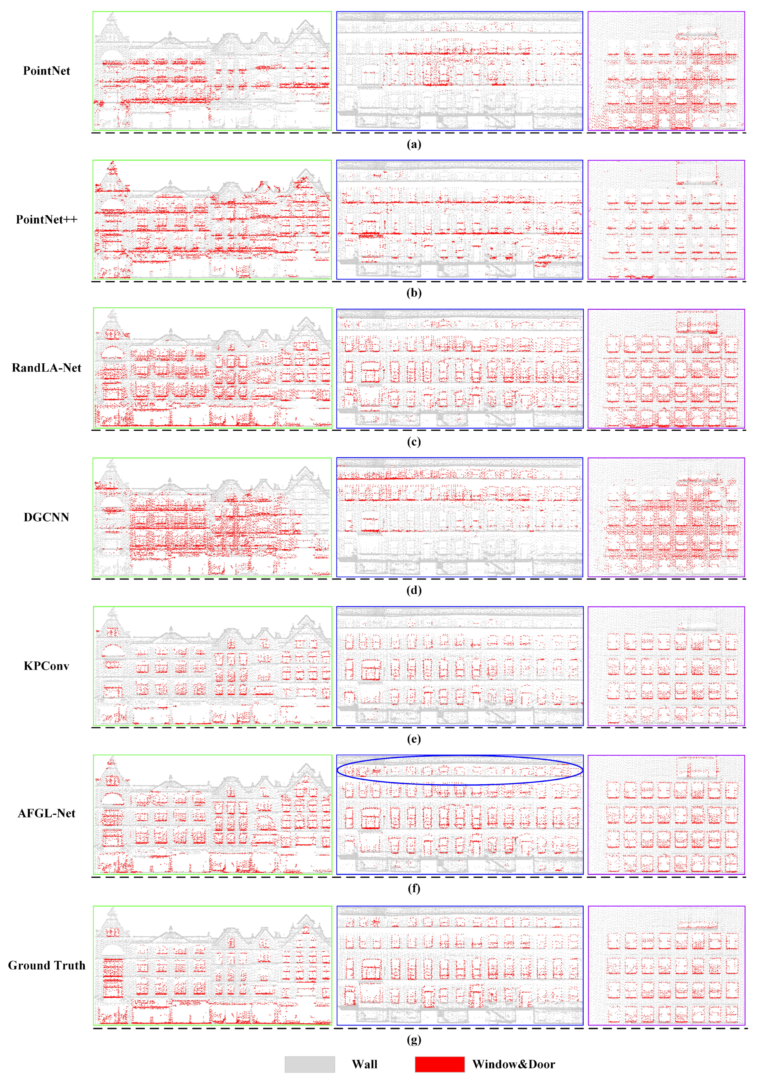
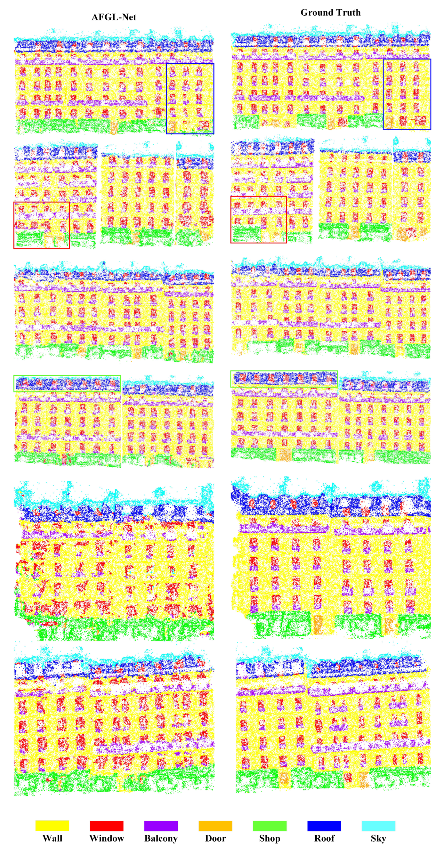
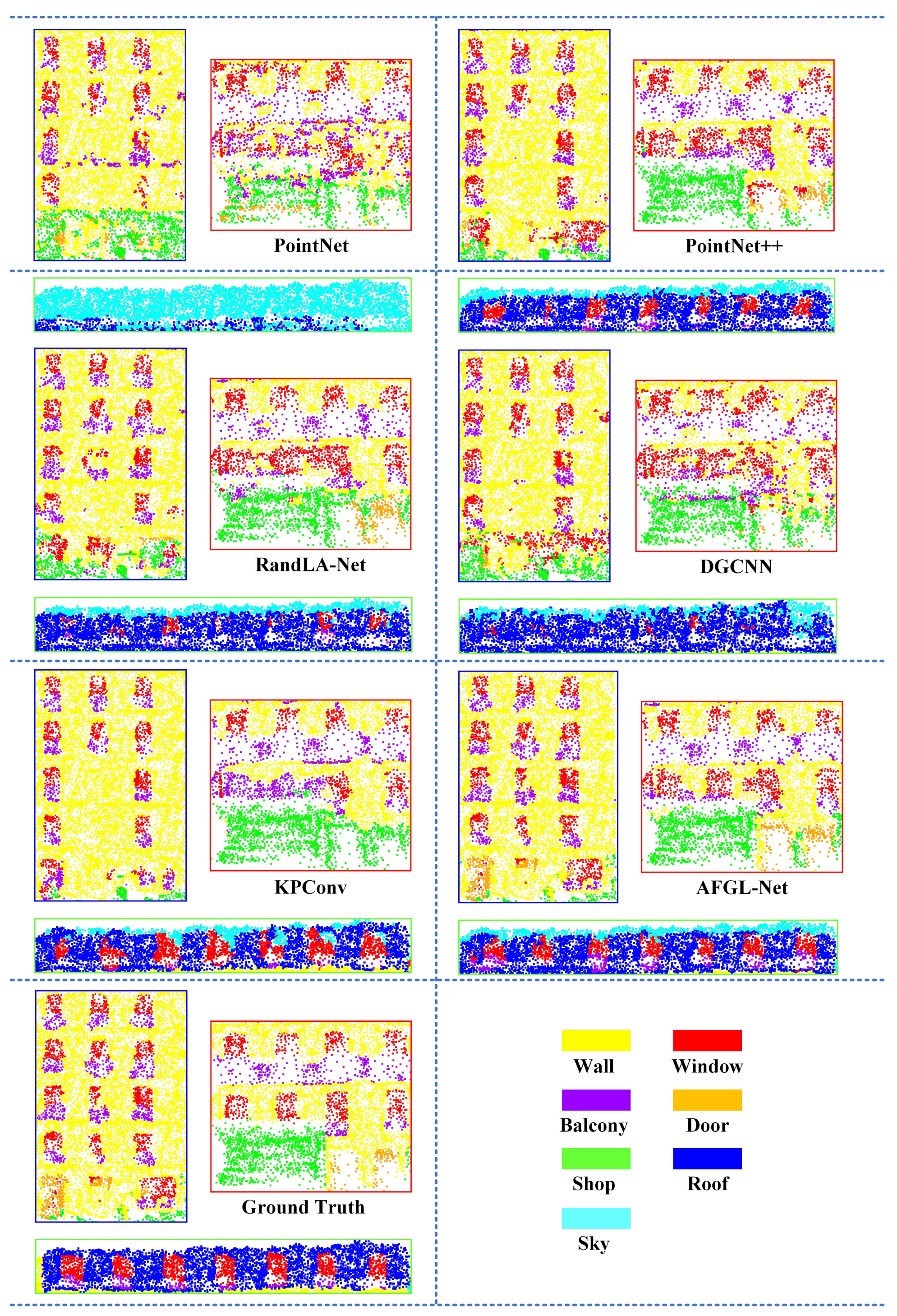
3.6. Comparison
3.7. Robustness
4. Conclusions and Suggestions for Future Research
Author Contributions
Funding
Institutional Review Board Statement
Informed Consent Statement
Data Availability Statement
Conflicts of Interest
References
- Abou Diakité, A.; Zlatanova, S. Valid space description in BIM for 3D indoor navigation. Int. J. 3-D Inf. Model. (IJ3DIM) 2016, 5, 1–17. [Google Scholar] [CrossRef] [Green Version]
- Chen, M.; Lin, H.; Liu, D.; Zhang, H.; Yue, S. An object-oriented data model built for blind navigation in outdoor space. Appl. Geogr. 2015, 60, 84–94. [Google Scholar] [CrossRef]
- Reinhart, C.F.; Davila, C.C. Urban building energy modeling–A review of a nascent field. Build. Environ. 2016, 97, 196–202. [Google Scholar] [CrossRef] [Green Version]
- Mao, B.; Ban, Y.; Harrie, L. A multiple representation data structure for dynamic visualisation of generalised 3D city models. ISPRS J. Photogramm. Remote Sens. 2011, 66, 198–208. [Google Scholar] [CrossRef]
- Verdie, Y.; Lafarge, F.; Alliez, P. LOD generation for urban scenes. ACM Trans. Graph. 2015, 34, 30. [Google Scholar] [CrossRef] [Green Version]
- Wang, R.; Peethambaran, J.; Chen, D. Lidar point clouds to 3-D urban models: A review. IEEE J. Sel. Top. Appl. Earth Obs. Remote Sens. 2018, 11, 606–627. [Google Scholar] [CrossRef]
- Du, J.; Chen, D.; Wang, R.; Peethambaran, J.; Mathiopoulos, P.T.; Xie, L.; Yun, T. A novel framework for 2.5-D building contouring from large-scale residential scenes. IEEE Trans. Geosci. Remote Sens. 2019, 57, 4121–4145. [Google Scholar] [CrossRef]
- Su, H.; Maji, S.; Kalogerakis, E.; Learned-Miller, E. Multi-view convolutional neural networks for 3d shape recognition. In Proceedings of the IEEE International Conference on Computer Vision, Santiago, Chile, 7–13 December 2015; pp. 945–953. [Google Scholar]
- Lawin, F.J.; Danelljan, M.; Tosteberg, P.; Bhat, G.; Khan, F.S.; Felsberg, M. Deep projective 3D semantic segmentation. In Proceedings of the International Conference on Computer Analysis of Images and Patterns, Ystad, Sweden, 22–24 August 2017; pp. 95–107. [Google Scholar]
- Boulch, A.; Le Saux, B.; Audebert, N. Unstructured Point Cloud Semantic Labeling Using Deep Segmentation Networks. In Proceedings of the Workshop on 3D Object Retrieval, Lyon, France, 23–24 April 2017; Volume 3. [Google Scholar]
- Maturana, D.; Scherer, S. Voxnet: A 3d convolutional neural network for real-time object recognition. In Proceedings of the 2015 IEEE/RSJ International Conference on Intelligent Robots and Systems (IROS), Hamburg, Germany, 28 September–2 October 2015; pp. 922–928. [Google Scholar]
- Graham, B.; Engelcke, M.; Van Der Maaten, L. 3d semantic segmentation with submanifold sparse convolutional networks. In Proceedings of the IEEE Conference on Computer Vision and Pattern Recognition, Salt Lake City, UT, USA, 18–23 June 2018; pp. 9224–9232. [Google Scholar]
- Riegler, G.; Osman Ulusoy, A.; Geiger, A. Octnet: Learning deep 3d representations at high resolutions. In Proceedings of the IEEE Conference on Computer Vision and Pattern Recognition, Honolulu, HI, USA, 21–26 July 2017; pp. 3577–3586. [Google Scholar]
- Klokov, R.; Lempitsky, V. Escape from cells: Deep kd-networks for the recognition of 3d point cloud models. In Proceedings of the IEEE International Conference on Computer Vision, Honolulu, HI, USA, 21–26 July 2017; pp. 863–872. [Google Scholar]
- Qi, C.R.; Su, H.; Mo, K.; Guibas, L.J. Pointnet: Deep learning on point sets for 3d classification and segmentation. In Proceedings of the IEEE Conference on Computer Vision and Pattern Recognition, Honolulu, HI, USA, 21–26 July 2017; pp. 652–660. [Google Scholar]
- Qi, C.R.; Yi, L.; Su, H.; Guibas, L.J. Pointnet++: Deep hierarchical feature learning on point sets in a metric space. arXiv 2017, arXiv:1706.02413. [Google Scholar]
- Jiang, M.; Wu, Y.; Zhao, T.; Zhao, Z.; Lu, C. Pointsift: A sift-like network module for 3d point cloud semantic segmentation. arXiv 2018, arXiv:1807.00652. [Google Scholar]
- Lowe, D.G. Distinctive image features from scale-invariant keypoints. Int. J. Comput. Vis. 2004, 60, 91–110. [Google Scholar] [CrossRef]
- Zhao, H.; Jiang, L.; Fu, C.W.; Jia, J. Pointweb: Enhancing local neighborhood features for point cloud processing. In Proceedings of the IEEE/CVF Conference on Computer Vision and Pattern Recognition, Long Beach, CA, USA, 15–20 June 2019; pp. 5565–5573. [Google Scholar]
- Li, J.; Chen, B.M.; Lee, G.H. So-net: Self-organizing network for point cloud analysis. In Proceedings of the IEEE Conference on Computer Vision and Pattern Recognition, Salt Lake City, UT, USA, 18–23 June 2018; pp. 9397–9406. [Google Scholar]
- Chiang, H.Y.; Lin, Y.L.; Liu, Y.C.; Hsu, W.H. A unified point-based framework for 3d segmentation. In Proceedings of the 2019 International Conference on 3D Vision (3DV), Quebec City, QC, Canada, 16–19 September 2019; pp. 155–163. [Google Scholar]
- Geng, X.; Ji, S.; Lu, M.; Zhao, L. Multi-Scale Attentive Aggregation for LiDAR Point Cloud Segmentation. Remote Sens. 2021, 13, 691. [Google Scholar] [CrossRef]
- Hu, Q.; Yang, B.; Xie, L.; Rosa, S.; Guo, Y.; Wang, Z.; Trigoni, N.; Markham, A. Randla-net: Efficient semantic segmentation of large-scale point clouds. In Proceedings of the IEEE/CVF Conference on Computer Vision and Pattern Recognition, Seattle, WA, USA, 13–19 June 2020; pp. 11108–11117. [Google Scholar]
- Hua, B.S.; Tran, M.K.; Yeung, S.K. Pointwise convolutional neural networks. In Proceedings of the IEEE Conference on Computer Vision and Pattern Recognition, Salt Lake City, UT, USA, 18–23 June 2018; pp. 984–993. [Google Scholar]
- Tatarchenko, M.; Park, J.; Koltun, V.; Zhou, Q.Y. Tangent convolutions for dense prediction in 3d. In Proceedings of the IEEE Conference on Computer Vision and Pattern Recognition, Salt Lake City, UT, USA, 18–23 June 2018; pp. 3887–3896. [Google Scholar]
- Zhang, Z.; Hua, B.S.; Yeung, S.K. Shellnet: Efficient point cloud convolutional neural networks using concentric shells statistics. In Proceedings of the IEEE/CVF International Conference on Computer Vision, Seoul, Korea, 27 October–2 November 2019; pp. 1607–1616. [Google Scholar]
- Li, Y.; Bu, R.; Sun, M.; Wu, W.; Di, X.; Chen, B. Pointcnn: Convolution on x-transformed points. Adv. Neural Inf. Process. Syst. 2018, 31, 820–830. [Google Scholar]
- Thomas, H.; Qi, C.R.; Deschaud, J.E.; Marcotegui, B.; Goulette, F.; Guibas, L.J. Kpconv: Flexible and deformable convolution for point clouds. In Proceedings of the IEEE/CVF International Conference on Computer Vision, Long Beach, CA, USA, 15–20 June 2019; pp. 6411–6420. [Google Scholar]
- Komarichev, A.; Zhong, Z.; Hua, J. A-cnn: Annularly convolutional neural networks on point clouds. In Proceedings of the IEEE/CVF Conference on Computer Vision and Pattern Recognition, Long Beach, CA, USA, 15–20 June 2019; pp. 7421–7430. [Google Scholar]
- Wang, Y.; Sun, Y.; Liu, Z.; Sarma, S.E.; Bronstein, M.M.; Solomon, J.M. Dynamic Graph Cnn for Learning on Point Clouds; ACM: New York, NY, USA, 2019; Volume 38, pp. 1–12. [Google Scholar]
- Te, G.; Hu, W.; Zheng, A.; Guo, Z. Rgcnn: Regularized graph cnn for point cloud segmentation. In Proceedings of the 26th ACM International Conference on Multimedia, Seoul, Korea, 22–26 October 2018; pp. 746–754. [Google Scholar]
- Wang, L.; Huang, Y.; Hou, Y.; Zhang, S.; Shan, J. Graph attention convolution for point cloud semantic segmentation. In Proceedings of the IEEE/CVF Conference on Computer Vision and Pattern Recognition, Long Beach, CA, USA, 15–20 June 2019; pp. 10296–10305. [Google Scholar]
- Landrieu, L.; Simonovsky, M. Large-scale point cloud semantic segmentation with superpoint graphs. In Proceedings of the IEEE Conference on Computer Vision and Pattern Recognition, Salt Lake City, UT, USA, 18–23 June 2018; pp. 4558–4567. [Google Scholar]
- Zhang, S.; Tong, H.; Xu, J.; Maciejewski, R. Graph convolutional networks: A comprehensive review. Comput. Soc. Netw. 2019, 6, 1–23. [Google Scholar] [CrossRef] [Green Version]
- Vaswani, A.; Shazeer, N.; Parmar, N.; Uszkoreit, J.; Jones, L.; Gomez, A.N.; Kaiser, Ł.; Polosukhin, I. Attention is all you need. In Proceedings of the Advances in Neural Information Processing Systems, Long Beach, CA, USA, 4–9 December 2017; pp. 5998–6008.
- Zolanvari, S.; Ruano, S.; Rana, A.; Cummins, A.; da Silva, R.E.; Rahbar, M.; Smolic, A. DublinCity: Annotated LiDAR point cloud and its applications. arXiv 2019, arXiv:1909.03613. [Google Scholar]
- Riemenschneider, H.; Bódis-Szomorú, A.; Weissenberg, J.; Van Gool, L. Learning where to classify in multi-view semantic segmentation. In Proceedings of the European Conference on Computer Vision, Zurich, Switzerland, 6–12 September 2014; pp. 516–532. [Google Scholar]
- Ronneberger, O.; Fischer, P.; Brox, T. U-net: Convolutional networks for biomedical image segmentation. In Proceedings of the International Conference on Medical Image Computing and Computer-Assisted Intervention, Munich, Germany, 5–9 October 2015; pp. 234–241. [Google Scholar]
- Fix, E.; Hodges, J.L. Discriminatory analysis. Nonparametric discrimination: Consistency properties. Int. Stat. Rev. Int. De Stat. 1989, 57, 238–247. [Google Scholar] [CrossRef]
- Rusu, R.B.; Blodow, N.; Marton, Z.C.; Beetz, M. Aligning point cloud views using persistent feature histograms. In Proceedings of the 2008 IEEE/RSJ International Conference on Intelligent Robots and Systems, Nice, France, 22–26 September 2008; pp. 3384–3391. [Google Scholar]
- Rusu, R.B.; Blodow, N.; Beetz, M. Fast point feature histograms (FPFH) for 3D registration. In Proceedings of the 2009 IEEE International Conference on Robotics and Automation, Kobe, Japan, 12–17 May 2009; pp. 3212–3217. [Google Scholar]
- Laefer, D.F.; Abuwarda, S.; Vo, A.V.; Truong-Hong, L.; Gharibi, H. 2015 Aerial Laser and Photogrammetry Survey of Dublin City Collection Record; Technical Report; New York University: New York, NY, USA, 2017. [Google Scholar]


| Building Façade | Window & Door | Wall |
|---|---|---|
| #Pts | 5,375,755 | 30,749,496 |
| Percentage | 14.88% | 85.12% |
| Hyperparameters | Scheme 1 | Scheme 2 (Baseline Parameter) | Scheme 3 | Scheme 4 |
|---|---|---|---|---|
| N | 4096 | 8192 | 16,384 | 32,768 |
| K | 8 | 16 | 24 | 32 |
| A | 3 | 4 | 5 | 6 |
| B | (8-32-64-128) | (16-64-128-256) | (32-128-256-512) | (64-256-512-1024) |
| C | 1 | 2 | 3 | 4 |
| D | (4-16) | (8-32) | (16-64) | (32-128) |
| Hyperparameters | Scheme 1 | Scheme 2 ( Baseline Parameter) | Scheme 3 |
|---|---|---|---|
| N | 1024 | 2048 | 4096 |
| K | 8 | 16 | 24 |
| A | 3 | 4 | 5 |
| B | (8-32-64-128) | (16-64-128-256) | (32-128-256-512) |
| C | 1 | 2 | 3 |
| D | (4-16) | (8-32) | (16-64) |
| Training Set | Window & Door IoU (%) | Wall IoU (%) | mIoU (%) | OA (%) |
|---|---|---|---|---|
| B5 (12.88%) | 32.37 | 80.39 | 56.38 | 82.08 |
| B1 (23.11%) | 42.34 | 88.25 | 65.29 | 89.19 |
| B4 ∼B7 (35.27%) | 47.46 | 89.42 | 68.44 | 90.30 |
| B3∼B7 (57.63%) | 48.49 | 88.86 | 68.67 | 89.92 |
| B1; B3∼B4; B6∼B7 (67.86%) | 48.57 | 88.91 | 68.74 | 89.96 |
| B1; B3∼B7 (80.74%) | 48.55 | 88.88 | 68.72 | 89.94 |
| Configurations | Window & Door IoU (%) | Wall IoU (%) | mIoU (%) | OA (%) | |
|---|---|---|---|---|---|
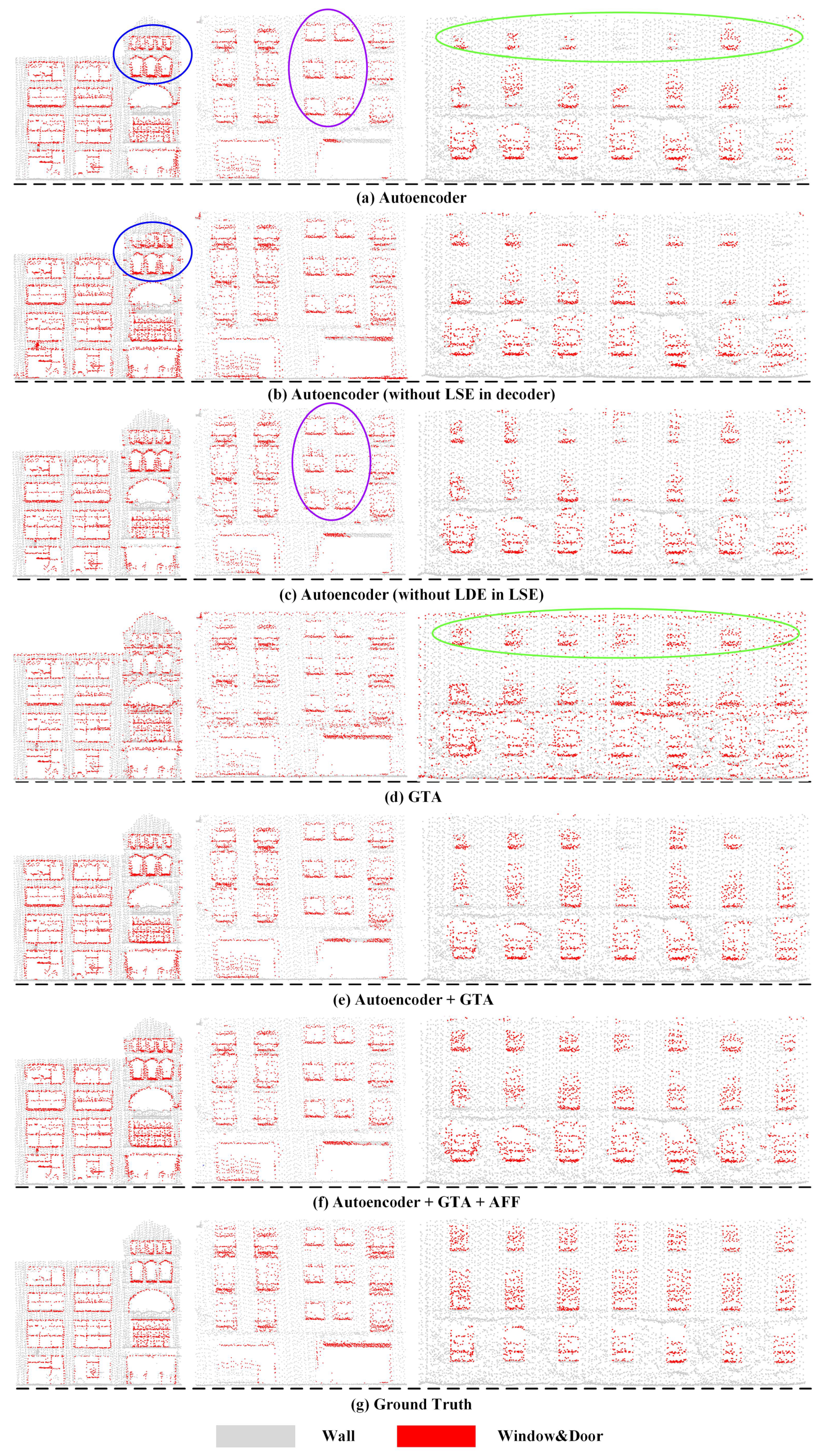
| (a) | Autoencoder | 45.85 | 86.12 | 65.98 | 87.58 |
| (b) | Autoencoder (without LSE in decoder) | 43.76 | 84.47 | 64.12 | 86.15 |
| (c) | Autoencoder (without LDE in LSE) | 44.31 | 86.48 | 65.40 | 87.79 |
| (d) | GTA | 26.22 | 77.48 | 51.85 | 79.15 |
| (e) | Autoencoder + GTA | 46.17 | 85.59 | 65.88 | 87.17 |
| (f) | Autoencoder + GTA + AFF | 46.80 | 87.12 | 66.96 | 88.43 |
| Methods | Window & Door IoU (%) | Wall IoU (%) | mIoU (%) | OA (%) | Training Time (min) | Testing Time (min) |
|---|---|---|---|---|---|---|
| PointNet | 20.14 | 78.20 | 49.17 | 79.34 | 86.75 | 2.23 |
| PointNet++ | 33.85 | 79.76 | 56.81 | 81.66 | 231.72 | 5.35 |
| RandLA-Net | 43.64 | 84.32 | 63.98 | 86.02 | 161.67 | 3.93 |
| DGCNN | 28.28 | 79.41 | 53.85 | 80.97 | 170.90 | 3.83 |
| KPConv | 42.79 | 88.86 | 65.83 | 89.72 | 194.44 | 6.02 |
| Ours | 47.06 | 86.97 | 67.02 | 88.32 | 253.95 | 4.42 |
| Methods | Wall IoU (%) | Sky IoU (%) | Balcony IoU (%) | Window IoU (%) | Door IoU (%) | Shop IoU (%) | Roof IoU (%) | mIoU (%) | OA (%) | Training Time (min) | Testing Time (min) |
|---|---|---|---|---|---|---|---|---|---|---|---|
| PointNet | 48.09 | 45.39 | 24.41 | 24.12 | 12.63 | 47.52 | 33.62 | 33.68 | 55.33 | 49.90 | 0.33 |
| PointNet++ | 73.47 | 63.42 | 51.44 | 45.49 | 16.19 | 57.94 | 54.48 | 51.78 | 76.81 | 153.02 | 0.88 |
| RandLA-Net | 74.81 | 70.67 | 54.15 | 48.64 | 21.57 | 59.29 | 60.89 | 55.72 | 78.68 | 69.05 | 1.31 |
| DGCNN | 67.45 | 64.71 | 38.89 | 38.32 | 18.53 | 57.60 | 58.81 | 49.19 | 72.19 | 170.20 | 0.40 |
| KPConv | 74.41 | 62.74 | 39.26 | 40.44 | 6.34 | 43.95 | 58.96 | 46.59 | 75.69 | 225.45 | 0.97 |
| Ours | 77.28 | 70.07 | 54.03 | 53.31 | 37.01 | 64.08 | 62.80 | 59.80 | 80.71 | 77.12 | 1.50 |
Publisher’s Note: MDPI stays neutral with regard to jurisdictional claims in published maps and institutional affiliations. |
© 2021 by the authors. Licensee MDPI, Basel, Switzerland. This article is an open access article distributed under the terms and conditions of the Creative Commons Attribution (CC BY) license (https://creativecommons.org/licenses/by/4.0/).
Share and Cite
Chen, D.; Xiang, G.; Peethambaran, J.; Zhang, L.; Li, J.; Hu, F. AFGL-Net: Attentive Fusion of Global and Local Deep Features for Building Façades Parsing. Remote Sens. 2021, 13, 5039. https://doi.org/10.3390/rs13245039
Chen D, Xiang G, Peethambaran J, Zhang L, Li J, Hu F. AFGL-Net: Attentive Fusion of Global and Local Deep Features for Building Façades Parsing. Remote Sensing. 2021; 13(24):5039. https://doi.org/10.3390/rs13245039
Chicago/Turabian StyleChen, Dong, Guiqiu Xiang, Jiju Peethambaran, Liqiang Zhang, Jing Li, and Fan Hu. 2021. "AFGL-Net: Attentive Fusion of Global and Local Deep Features for Building Façades Parsing" Remote Sensing 13, no. 24: 5039. https://doi.org/10.3390/rs13245039
APA StyleChen, D., Xiang, G., Peethambaran, J., Zhang, L., Li, J., & Hu, F. (2021). AFGL-Net: Attentive Fusion of Global and Local Deep Features for Building Façades Parsing. Remote Sensing, 13(24), 5039. https://doi.org/10.3390/rs13245039