Abstract
As an all-weather and all-day remote sensing image data source, SAR (Synthetic Aperture Radar) images have been widely applied, and their registration accuracy has a direct impact on the downstream task effectiveness. The existing registration algorithms mainly focus on small sub-images, and there is a lack of available accurate matching methods for large-size images. This paper proposes a high-precision, rapid, large-size SAR image dense-matching method. The method mainly includes four steps: down-sampling image pre-registration, sub-image acquisition, dense matching, and the transformation solution. First, the ORB (Oriented FAST and Rotated BRIEF) operator and the GMS (Grid-based Motion Statistics) method are combined to perform rough matching in the semantically rich down-sampled image. In addition, according to the feature point pairs, a group of clustering centers and corresponding images are obtained. Subsequently, a deep learning method based on Transformers is used to register images under weak texture conditions. Finally, the global transformation relationship can be obtained through RANSAC (Random Sample Consensus). Compared with the SOTA algorithm, our method’s correct matching point numbers are increased by more than 2.47 times, and the root mean squared error (RMSE) is reduced by more than 4.16%. The experimental results demonstrate that our proposed method is efficient and accurate, which provides a new idea for SAR image registration.
1. Introduction
Synthetic aperture radar (SAR) has the advantages of working in all weather, at all times, and having strong penetrability. SAR image processing is developing rapidly in civilian and military applications. There are many practical scenarios for the joint processing and analysis of multiple remote sensing images, such as data fusion [1], change detection [2], and pattern recognition [3]. The accuracy of the image matching affects the performance of the above downstream tasks. However, SAR image acquisition conditions are diverse, such as different polarizations, incident angles, imaging methods, time phases, and so on. At the same time, defocusing problems caused by motion errors degrade the image quality. Besides this, the time and spatial complexity of traditional methods are unacceptable for large images. Thus, for the mass of scenes where multiple SAR images are processed simultaneously, SAR image registration is a real necessity. The nonlinear distortion and inherent speckle noise of SAR images leave wide-swath SAR image registration as a knot to be solved.
The geographical alignment of two SAR images, under different imaging conditions, is based on the mapping model, which is usually solved by the relative relationship of the corresponding parts from images. The two images are reference images and sensed images to be registered. Generally speaking, conventional geometric transformation models include affine, projection, rigid body, and nonlinear transformation models. In this paper, we focus on the most pervasive affine transformation model.
The registration techniques in the Computer Vision (CV) field have continued to spring up for decades. The existing normal registration methods can be divided mainly into traditional algorithms and learning-based algorithms. The traditional methods mainly include feature-based and region-based methods. The region-based method finds the best transformation parameters based on the maximum similarity coefficient, and includes mutual information methods [4], Fourier methods [5], and cross-correlation methods [6,7]. Stone et al. [5] presented a Fourier-based algorithm to solve translations and uniform changes of illumination in aerial photos. Recently, in the field of SAR image registration, Luca et al. [7] used cross-correlation parabolic interpolation to refine the matching results. This series of methods only use plain gray information and risk mismatch under speckle noise and radiation variation.
Another major class of registration techniques in the CV field is the feature-based method. It searches for geometric mappings such as points, lines, contours, and regional features based on the stable feature correspondences across two images. The most prevalent method is SIFT (Scale Invariant Feature Transform) [8]. SIFT has been widely used in the field of image registration due to the following invariances: rotation, scale, grayscale, and so on. PCA-SIFT (Principal Component Analysis-SIFT) [9] applies dimensionality reduction to SIFT descriptors to improve the matching efficiency. Slightly different from the classical CV field, a series of unique image registration methods appear in the SAR image processing field. Given the characteristics of SAR speckle noise, SAR-SIFT [10] adopts a new method of gradient calculation and feature descriptor generation to improve the SAR image registration performance. KAZE-SAR [11] uses the nonlinear diffusion filtering method KAZE [12] to build the scale space. Xiang [13] proposed a method to match large SAR images with optical images. To be specific, the method combines dilated convolutional features with epipolar-oriented phase correlation to reduce horizontal errors, and then fine-tunes the matching part. Feature-based methods are more flexible and effective; as such, they are more practical under complex spatial change. Coherent speckle noise has consequences on the conventional method’s precision, and the traditional matching approach fails to achieve the expected results under complex and varied scenarios.
Deep learning [14] (DL) has exploded in CV fields over the past decade. With strong abilities of feature extraction and characterization, deep learning is in wide usage across remote sensing scenarios, including classification [15], detection [16], image registration [17], and change detection [18]. More and more methods [19,20] use learning-based methods in the registration of the CV field. He et al. [19] proposed a Siamese CNN (Convolutional Neural Networks) to evaluate the similarity of patch pairs. Zheng et al. [20] proposed SymReg-GAN, which achieves good results in medical image registration by using a generator that predicts the geometric transformation between images, and a discriminator that distinguishes the transformed images from the real images. Specific to the SAR image (remote sensing image) registration field, Li et al. [21] proposed a RotNET to predict the rotation relationship between two images. Mao et al. [22] proposed a multi-scale fused deep forest-based SAR image registration method. Luo et al. [23] used pre-trained deep residual neural features extracted from CNN for registration. The CMM-Net (cross modality matching net) [24] used CNN to extract high-dimensional feature maps and build descriptors. DL often requires large training datasets. Unlike optical natural images, it is difficult to accurately label SAR images due to the influence of noise. In addition, most DL-based SAR image registration studies generally deal with small image blocks with a fixed size, but in practical applications, wide-swath SAR images cannot be directly matched.
As was outlined earlier in this article, Figure 1 lists some of the registration methods for SAR (remote sensing) image domains. Although many SAR image registration methods exist, there are still some limitations:
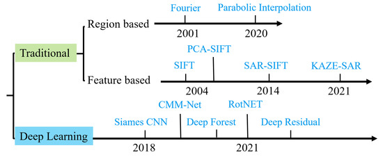
Figure 1.
Remote sensing image registration milestones in the last two decades.
- Feature points mainly exist in the strong corner and edge areas, and there are not enough matching point pairs in weak texture areas.
- Due to the special gradient calculation and feature space construction method, the traditional method runs slowly and consumes a lot of memory.
- The existing SAR image registration methods mainly rely on the CNN structure, and lack a complete relative relationship between their features due to the receptive field’s limitations.
Based on the above analysis, this paper proposes a wide-swath SAR image fine-level registration framework that combines traditional methods and deep learning. The experimental results show that, compared with the state of the art, the proposed method can obtain better matching results. Under the comparison and analysis of the matching performance in different data sources, the method in this paper is more effective and robust for SAR image registration.
The general innovations of this paper are as follows:
- A CNN and Transformer hybrid approach is proposed in order to accurately register SAR images through a coarse-to-fine form.
- A stable partition framework from the full image to sub-images is constructed; in this method, the regions of interest are selected in pairs.
The remainder of this paper is organized as follows. In Section 2. Methods, the proposed framework of SAR image registration and the learning-based sub-image matching method are discussed in detail. In Section 3. Experimental Results and Analyses, specified experiments, as well as quantitative and qualitative results, are given. In Section 4. Discussion, the conclusion is provided.
2. Methods
In this study, we propose a phased SAR image registration framework that combines traditional and deep learning methods. The framework is illustrated in Figure 2; the proposed method mainly consists of four steps. First, the ORB [25] and GMS [26] are used to obtain the coarse registration result via the downsampled original image. Second, K-means++ [27] select cluster centers of registration points from the previous step, and a series of corresponding original-resolution image slices are obtained. Third, we register the above image pairs through deep learning. The fourth step is to integrate the point pair subsets and obtain the final global transformation result after RANSAC [28].
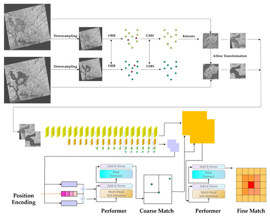
Figure 2.
The pipeline of the proposed method.
As a starting point for our work, we first introduce the existing deep learning mainstream.
2.1. Deep Learning-Related Background
As AlexNet [29] won first place in 2012 ImageNet, deep learning had begun to play a leading role in CV, NLP (natural language processing), and other fields. The current mainstream of deep learning includes two categories: CNN and Transformer. CNN does well in the extraction of local information from two-dimensional data, such as images. Because the deep neural network can extract key features from massive data, deep CNN is performed outstandingly in image classification [30], detection [16,31], and segmentation [32].
Corresponding to text and other one-dimensional sequence data, currently, the most widely used processing method is Transformer [33], which solves the long-distance relying problem using a unique self-attention mechanism. It is sweeping NLP, CV, and related fields.
Deep learning has been widely used in SAR image processing over the past few years. For example, Hou et al. [16] proposed ship classification using CNN in an SAR ship dataset. Guo et al. [31] applied an Attention Pyramid Network for aircraft detection. Transformer is also used in recognition [34], detection [35] and segmentation [36]. LoFTR (Local Feature TRansformer) [37] has been proposed as a coarse-to-fine image matching method based on Transformers. However, to our knowledge, Transformer has not been applied to SAR image registration. Inspired by [37], in this article we use Transformer and CNN to improve the performance of SAR image registration.
The method proposed in this paper is mainly inspired by LoFTR. The initial consideration is that in the SAR image registration scene, due to the weak texture information, traditional CV registration methods based on gradient, statistical information, and other classical methods cannot obtain enough matching point pairs. LoFTR adopts a two-stage matching mechanism and features coding with Transformer, such that each position in the feature map contains the global information of the whole image. It works well in natural scenes, and also has a good matching effect even in flat areas with weak texture information. However, considering that SAR images have weaker texture information than optical images, it is difficult to obtain sufficient feature information.
In order to obtain more matching feature point pairs and give consideration to model complexity and algorithm accuracy, this paper adopts several modification schemes for SAR image scenes. (1) Feature Pyramid Network is used as a feature extraction network in LoFTR; in this paper, an advanced convolutional neural network, is adopted as a feature extraction part in order to obtain more comprehensively high- and low-resolution features with feature fusion. (2) This paper analyzes the factors that affect the number of matching point pairs, and finds that the size of the low-resolution feature map has an obvious direct impact on the number of feature point pairs. The higher the resolution, the higher the number of correct matching points that are finally extracted. Therefore, (1/2,1/5) resolution is adopted to replace the original (1/2,1/8) or (1/4,1/16); such a change leads to the number of matching point pairs increasing significantly. (3) In order to further reduce the algorithm complexity and improve the algorithm speed, this paper combines the advanced linear time complexity method to encode features, such that the location features at the specific index of the feature map can be weighted by the full image information, which can further improve the efficiency while ensuring the algorithm accuracy. The detailed expansion and analysis of the above parts are in the following sections.
2.2. Rough Matching of the Down-Sampled Image
The primary reasons that the traditional matching methods SIFT and SURF (Speeded-Up Robust Features) [38] cannot be applied directly to SAR images are the serious coherent speckle noise and the weak discontinuous texture. It is often impossible to obtain sufficient matching points on original-resolution SAR images by the traditional method. At the same time, the semantic information of the original-size image is relatively scarce. Therefore, we do not simply use traditional methods to process the original image. Considering that the down-sampled image is similar to a high-level feature map in deep CNN with rich semantic information, we use the down-sampled image (the rate is 10 almost) to perform rough pre-matching, as shown in Figure 3. The most representative method is SIFT. However, it runs slowly, especially for large images. The ORB algorithm is two orders of magnitude more rapid [25] than SIFT. ORB is a stable and widely used feature point detection description method.
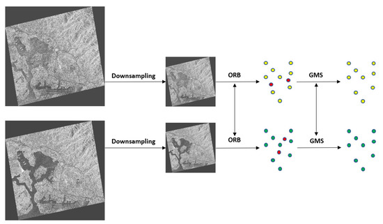
Figure 3.
The pipeline of rough matching.
ORB combines and improves the FAST (Features from Accelerated Segment Test) [39] keypoint detector and the BRIEF (Binary Robust Independent Elementary Features) [40] descriptor. FAST’s idea is that if the pixel’s gray is distinguished from the surrounding neighborhood (i.e., it exceeds the threshold value), it may be a feature point. To be specific, FAST uses a neighborhood of 16 pixels to select the initial candidate points. Non-maximum suppression is used to eliminate the adjacent points. The gaussian blurring of different scales is performed on the image in order to achieve scale invariance.
The intensity weighted sum of a patch is defined as the centroid, and the orientation is obtained via the angle between the current point and the centroid. Orientation invariance can be enhanced by calculating moments. BRIEF is a binary coded descriptor that uses binary and bit XOR operations to speed up the establishment of feature descriptors and reduce the time for feature matching. Steered BRIEF and rBRIEF are applied for rotation invariance and distinguishability, respectively. Overall, FAST accelerates the feature point detection, and BRIEF reduces the spatial redundancy.
GMS is applied after ORB to obtain more matching point pairs; here is a brief description. If the images and , respectively, have N and M feature points, the set of feature points is written as {M, N}, the feature matching pair in the corresponding two images is , , and a and b are the neighborhoods of the feature points from two images and . For a correct matching point pair, there are more matching points as support for its correctness. For the matching pair , is used to represent the support of its neighboring feature points, where is the number of matching pairs in the neighborhood of . Because the matching of each feature point is independent, it can be considered that approximately obeys the binomial distribution, and can be defined as
n is the average number of feature points in each small neighborhood. Let be one of the supporting features belonging to region a. is the probability that region b includes the nearest neighbor of , and similarly, can be defined, and and can be obtained by the following formulae:
, , and correspond to events: is correctly matched, is incorrectly matched, and ’s matching point appears in region b. m represents the number of all of the feature points in region b in image , and M represents the number of all of the feature points in image . In order to further improve the discriminative ability, the GMS algorithm uses the multi-neighborhood model to replace the single-neighborhood model:
K is the number of small neighborhoods near the matching point, is the number of matching pairs in the two matching neighborhoods, and can be extended to
According to statistics, an evaluation score P is defined to measure the ability of the function to discriminate between right and wrong matches, as follows:
Among them, and are the standard deviations of in positive and false matches, respectively, and and are the mean values, respectively. It can be seen from formula (5) that the greater the feature points’ number, the higher the matching accuracy. If we set for grid pair {i,j} and for the threshold, then {i,j} is regarded as a correctly matched grid pair when .
In order to reduce the computational complexity, GMS replaces the circular neighborhood with a non-overlapping square grid to speed up ’s calculation. Experiments have shown that when the number of feature points is 10,000, the image is divided into a 20 × 20 grid. The GMS algorithm scales the grid size for image size invariance, introduces a motion kernel function to process the image, and converts the rotation changes into the rearrangement of the corresponding neighborhood grid order to ensure rotation invariance.
2.3. Sub-Image Acquisition from the Cluster Centers
The existing image matching methods mostly apply to small-size images, which have lower time and storage requirements. Although some excellent methods can reach sub-pixels in local areas, they cannot be extended to a large scale due to their unique gradient calculation method and scale-space storage. Take the representative algorithm SAR-SIFT, for example; its time and memory consumption vary with the size, as shown in Figure 4, and when the image size reaches 5000–10,000 pixels or more, the memory reaches a certain peak. This computational consumption is unacceptable for ordinary desktop computers. The test experiment here was performed on high-performance workstations. Even so, the memory consumption caused by the further expansion of the image size is unbearable.
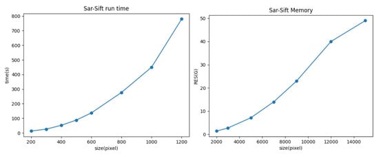
Figure 4.
Trends in time and space consumption along with the image size, with SAR-SIFT as the method.
Storage limitation is also one of the key considerations. In addition to this, the time complexity of the algorithm also needs to be taken seriously. This is because, in specific practical applications, most scenarios are expected to be processed in quasi-real time. It can be seen that, for small images, SAR-SIFT can be processed within seconds, and for medium-sized images, it takes roughly minutes. For larger images, although better registration results may be obtained, the program running time of several hours or even longer cannot be accepted. Parallel optimization processing was tried here, but it did not speed the process up significantly.
According to the above analysis, due to the special gradient calculation method and the storage requirements of the scale space, wide-swath SAR image processing will risk the boom of the time and space complexity. As a comparison, we also tried the method of combining ORB with GMS for large image processing, but the final solution turned out to be wrong. The above has shown the time and spatial complexity from a qualitative point of view. The following uses SIFT as an example to analyze the reasons for the high time complexity from a formula perspective. The SIFT algorithm mainly covers several stages, as shown in Figure 5.
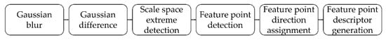
Figure 5.
The pipeline of the SIFT algorithm.
The overall time complexity is composed of the sum of the complexity for each stage. Assume that the size of the currently processed image is NxN.
- Regarding Gaussian blur, there are a total of groups of images, and each group consists of s scales; for the original-resolution image NxN, Gaussian filter group isThe corresponding time complexity is . For each pixel, a weighted sum of the surrounding Gaussian filtering is required, with complexity:The complexity of all of the groups is
- To calculate the Gaussian difference, subtract each pixel of adjacent scales once in one direction.
- To calculate the extremum detection in scale space, each point is compared with 26 adjacent points in the scale space. If the whole points are larger or smaller than the point, it is regarded as an extreme point; the complexity is
- For keypoint detection, the principal curvature needs to be calculated. The computational complexity of each point is , so the total time complexity of all of the groups is considering extrema and keypoints.
- For the keypoint orientation distribution, keypoint amplitude, and directionNon-keypoint points with magnitudes close to the peak are added as newly added keypoints. The total number of output points isThe computational complexity of each point is , and the total complexity is .
- For the feature point descriptor generation, the complexity of each point is , and the total complexity is .
Based on the analysis of the above results, we believe that the reasons for the failure of the above algorithm in actual wide-swath SAR image registration are as follows: (1) It is inefficient to calculate the scale space of the entire image. For most areas, it is not easy to find feature points that can establish a mapping relationship, which leads to potential ineffective calculations. Not only are these time-consuming, the corresponding scale space and feature points descriptor also consume a lot of storage resources. (2) For the feature point sets obtained from the two images, one-to-one matching needs to be carried out by the brute force calculation of the Euclidean distance, etc. Most points are not possible candidate points, and the calculated Euclidean distance needs to be stored, such that again there is an invalid calculation during the match.
From the perspective of the algorithm’s operation process, we will discuss the reason why algorithms such as SAR-SIFT are good at sub-image registration but fail in wide-swath images. The most obvious factors are time and space consumption. The reason can be found from a unified aspect: calculation and storage are not directional. There is redundancy in the calculation of the scale space. Some areas can be found beforehand in order to reduce the calculation range of the scale space, and the calculation amount of subsequent mismatch can also be reduced. At the same time, feature point matching does not have certain directivity because, for feature points in a small area, points from most of the area in another image are not potential matching ones. Therefore, redundant calculation and storage can be omitted.
In this paper, the idea of improving the practicality of wide-swath SAR image registration is to reduce the calculation range of the original image and the range of candidate points according to certain criteria. Based on the coarse registration results of the candidate regions, we determine the approximate spatial correspondences, and then perform more refined feature calculations and matching in the corresponding image slice regions.
In this work, the corresponding slice areas with a higher probability of feature points are selected. K-means++ is used to obtain the clustering centers of coarse matching points in the first step. The clustering center is marked as the geometric center in order to obtain the image slices. By using the geometric transformation relationship, a set of image pairs corresponding approximately to the same geographic locations are obtained. Adopting this approach has the following advantages:
- There are often more candidate regions of feature points near the cluster center.
- There is usually enough spatial distance between the clustering centers.
- The clustering center usually does not fall on the edge of the image.
K-means++ is an unsupervised learning method which is usually used in scenarios such as data mining. K-means++ needs to cluster N observation samples into K categories. Here, K = 4. the cluster centers are used as the slice geometric centers, and the slice size is set to 640 × 640. According to the above process, a series of rough matching image groups are obtained within an error of about ten pixels.
2.4. Dense Matching of the Sub-Image Slices
After the above processing is performed on the original-resolution SAR image, a set of SAR image slices are obtained. As is known, compared with optical image registration, an SAR image meets many difficulties: it has a low resolution and signal-to-noise ratio, overlay effects, perspective shrinkage, and a weak texture. Therefore, the original-resolution SAR image’s alignment is more difficult than the optical alignment.
This article uses Transformer. Based on the features extracted by CNN, Transformers are used to obtain the feature descriptors of the two images. The global receptive field provided by Transformer enables the method in this article to fuse the local features and contextual location information, which can produce dense matching in low-texture areas (usually, in low-texture areas, it is difficult for feature detectors to generate repeatable feature points).
The overall process consists of several steps, as shown in the lower half of Figure 2:
- The feature extraction network HRNet (High-Resolution Net) [41]: Before this step, we combine ORB and GMS to obtain the image rough matching results, use the K-means++ method to obtain the cluster centers of the rough matching feature points, and obtain several pairs of rough matching image pairs. The input of the HRNet is every rough matching image pair, and the output of the network is the high and low-resolution feature map after HRNet’s feature extraction and fusion.
- The low-resolution module: The input is a low-resolution feature map obtained from HRNet, which is expanded into a one-dimensional form and added with positional encoding. The one-dimensional feature vector after position encoding is processed by the Performer [42] to obtain the feature vector weighted by the global information of the image.
- The matching module: The one-dimensional feature vector obtained from the two images in the previous step is operated to obtain a similarity matrix. The confidence matrix is obtained after softmax processing on the similarity matrix. The pairs that are greater than a threshold in the confidence matrix and satisfy the mutual proximity criterion are selected as the rough matching prediction.
- Refine module: For each coarse match obtained by the matching module, a window of size wxw is cut from the corresponding position of the high-resolution feature map. The features contained in the window are weighted by the Performer, and the accurate matching coordinates are finally obtained through cross-correlation and softmax. For each pair of rough matching images, the outputs of the above step are matched point pairs with precise coordinates, and after the addition of the initial offset of rough matching, all of the point pairs are fused into a whole matched point set. After the implementation of the RANSAC filtering algorithm, the final overall matching point pair is generated, and then the spatial transformation solution is completed.
2.4.1. HRNet
Traditional methods such as VGGNet [43] and ResNets (Residual Networks) [44] include a series of convolution and pooling, which loses a lot of spatial detail information. The HRNet structure maintains high-resolution feature maps, and combines high- and low-resolution subnet structures in parallel to obtain multi-scale information.
HRNet is used as a network model for multi-resolution feature extraction in this method. At the beginning of this paper, we tried a variety of convolutional neural network models, including ResNets, EfficientNet [45] and FPN [46]; we found that HRNet has the best effect. The HRNet’s structure is shown in Figure 6; the network is composed of multiple branches, including the fusion layer with different resolution branches’ information interactions, and the transition layer, which is used to generate the 1/2 resolution downsampling branch. By observing the network input and output of HRNet at different stages, it can be seen that multi-resolution feature maps with multi-level information will be output after the full integration of the branches with different resolutions.
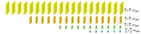
Figure 6.
HRNet architecture diagram.
The Transformer part of this paper requires high and low resolution to complete the coarse matching of the feature points and the more accurate positioning of specific areas. HRNet, as a good backbone, outputs feature maps with a variety of resolutions to choose from and full interaction between the feature maps, such that it contains high-level semantic information with a low resolution, and low-level detail information with a high resolution.
In addition, the subsequent part of this paper makes further attempts to combine different resolutions. It can be seen in subsequent chapters that improving the resolution of the feature maps in the rough matching stage can significantly increase the number of matching point pairs. Default HRNet outputs 1/2, 1/4, 1/8 resolution feature maps. Under the constraints of the experimental environment, we chose 1/5 and 1/2 as the low and high resolutions. The reason will be discussed in Section 3. Experimental Results and Analyses. The 1/5 resolution can be obtained from other resolutions by interpolation. The 1/2 resolution feature map cascades the 1 × 1 convolutional layer and the output works as the fine-level feature map. The 1/4 and 1/8 resolution feature maps are all interpolated to 1/5 resolution. After stitching, the coarse-level feature map is obtained through the 1 × 1 convolutional layer.
2.4.2. Performer
The Transformer has outstanding performance in many fields of CV, such as classification and detection. With the help of a multi-head self-attention mechanism, the Transformer can capture richer characteristic information. Generally speaking, Transformer complexity is squared with sequence length. In order to improve the speed of training and inference, a linear time complexity Transformer was also proposed recently, i.e., Performer [42]. It can achieve faster self-attention through the positive Orthogonal Random features approach.
Self-attention (as shown in Figure 7) performs an attention-weighted summation of the current data and global data, and realizes a special information aggregation by calculating the importance of the current location feature relative to other location features. The feedforward part contains the linear layer and the GELU (Gaussian Error Linear Unit) activation function. Each layer adopts Layer Normalization in order to ensure the consistency of the feature distribution, and to accelerate the convergence speed of the model training.
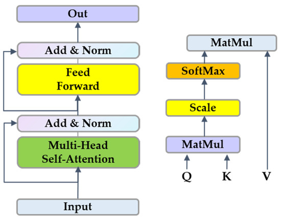
Figure 7.
Performer (Transformer) encoder architecture and self-attention schematic diagram.
As is shown in reference [42], Performer can achieve space complexity O(Lr + Ld + rd) and time complexity O(Lrd), but the original Transformer’s regular attention is O(L2 + Ld) and O(L2d), respectively. The sinusoidal position encoding formula used in this work is as follows:
Based on the features extracted by CNN, Performers are used to obtain the feature descriptors of the two images. The global receptive field provided by Performer enables our method to fuse local features and contextual location information, which can produce dense matching in low-texture areas (usually, in low-texture areas, it is difficult for feature detectors to generate repeatable feature points).
2.4.3. Training Dataset
Due to the influence of noise, it is difficult to accurately annotate the control points of an SAR image, and the corresponding matching dataset of an SAR image is not common. MegaDepth [47] contains 196 groups of different outdoor scenes; it applies SOTA (State-of-the-Art) methods to obtain depth maps, camera parameters, and other information. The dataset contains different perspectives and periodic scenes. Considering the dataset size and GPU memory, 1500 images were selected as a validation set, and the long side of the image was scaled to 640 during the training and 1200 during the verification.
2.4.4. Loss Function
As in [37], this article uses a similar loss function configuration. Here is a brief explanation. Pc is the confidence matrix returned by dual softmax. The true label of the confidence matrix is calculated by the camera parameters and depth maps. The nearest neighbors of the two sets of low-resolution grids are used as the true value of the coarse matching Mc, and the low resolution uses negative log-likelihood as the loss function.
The high resolution adopts the L2 norm. For a point, the uncertainty is measured by calculating the overall variance in the corresponding heatmap. The real position of the current point is calculated from the reference point, camera position, and depth map. The total loss is composed of low- and high-resolution items.
2.5. Merge and Solve
After obtaining the corresponding matching point sets of each image slice pair, the final solution requires mapping point sets of the entire image. Considering that the registration mapping geometric relationship solved by each set of slices is not necessarily the same, this work merges all of the point sets. The RANSAC method is used here to obtain the final result, i.e., a set of corresponding subsets describing the two large images. The corresponding point numbers must be less than the sum of the independent one. Without bells and whistles, the affine matrix of the entire image is solved.
3. Experimental Results and Analyses
In this section, we design several experiments to validate the performance of our methods from three perspectives: (1) the comparative performance tests with SOTA methods for different data sources, (2) the checkerboard visualization of the matching, (3) scale, rotation and noise robustness tests, and (4) the impact of the network’s high- and low-resolution settings on the results. First, a brief introduction to the experimental datasets is given.
3.1. Experimental Data and Settings
In this work, datasets from five sources were used to verify the algorithm’s effectiveness, which contains GF-3, TerraSAR-X, Sentinel-1, ALOS, and SeaSat. These data include a variety of resolutions, polarization modes, orbital directions, and different terrains. Table 1 and Figure 8 contain detailed information. DEC and ASC mean “descending” and “ascending”, respectively.

Table 1.
Experimental datasets.
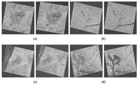
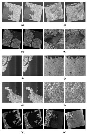
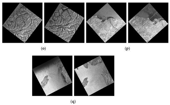
Figure 8.
The SAR image datasets (a–q) of datasets 1–17.
In order to verify the effectiveness of the proposed matching method, several evaluation criteria were used to evaluate the accuracy of the SAR image registration, as shown below:
- The root mean square error, RMSE, is calculated by the following formula:
- NCM stands for the number of matching feature point pairs filtered by the RANSAC algorithm, mainly representing the number of feature point pairs participating in the calculation of the spatial transformation model. It is a filtered point subset of the matching point pairs output by algorithms such as SAR-SIFT. For the solution of the affine matrix, the larger the value, the better the image registration effect.
3.2. Performance Comparison
In this section, we compare the proposed method with several methods: SAR-SIFT, HardNet [48], TFeat [49], SOSNet [50], LoFTR, KAZE-SAR, and CMM-Net. HardNet, TFeat, and SOSNet use GFTT [51] as the feature point detector, and the patch size of the above methods is 32 × 32. GFTT will pick the top N strongest corners as feature points. The comparison methods are introduced briefly as follows:
- SAR-SIFT uses SAR-Harris space instead of DOG to find the key points. Unlike the square descriptor of SIFT, SAR-SIFT uses the circular descriptor to describe neighborhood information.
- HardNet proposes the loss that maximizes the nearest negative and positive examples’ interval in a single batch. It uses the loss in metric learning, and outputs feature descriptors with 128 dimensionalities, like SIFT.
- SOSNet adds second-order similarity regularization for local descriptor learning. Intuitively, first-order similarity aims to give descriptors of matching pairs a smaller Euclidean distance than descriptors of non-matching pairs. The second-order similarity can describe more structural information; as a regular term, it helps to improve the matching effect.
- TFeat uses triplets to learn local CNN feature representations. Compared with paired sample training, triplets containing both positive and negative samples can generate better descriptors and improve the training speed.
- LoFTR proposes coarse matching and refining dense matches by a self-attention mechanism. It combines high- and low-resolution feature maps extracted by CNN to determine rough matching and precise matching positions, respectively.
- KAZE-SAR uses a nonlinear diffusion filter to build the scale space.
- CMM-Net uses VGGNet to extract high-dimensional feature maps and build descriptors. It uses triplet margin ranking loss to balance the universality and uniqueness of the feature points.
As for our method, we set K = 4 and window size = 640 for the sub-image. SAR-SIFT and KAZE-SAR are traditional methods, and Hardnet, Tfeat, SOSNet, LoFTR, and CMM-Net are deep learning methods. The algorithm in this paper was trained and tested on a server with a GPU of NVIDIA TITAN_X (12GB), a CPU of Intel(R) Core(TM) I7-5930K @3.50GHZ, and a memory size of 128 GB. The comparison experiment was carried out using the same hardware. As will be discussed later (Section 3.4), under existing hardware conditions, (1/2,1/5) resolution was adopted in this paper in order to achieve the best effect, and was used as the final network model to calculate the speed and accuracy of the algorithm. Like diverse methods, in addition to feature point detection and feature point description, other processing steps are consistent with our method, including the rough matching of sub-sampling images and the acquisition of subimages. The other settings were based on the original settings of the algorithm in order to ensure the fairness of the comparison.
Table 2 shows the performance results of several methods on the above dataset, in which the best performance corresponding to each indicator is shown in bold. ‘-’ in the table means that the matching result of the corresponding algorithm is incorrect. It can be seen that the performance of our method on RMSE is better than the comparison methods in more than half of the datasets. For all of the SAR image registration datasets, the performance of our method reaches the sub-pixel level. Considering NCM, our method obtains the best performance for all of the total datasets, as well as a better spatial distribution of points, i.e., dense matching. Figure 9 shows that our method’s NCMs are higher than those of other methods, while the RMSEs are lower in most cases.
Table 2.
RMSE and NCM of diverse methods on the datasets.
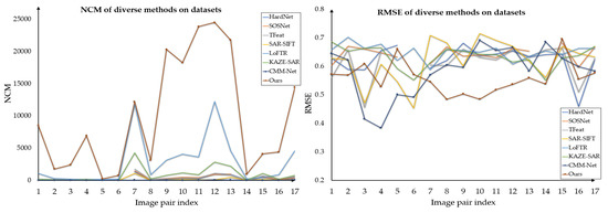
Figure 9.
NCM and RMSE of diverse methods on the datasets.
3.3. Visualization Results
In order to display the matching accuracy more intuitively, we added the checkerboard mosaic images. In Figure 10, the continuity of the lines can reflect the matching accuracy. As the pictures show, the areas and lines overlap well, indicating the high accuracy of the proposed method.
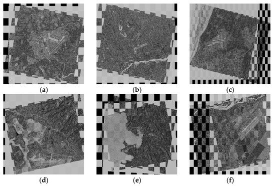
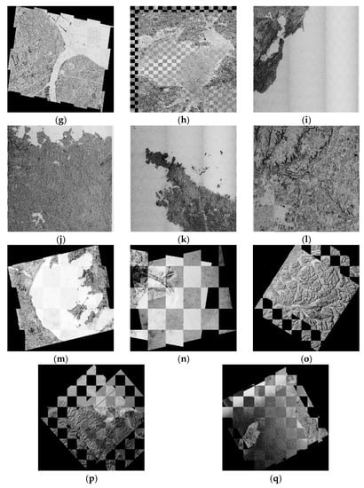
Figure 10.
The checkerboard mosaic images (a–q) of datasets 1–17.
Considering that our method adopts the strategy of fusing local and global features, it can fully extract matching point pairs in the selected local area, which leads to better solutions that are closer to the affine transformation relationship of real images. In the data pairs 14 and 17, the two images have relatively strong changes in their radiation intensities, and the method in this paper can still achieve good matching results, which proves that the method has certain robustness to changes in radiation intensity. Dataset 5 contains two images of different orbit directions. It can be seen from the road and other areas in the figure that the matching is precise. Datasets 2 and 7 contain multi-temporal images of different polarizations. Due to the scattering mechanism, the same objects in different polarizations may be different in the images. Our method demonstrates the stability in multi-polarization.
3.4. Analysis of the Performance under Different Resolution Settings
Considering that our proposed method has a coarse-to-fine step, we analyzed the registration performance of different resolution settings to find the best ratio. In this experiment, we tested several different high and low resolutions. Table 3 shows the corresponding performances, respectively, and the method of the best performance for each data is indicated in bold. All of the resolution parameter combinations include (1/4, 1/16), (1/2,1/8), (1,1/8), and (1/2,1/5).
Table 3.
RMSE and NCM of the different resolution settings on the datasets.
It can be seen from Table 3 that, for the datasets, the resolution of (1/2,1/5) has the best performance. It is shown in Table 3 that the size of the low resolution directly affects the overall matched point’s number. It can be found intuitively that the total potential points of resolution 1/16 are a quarter of 1/8′s point number (1/2 × 1/2 = 1/4). As such, configuration (1/2,1/5) can obtain more matched point pairs. Take configurations (1/2,1/8) and (1,1/8) for an example; for high-resolution feature maps, the number of matched points increases to a certain extent with the increase of the resolution. However, here, the GPU memory requested by configuration (1,1/5) exceeds the upper limit of the machine used in this work, so we chose a compromise configuration, (1/2,1/5).
4. Discussion
The experimental results corroborate the accuracy and robustness of our method. There are three main reasons for this: First, the features extracted based on Transorfmer are richer, including the local gray information of the image itself, and global information such as the context. Second, the down-sampled image has stronger semantic information, and is suitable for traditional registration methods. The subsequent registration is provided with a better initial result of coarse matching. Third, according to the K-means++ clustering method, the relationship between the original image and the sub-images to be registered is constructed, and representative sub-images are obtained in order to reduce time and space consumption.
From the performance analysis and model hyperparameter comparison experiments, it can be seen that our proposed method achieved stable and accurate matching results under different ground object scenes and various sensors’ data conditions. Now, we will further examine the rotation, scaling and noise robustness of the proposed method. Furthermore, another vital criterion—the execution time—needs to be compared. Finally, we will show the matching accuracy’s impact on downstream tasks.
4.1. Rotation and Scale Test
In practical applications, there are often resolution inconsistencies and rotations between the sensed image and the reference image. In order to test the rotation and scale robustness of the proposed subimage registration method, we experimented on the data with a simulated variation. The RADARSAT SAR sensor collected the data of Ottawa, in May and August 1997, respectively. The size of the two original images is 350 × 290, as shown in Figure 11.
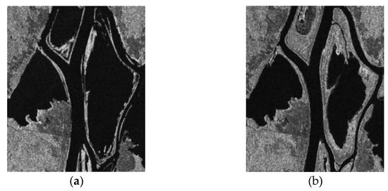
Figure 11.
The Ottawa data: (a) May 1997 and (b) August 1997.
A matching test between the two images at 5° intervals from –15° to 15° was carried out to verify the rotation robustness. In addition, two scaling ratios of 0.8 and 1.2 were tested to simulate the stability of the image registration algorithm at different resolutions. In all of the above cases, more than 100 matching points could be extracted between the two SAR images with an RMSE of around 0.7 (the subpixel level). As Figure 12 and Figure 13 show, the proposed method has rotation and scale robustness.
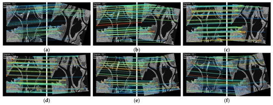
Figure 12.
The registration performance of SAR images at varying rotations: (a) –15°, (b) –10°, (c) –5°, (d) 5°, (e) 10°, and (f) 15°.
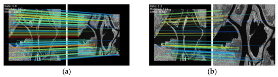
Figure 13.
The registration performance of SAR images at varying sizes: (a) 0.8, and (b)1.2.
In addition, we can see that, under different rotation and scaling conditions, a large number of matching points can be obtained not only in the strong edge area but also in the weak texture area. This is significantly helpful for SAR image registration including low-texture areas. The simulation experiments reflect the validity of image registration with various changes in real scenes.
4.2. Robustness Test of the Algorithm to Noise
Previously, we discussed the robustness of the algorithm to scale and rotation. Considering that there is often a high degree of noise in SAR images, taking motion error as an example, SAR images in practical applications will possess some unfocused positions. Whether or not it has stable performance in noisy scenes, this paper refers to the method and results of [52]; here, two sets of images—before and after autofocus—are tested in order to verify the stability of the algorithm.
Here, we used our sub-image method to register the defocusing data; the results can be seen in Figure 14, and although the image data has a high degree of noise due to error motion defocusing, our method can still obtain a good matching result between two images, and matching points can also be maintained at a high level with error at the subpixel level. It is thus proven that the proposed method is robust to noise.
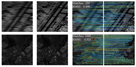
Figure 14.
Algorithm robustness test in a noise scenario.
4.3. Program Execution Time Comparison
In actual tasks, the registration process needs to achieve real-time or quasi-real-time analysis; as such, in addition to the accuracy of the algorithm, timeliness is also a focus of measurement. We also compared several representative methods on a selection of characteristic dataset pairs, i.e., 2, 8, 12, 17. The algorithm in this paper selected the resolution configuration of (1/2, 1/5) as a comparison. As Table 4 shows, our method is significantly faster than the traditional method, SAR-SIFT, and slightly slower than other deep learning methods.
Table 4.
Execution time (s) comparison of the different methods.
Methods like TFeat use a shallow convolutional neural network so that the feature extraction phase is faster. Given that our approach is multi-stage, the model is relatively complex. Except for the model itself, our method obtains the most matching points and consumes exponentially more time in both the feature point matching and filtering stages. Although the running time is slightly longer, the SAR image registration performance is significantly improved. In further work, we will consider improving the efficiency by adjusting the distillation learning of the feature extraction module in order to obtain a lightweight network with similar performance.
4.4. Change Detection Application
In some applications—such as SAR image change detection—the simultaneous analysis of SAR images with different acquisition conditions is inevitable. We carried out a simple analysis, and the registration result was applied to the task of SAR image change detection. In this project, we use the previously mentioned Ottawa dataset.
In this experiment, we rotate one of the images to achieve a relative image offset. The Ottawa data of two SAR images were matched first, and the change detection results were obtained after they were processed by two registration methods: SAR-SIFT and ours. The PCA-Kmeans [53] method was used as the basic change detection method. Kappa was used as the change detection performance metric; the formula is as follows:
The Kappa coefficient can be used to measure classification accuracy. The higher the value is, the more accurate the classification result is. Compared with SAR-SIFT, our proposed method improved the kappa indicator from 0.307 to 0.677, which shows that accurate registration can lead to better change detection results. Intuitively, from Figure 15, we can see that our method results (b) are more similar to the ground truth (c) than SAR-SIFT (a). The deviation of the image registration will cause different objects to be mistaken for the same area during change detection, which will be mistaken for obvious changes.
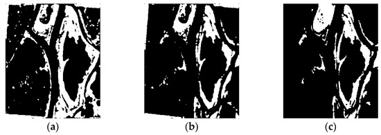
Figure 15.
The change map: (a) SAR-SIFT, (b) the proposed method, and (c) the ground truth.
5. Conclusions
This paper proposes a novel wide-swath SAR image registration method which uses a combination of traditional methods and deep learning to achieve accurate registration. Specifically, we combined the clustering methods and traditional registration methods to complete the stable extraction of representative sub-image slices containing high-probability regions of feature points. Inspired by Performer’s self-attention mechanism, a coarse-to-fine sub-image dense-matching method was adopted for the SAR image matching under different terrain conditions, including weak texture areas.
The experimental results demonstrate that our method achieved good performance for different datasets which include multi-temporal, multi-polarization, multi-orbit direction, rotation, scaling, noise changes. At the same time, the combination of CNN and Performer verified the effectiveness of the strong representation in SAR image registration. Under the framework of sub-images matching to original images matching, stable dense matching can be obtained in high-probability regions. This framework overcomes the time-consuming problem of the traditional method of matching. Compared with existing methods, more matching point pairs can be obtained by adjusting the model parameter settings in our method. Rotation, scaling and noise experiments were also carried out to verify the robustness of the algorithm. The results showed that a large number of matching point pairs can be obtained even in regions with weak textures, which shows that our method can combine local and global features to characterize feature points more effectively.
In addition, the experimental results suggest that the running time is significantly less than those of traditional methods but slightly longer than those of similar deep learning methods; as such, the way in which to further simplify the network model will be the focus of the next step. Meanwhile, the matching between heterogeneous images is also a topic that can be discussed further.
Author Contributions
Conceptualization, Y.F., H.W. and F.W.; validation, Y.F., H.W. and F.W.; formal analysis, Y.F., H.W. and F.W.; investigation, Y.F., H.W. and F.W.; resources, Y.F., H.W. and F.W.; data curation, Y.F., H.W. and F.W.; writing—original draft preparation, Y.F., H.W. and F.W.; writing—review and editing, Y.F., H.W. and F.W.; visualization, Y.F., H.W. and F.W.; funding acquisition, Y.F., H.W. and F.W. All authors have read and agreed to the published version of the manuscript.
Funding
This work was supported in part by the National Natural Science Foundation of China (Grant No. 61901122), the Natural Science Foundation of Shanghai (Grant No. 20ZR1406300, 22ZR1406700), and the China High-resolution Earth Observation System (CHEOS)-Aerial Observation System Project (30-H30C01-9004-19/21).
Institutional Review Board Statement
Not applicable.
Informed Consent Statement
Not applicable.
Data Availability Statement
Data sharing not applicable.
Conflicts of Interest
The authors declare no conflict of interest.
References
- Kulkarni, S.C.; Rege, P.P. Pixel level fusion techniques for SAR and optical images: A review. Inf. Fusion 2020, 59, 13–29. [Google Scholar] [CrossRef]
- Song, S.L.; Jin, K.; Zuo, B.; Yang, J. A novel change detection method combined with registration for SAR images. Remote Sens. Lett. 2019, 10, 669–678. [Google Scholar] [CrossRef]
- Tapete, D.; Cigna, F. Detection of Archaeological Looting from Space: Methods, Achievements and Challenges. Remote Sens. 2019, 11, 2389. [Google Scholar] [CrossRef] [Green Version]
- Suri, S.; Schwind, P.; Reinartz, P.; Uhl, J. Combining mutual information and scale invariant feature transform for fast and robust multisensor SAR image registration. In Proceedings of the American Society of Photogrammetry and Remote Sensing (ASPRS) Annual Conference, Baltimore, MD, USA, 9–13 March 2009. [Google Scholar]
- Stone, H.S.; Orchard, M.T.; Chang, E.; Martucci, S.A.; Member, S. A Fast Direct Fourier-Based Algorithm for Sub-pixel Registration of Images. IEEE Trans. Geosci. Remote Sens. 2001, 39, 2235–2243. [Google Scholar] [CrossRef] [Green Version]
- Xiang, Y.; Wang, F.; You, H. An Automatic and Novel SAR Image Registration Algorithm: A Case Study of the Chinese GF-3 Satellite. Sensors 2018, 18, 672. [Google Scholar] [CrossRef] [Green Version]
- Pallotta, L.; Giunta, G.; Clemente, C. Subpixel SAR image registration through parabolic interpolation of the 2-D cross correlation. IEEE Trans. Geosci. Remote Sens. 2020, 58, 4132–4144. [Google Scholar] [CrossRef] [Green Version]
- Lowe, D.G. Distinctive image features from scale-invariant keypoints. Int. J. Comput. Vis. 2004, 60, 91–110. [Google Scholar] [CrossRef]
- Yan, K.; Sukthankar, R. PCA-SIFT: A more distinctive representation for local image descriptors. In Proceedings of the 2004 IEEE Computer Society Conference on Computer Vision and Pattern Recognition, CVPR 2004, Washington, DC, USA, 27 June–2 July 2004; Volume 2, pp. 506–513. [Google Scholar]
- Dellinger, F.; Delon, J.; Gousseau, Y.; Michel, J.; Tupin, F. SAR-SIFT: A SIFT-like algorithm for SAR images. IEEE Trans. Geosci. Remote Sens. 2014, 53, 453–466. [Google Scholar] [CrossRef] [Green Version]
- Pourfard, M.; Hosseinian, T.; Saeidi, R.; Motamedi, S.A.; Abdollahifard, M.J.; Mansoori, R.; Safabakhsh, R. KAZE-SAR: SAR Image Registration Using KAZE Detector and Modified SURF Descriptor for Tackling Speckle Noise. IEEE Trans. Geosci. Remote Sens. 2021, 60, 5207612. [Google Scholar] [CrossRef]
- Alcantarilla, P.F.; Bartoli, A.; Davison, A.J. KAZE features. In Proceedings of the European Conference on Computer Vision, Florence, Italy, 7–13 October 2012; Springer: Berlin, Germany, 2012; pp. 214–227. [Google Scholar]
- Xiang, Y.; Jiao, N.; Wang, F.; You, H. A Robust Two-Stage Registration Algorithm for Large Optical and SAR Images. IEEE Trans. Geosci. Remote Sens. 2021, in press. [Google Scholar] [CrossRef]
- LeCun, Y.; Bengio, Y.; Hinton, G. Deep learning. Nature 2015, 521, 436–444. [Google Scholar] [CrossRef]
- Chen, S.; Wang, H.; Xu, F.; Jin, Y.Q. Target Classification using the Deep Convolutional Networks for SAR Images. IEEE Trans. Geosci. Remote Sens. 2016, 54, 4806–4817. [Google Scholar] [CrossRef]
- Hou, X.; Ao, W.; Song, Q.; Lai, J.; Wang, H.; Xu, F. FUSAR-Ship: Building a high-resolution SAR-AIS matchup dataset of Gaofen-3 for ship detection and recognition. Sci. China Inf. Sci. 2020, 63, 140303. [Google Scholar] [CrossRef] [Green Version]
- Wang, S.; Quan, D.; Liang, X.; Ning, M.; Guo, Y.; Jiao, L. A deep learning framework for remote sensing image registration. ISPRS J. Photogramm. Remote Sens. 2018, 145, 148–164. [Google Scholar] [CrossRef]
- Geng, J.; Ma, X.; Zhou, X.; Wang, H. Saliency-Guided Deep Neural Networks for SAR Image Change Detection. IEEE Trans. Geosci. Remote Sens. 2019, 57, 7365–7377. [Google Scholar] [CrossRef]
- He, H.; Chen, M.; Chen, T.; Li, D. Matching of remote sensing images with complex background variations via Siamese convolutional neural network. Remote Sens. 2018, 10, 355. [Google Scholar] [CrossRef] [Green Version]
- Zheng, Y.; Sui, X.; Jiang, Y.; Che, T.; Zhang, S.; Yang, J.; Li, H. SymReg-GAN: Symmetric Image Registration with Generative Adversarial Networks. IEEE Trans. Pattern Anal. Mach. Intell. 2021, in press. [Google Scholar] [CrossRef]
- Li, Z.; Zhang, H.; Huang, Y. A Rotation-Invariant Optical and SAR Image Registration Algorithm Based on Deep and Gaussian Features. Remote Sens. 2021, 13, 2628. [Google Scholar] [CrossRef]
- Mao, S.; Yang, J.; Gou, S.; Jiao, L.; Xiong, T.; Xiong, L. Multi-Scale Fused SAR Image Registration Based on Deep Forest. Remote Sens. 2021, 13, 2227. [Google Scholar] [CrossRef]
- Luo, X.; Lai, G.; Wang, X.; Jin, Y.; He, X.; Xu, W.; Hou, W. UAV Remote Sensing Image Automatic Registration Based on Deep Residual Features. Remote Sens. 2021, 13, 3605. [Google Scholar] [CrossRef]
- Lan, C.; Lu, W.; Yu, J.; Xu, Q. Deep learning algorithm for feature matching of cross modality remote sensing images. Acta Geodaetica et Cartographica Sinica. 2021, 50, 189. [Google Scholar]
- Rublee, E.; Rabaud, V.; Konolige, K.; Bradski, G.R. ORB: An efficient alternative to SIFT or SURF. In Proceedings of the IEEE International Conference on Computer Vision (ICCV), Barcelona, Spain, 6–13 November 2011; pp. 2564–2571. [Google Scholar]
- Bian, J.; Lin, W.Y.; Matsushita, Y.; Yeung, S.K.; Nguyen, T.D.; Cheng, M.M. Gms: Grid-based motion statistics for fast, ultra-robust feature correspondence. In Proceedings of the IEEE Conference on Computer Vision and Pattern Recognition (CVPR), Honolulu, HI, USA, 25–30 June 2017; pp. 4181–4190. [Google Scholar]
- Arthur, D.; Vassilvitskii, S. K-means++: The Advantages of Careful Seeding. In Proceedings of the Eighteenth Annual ACM-SIAM Symposium on Discrete Algorithms, New Orleans, LA, USA, 7–9 January 2007; Society for Industrial and Applied Mathematics: Philadelphia, PA, USA; pp. 1027–1035. [Google Scholar]
- Fischler, M.A.; Bolles, R.C. Random sample consensus—A paradigm for model-fitting with applications to image-analysis and automated cartography. Commun. ACM 1981, 24, 381–395. [Google Scholar] [CrossRef]
- Krizhevsky, A.; Sutskever, I.; Hinton, G.E. ImageNet Classification with Deep Convolutional Neural Networks. In Advances in Neural Information Processing Systems 25; Pereira, F., Burges, C.J.C., Bottou, L., Weinberger, K.Q., Eds.; Curran Associates, Inc.: Red Hook, NY, USA, 2012; pp. 1097–1105. [Google Scholar]
- Zhang, Z.; Wang, H.; Xu, F.; Jin, Y.Q. Complex-valued convolutional neural network and its application in polarimetric SAR image classification. IEEE Trans. Geosci. Remote Sens. 2017, 55, 7177–7188. [Google Scholar] [CrossRef]
- Guo, Q.; Wang, H.; Xu, F. Scattering Enhanced attention pyramid network for aircraft detection in SAR images. IEEE Trans. Geosci. Remote Sens. 2020, 99, 1–18. [Google Scholar] [CrossRef]
- Duan, Y.; Liu, F.; Jiao, L.; Zhao, P.; Zhang, L. SAR Image segmentation based on convolutional-wavelet neural network and markov random field. Pattern Recognit. 2016, 64, 255–267. [Google Scholar] [CrossRef]
- Vaswani, A.; Shazeer, N.; Parmar, N.; Uszkoreit, J.; Jones, L.; Gomez, A.N.; Kaiser, Ł.; Polosukhin, I. Attention is all you need. In Advances in Neural Information Processing Systems; MIT Press: Cambridge, MA, USA, 2017; pp. 5998–6008. [Google Scholar]
- Wang, Z.; Zhao, J.; Zhang, R.; Li, Z.; Lin, Q.; Wang, X. UATNet: U-Shape Attention-Based Transformer Net for Meteorological Satellite Cloud Recognition. Remote Sens. 2022, 14, 104. [Google Scholar] [CrossRef]
- Zhao, C.; Wang, J.; Su, N.; Yan, Y.; Xing, X. Low Contrast Infrared Target Detection Method Based on Residual Thermal Backbone Network and Weighting Loss Function. Remote Sens. 2022, 14, 177. [Google Scholar] [CrossRef]
- Xu, X.; Feng, Z.; Cao, C.; Li, M.; Wu, J.; Wu, Z.; Shang, Y.; Ye, S. An Improved Swin Transformer-Based Model for Remote Sensing Object Detection and Instance Segmentation. Remote Sens. 2021, 13, 4779. [Google Scholar] [CrossRef]
- Sun, J.; Shen, Z.; Wang, Y.; Bao, H.; Zhou, X. LoFTR: Detector-free local feature matching with transformers. In Proceedings of the IEEE/CVF Conference on Computer Vision and Pattern Recognition, Montreal, QC, Canada, 11–17 October 2021; pp. 8922–8931. [Google Scholar]
- Bay, H.; Tuytelaars, T.; Van Gool, L. SURF: Speeded Up Robust Features. In Proceedings of the 9th European Conference on Computer Vision, Graz, Austria, 7–13 May 2006; pp. 404–417. [Google Scholar]
- Rosten, E.; Drummond, T. Machine learning for high-speed corner detection. In Proceedings of the 9th European Conference on Computer Vision, Graz, Austria, 7–13 May 2006; pp. 430–443. [Google Scholar]
- Calonder, M.; Lepetit, V.; Strecha, C.; Fua, P. BRIEF: Binary Robust Independent Elementary Features. In Proceedings of the 11th European Conference on Computer Vision, Heraklion, Greece, 5–11 September 2010; pp. 778–792. [Google Scholar]
- Sun, K.; Xiao, B.; Liu, D.; Wang, J. Deep high-resolution representation learning for human pose estimation. In Proceedings of the IEEE Conference on Computer Vision and Pattern Recognition, Long Beach, CA, USA, 16–20 June 2019; pp. 5693–5703. [Google Scholar]
- Choromanski, K.; Likhosherstov, V.; Dohan, D.; Song, X.; Gane, A.; Sarlos, T.; Weller, A. Rethinking attention with performers. In Proceedings of the International Conference on Learning Representations, Virtual, 26 April–1 May 2020. [Google Scholar]
- Simonyan, K.; Zisserman, A. Very deep convolutional networks for large-scale image recognition. In Proceedings of the International Conference on Learning Representations, Banff, AB, Canada, 14–16 April 2014. [Google Scholar]
- He, K.; Zhang, X.; Ren, S.; Sun, J. Deep Residual Learning for Image Recognition. In Proceedings of the 2016 IEEE Conference on Computer Vision and Pattern Recognition (CVPR), Las Vegas, NV, USA, 27–30 June 2016; pp. 770–778. [Google Scholar]
- Tan, M.; Le, Q. Efficientnet: Rethinking model scaling for convolutional neural networks. In Proceedings of the International Conference on Machine Learning, Long Beach, CA, USA, 9–15 June 2019; pp. 6105–6114. [Google Scholar]
- Lin, T.Y.; Dollar, P.; Girshick, R.; He, K.; Hariharan, B.; Belongie, S. Feature Pyramid Networks for Object Detection. In Proceedings of the 2017 IEEE Conference on Computer Vision and Pattern Recognition (CVPR), Honolulu, HI, USA, 21 July–26 July 2017; IEEE Computer Society: Washington, DC, USA, 2017. [Google Scholar]
- Li, Z.; Snavely, N. MegaDepth: Learning Single-View Depth Prediction from Internet Photos. In Proceedings of the 2018 IEEE/CVF Conference on Computer Vision and Pattern Recognition (CVPR), Salt Lake City, UT, USA, 18–23 June 2018; pp. 2041–2050. [Google Scholar]
- Mishchuk, A.; Mishkin, D.; Radenovic, F.; Matas, J. Working hard to know your neighbor’s margins: Local descriptor learning loss. In Advances in Neural Information Processing Systems; MIT Press: Cambridge, MA, USA, 2017; pp. 4826–4837. [Google Scholar]
- Balntas, V.; Riba, E.; Ponsa, D.; Mikolajczyk, K. Learning Local Feature Descriptors with Triplets and Shallow Convolutional Neural Networks. In Proceedings of the British Machine Vision Association (BMVC) 2016, York, UK, 19–22 September 2016; Volume 1, p. 3. [Google Scholar]
- Tian, Y.; Yu, X.; Fan, B.; Wu, F.; Heijnen, H.; Balntas, V. SOSNet: Second Order Similarity Regularization for Local Descriptor Learning. In Proceedings of the Computer Vision and Pattern Recognition, Long Beach, CA, USA, 16–20 June 2019; pp. 11008–11017. [Google Scholar]
- Shi, J.; Tomasi, C. Good features to track. In Proceedings of the 1994 Proceedings of IEEE Conference on Computer Vision and Pattern Recognition, Seattle, WA, USA, 21–23 June 1994; pp. 593–600. [Google Scholar]
- Pu, W. SAE-Net: A Deep Neural Network for SAR Autofocus. IEEE Trans. Geosci. Remote Sens. 2022, in press. [Google Scholar] [CrossRef]
- Celik, T. Unsupervised change detection in satellite images using principal component analysis and k-means clustering. IEEE Geosci. Remote Sens. Lett. 2009, 6, 772–776. [Google Scholar] [CrossRef]
Publisher’s Note: MDPI stays neutral with regard to jurisdictional claims in published maps and institutional affiliations. |
© 2022 by the authors. Licensee MDPI, Basel, Switzerland. This article is an open access article distributed under the terms and conditions of the Creative Commons Attribution (CC BY) license (https://creativecommons.org/licenses/by/4.0/).