Abstract
The volatility of the cumulative displacement of landslides is related to the influence of external factors. To improve the prediction of nonlinear changes in landslide displacement caused by external influences, a new combined forecasting model of landslide displacement has been proposed. Variational modal decomposition (VMD) was used to obtain the trend and fluctuation sequences of the original sequence of landslide displacement. First, we established a stacked long short time memory (LSTM) network model and introduced rainfall and reservoir water levels as influencing factors to predict the fluctuation sequence; next, we used a threshold autoregressive (TAR) model to predict the trend sequence, following which the trend and fluctuation prediction sequence were superimposed to obtain the cumulative predicted displacement of the landslide. Finally, the VMD-stacked LSTM-TAR combination model based on the variational modal decomposition, stacked long short time memory network, and a threshold autoregressive model was built. Taking the landslide of Baishuihe in the Three Gorges Reservoir area as an example, through comparison with the prediction results of the VMD-recurrent neural network-TAR, VMD-back propagation neural network-TAR, and VMD-LSTM-TAR, the proposed combined prediction model was noted to have high accuracy, and it provided a novel approach for the prediction of volatile landslide displacement.
1. Introduction
There are many landslide disasters, wide coverage areas, and frequent activities globally which cause serious economic losses and casualties every year. Currently, global navigation satellite system (GNSS) deformation monitoring is used to monitor absolute displacement of the landslide surface [1,2]. The displacement monitoring data is an important basis for the early warning of landslide disasters through tolerance judgment and imminent slip model analysis [3,4]. Mining effective information from long-term monitoring data, extracting the relationship between landslide surface displacement changes and influencing factors, and then analyzing and predicting landslide deformation is of great significance for the early warning of landslide disasters [5,6,7].
The cumulative displacement of the landslide in the Three Gorges Reservoir area shows a step-like development, which may be the result of the influence of seasonal rainfall and reservoir water level fluctuations. In addition to a linear natural change trend, the cumulative displacement of landslides also has a sharp increase. This seasonal change, which may be caused by changes in rainfall and reservoir water levels, is difficult to predict. It is studied as a fluctuating displacement with a seasonal cycle. The landslide displacement affected by external factors is generally decomposed in a time series, and the natural development trend displacement of the landslide body and the fluctuating displacement caused by external environmental factors can be predicted [8,9]. Currently, the methods for decomposing the cumulative displacement of landslides include the moving average [10], exponential smoothing [11], empirical mode decomposition [12], and collective empirical mode decomposition methods [13]. Conventional decomposition methods require decomposition of modeling samples, which reduces the subsequent training data. The variational mode decomposition (VMD) method can decompose the cumulative landslide displacement as a signal in the frequency domain and alleviate the modal aliasing problem in the common empirical mode decomposition method [14,15,16]. For the fluctuation displacement series after separating the overall trend, the statistical machine learning models were normally used, such as the back propagation neural network (BPNN) [17] and extreme machine learning [18]; however, they are all static network models, and their ability to process changes in a time series is weak. Hochreiter et al. [19] improved recurrent neural networks (RNN) and proposed long short time memory (LSTM), which solved the problem of gradient explosion or disappearance [20,21], allowing for the processing of long-term sequence data. By stacking multiple layers of LSTM, the effect of the memory unit on the LSTM model is enhanced and the long-term sequence prediction ability of the model is improved [22,23]. The polynomial model prediction results of the traditional trend item prediction method are limited by the model, and the fitting results are unstable. An improved method based on the autoregressive (AR) model has been proposed. The threshold autoregressive (TAR) model [24,25] predicts the trend item of the cumulative landslide displacement, segmented by threshold, and improves the trend prediction ability through threshold segmentation.
The landslides in the Three Gorges Reservoir area are affected by environmental factors. In addition to rainfall, there are also reservoir water levels. By focusing on landslides affected by rainfall and reservoir water levels in this study, a combined prediction method of cumulative landslide displacement based on VMD, stacked LSTM network models, and TAR models was proposed, taking the Baishuihe landslide as an example. In Zigui County in the Three Gorges Reservoir Area, using the time series decomposition method based on VMD to decompose the cumulative landslide displacement, we built a stacked LSTM network and introduced rainfall and reservoir water level influencing factors to establish a prediction model for the cumulative displacement fluctuation term of the landslide. In addition, the TAR model was used to predict the trend item, and the validity of the combined VMD-LSTM-TAR landslide displacement prediction model was demonstrated through the model prediction accuracy verification and by comparison with other models.
2. Theory and method
2.1. Variational Modal Decomposition
VMD is an adaptive modal variational method [26,27] that can separate various frequency components in the signal data. Because the cumulative displacement of a landslide has a certain periodic volatility, the VMD method is used to decompose the cumulative displacement of the landslide, and the obtained components are divided and superimposed according to the frequency to obtain the trend and fluctuation items of the cumulative landslide displacement.
The main steps of VMD are as follows:
- (1)
- Calculate the analytical signal of each mode using the transform to obtain the unilateral spectrum, alias it with the corresponding center frequency, modulate the baseband of the spectrum, and estimate the bandwidth of each mode. The restricted variational expression is:where are the k-th modal component and its center frequency after decomposition, respectively, represents the partial derivative, j represents the imaginary unit, is the Dirac function, * represents convolution, s.t. represents the constraint, represents the original time series to be decomposed, and K is the number of modal decompositions.
- (2)
- Introduce the secondary penalty factor and the Lagrangian multiplication operator to transform the constrained variational formula into an unconstrained problem:
- (3)
- Use the alternating direction multiplication operator to continuously update each modal component and the corresponding center frequency , extend the saddle point of the Lagrangian expression, and optimize the iterative expression:where are the Fourier transforms of , respectively, and is the noise tolerance. When Formula (6) is satisfied, the iteration is completed, and are the outputs.where is the convergence tolerance.
The quadratic penalty factor and number k of modal decomposition can be obtained by the constraint optimization of (7):
where is the original cumulative displacement and is the decomposition component.
2.2. Stacked Long Short Time Memory Network Model
The LSTM network model solves the problem of gradient disappearance in gradient backpropagation [28,29], learns continuous tasks, and resets internal states.
The LSTM unit uses input, forget, and output gates to update the learning and memory of the time-series data [30,31]. The LSTM unit structure is shown in Figure 1.
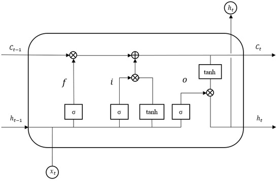
Figure 1.
LSTM unit structure. represent memory unit, output vector, input vector, forget gate, input gate, and output gate, respectively, and represent the bitwise addition and multiplication operations, represents the sigmoid activation function, and tanh represents the hyperbolic tangent function.
The LSTM unit can be defined by the following functions:
Status of each gate control unit:
Memory unit status update:
where represent the forget, input, and output gates, respectively, represent the weight matrix and bias vector of the network, respectively, and represent the input memory state, current memory state, final output vector, and input vector, respectively. represents the sigmoid activation function, represents the hyperbolic tangent function, and represents the multiplication of the corresponding elements.
Increasing the depth of the LSTM layer can improve the performance of the entire prediction model and reveal more complex features in the data. For a large amount of complex data, a recursive network with multiple hidden layers has better learning and prediction performance than a shallow surface network [32]. The stacking of LSTM levels has a greater effect than the increase in the internal memory units in the LSTM unit. The neural network model is formed by coupling multiple LSTM layers [33,34,35], and the prediction performance is improved when there are long-term related data or multivariate time datasets. Therefore, this study adopted the stacked LSTM architecture to learn and train the monthly rainfall and average reservoir water level datasets and predict the displacement of fluctuation items. As shown in Figure 2, enters layer LSTM 1 with the hidden state as the input vector, and outputs as the input of layer LSTM 2. After all the LSTM layers have been stacked, the final output, is obtained.
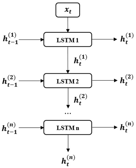
Figure 2.
Stacked LSTM layers.
2.3. Threshold Autoregressive Model
The threshold Auto Regressive (TAR) model is an improvement of the autoregressive (AR) model. Due to the segmentation of the threshold, the model can model the data sequence in segments, which can avoid the accumulation of modeling errors caused by long-term series data. Through parameter optimization, a prediction model that best fits the curve change can be established, which can describe the change of the sequence in detail. This study uses this model to conduct modeling prediction experiments on the trend displacement obtained by time series decomposition.
The AR model is a method used to analyze the internal correlation of data [36,37]. For observation sequence , we define the p-order autoregressive model AR(p) as follows:
where is not 0, is the autoregressive coefficient sequence and is the zero-mean white noise sequence.
The TAR model is a segmented AR model, which introduces m − 1 thresholds in the value range of the observation sequence ; the entire time series is divided into m threshold intervals, in which can be used to represent the upper and lower bounds, respectively, according to the number of delay steps, the number of threshold delay steps here refers to the number of samples in each segment modeling interval, and the values are allocated to different threshold intervals. Then, AR models of different orders are used for the intervals in the interval. The model is:
where is the coefficient vector of the k-th threshold interval segmented model, is the order of the AR model used in the k-th threshold interval, is the number of delay steps in the AR model, is the number of threshold intervals, is the threshold value, and is a mutually independent normal white noise sequence.
The model optimizes and finds the most suitable multidimensional parameters for the observed sample sequence. The optimization method sets the maximum threshold delay to when selecting the threshold value. For any , can be used. The delay value is divided into m groups, and each group builds an AR model and calculates the Akaike Information Criterion (AIC) value. The AIC criterion is a standard for measuring the goodness of fit of a statistical model. When the sum of m AIC values is the smallest, it corresponds to parameters being optimal. The formula for calculating AIC value is as follows:
In the formula, are the number of samples, variance of the sample residuals, and order of the AR model in the k-th threshold interval, respectively.
3. VMD-Stacked LSTM-TAR Combined Prediction Model
The combined VMD-stacked LSTM-TAR prediction model proposed in this study processes and predicts data based on the VMD method, the stacked LSTM network model, and the TAR model. The main steps of the combined model data prediction are as follows:
- (1)
- The VMD method is used to decompose the global positioning system (GPS) landslide monitoring surface displacement data to obtain the displacement series of different frequencies. The high-frequency and low-frequency components are combined to obtain the fluctuation and trend series.
- (2)
- A stacked LSTM network model was established, and rainfall and reservoir water level data were introduced to dynamically predict the change in the fluctuation displacement sequence. The data input set includes the rainfall of the previous month, the rainfall of the current month, the fluctuation displacement of the previous month, the average reservoir water level of the previous month, and the average reservoir water level of the current month; the output data comprise the forecast data for the fluctuation displacement of the current month.
- (3)
- A TAR model is established to dynamically predict the trend sequence changes and summarize the time series superimposition to obtain the cumulative displacement prediction value of the landslide.
The data processing steps are shown in Figure 3.
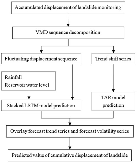
Figure 3.
Data processing steps of the combined prediction model.
The accuracy evaluation indicators of the cumulative landslide displacement prediction model are the mean absolute error (MAE), root mean square error (RMSE), mean relative error (MRE), and goodness of fit , and the formulas are as follows:
where are the original observation and model prediction values of the landslide displacement, respectively, is the mean of the original value, and is the number of prediction periods.
4. Engineering Application and Model Verification
Taking the Baishuihe landslide in Zigui County of the Three Gorges Reservoir Area as an example, the landslide body is located in the wide valley section of the Yangtze River, the geographical location as shown in Figure 4, with a monoclinic bedding slope, which is high in the south and low in the north, and spreads out to the Yangtze River in a stepped shape. The Baishuihe landslide is 500 m long from north to south, 430 m wide from east to west, with an area of 21.5 × 10⁴ m2, an average thickness of about 30 m, a volume of 645 × 104 m3, and the main sliding direction is 20°. It is a large bedding soil landslide. The landslide mass is mainly composed of Quaternary residual slope accumulated gravel soil, and the landslide bedrock lithology is medium-thick sandstone with thin mudstone. The sliding zone is mainly composed of silty clay containing gravel or breccia, and the rock and soil material components of some sliding zones are breccia and clay. Atotal of 11 GPS monitoring points [38] were placed in the Baishuihe landslide body, and the monitoring data of monitoring point ZG118 on the middle and lower parts of landslide body and the monitoring point ZG93 on the northeastern part of landslide body were selected for model prediction and verification. The monitoring data of ZG118 were collected monthly from January 2006 to December 2012, a total of 72 periods of GPS surface displacement observation data; the monitoring data of ZG93 were collected from January 2006 to December 2011, a total of 60 periods of GPS surface displacement observation data. The data changes are shown in Figure 5. The rainfall intensity will change seasonally, and the cumulative displacement of the landslide will also rise periodically. When the rainfall increases, the cumulative displacement of the landslide will also rise at the same time node, the uplift of the cumulative displacement of landslides often occurs when the monthly average reservoir water level is low. This study uses the trends of rainfall intensity changes and average reservoir water level changes to predict the occurrence of landslide cumulative displacement fluctuations.
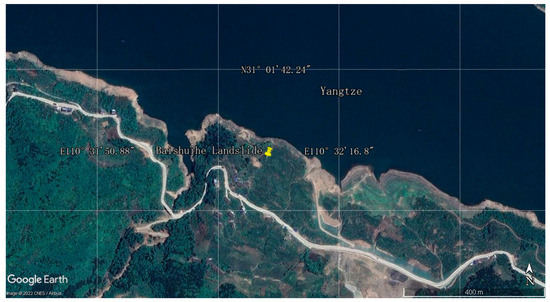
Figure 4.
The geographical location figure in Google Earth (yellow tag is the landslide body).
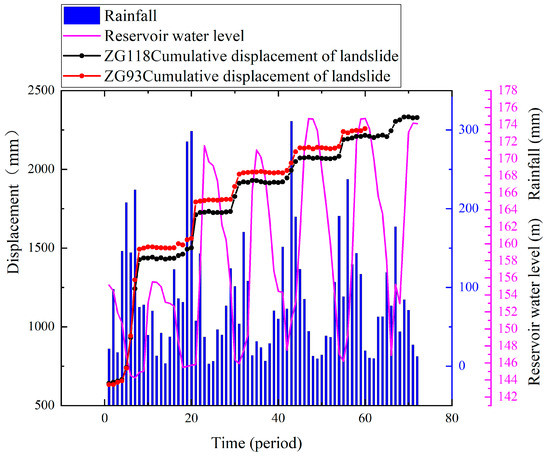
Figure 5.
Landslide monitoring data. Time series of landslide monitoring data, among which the ZG118 monitoring point displacement data has a total of 70 periods, the ZG93 monitoring point has a total of 60 periods, and the rainfall is the regional rainfall, with a total of 72 periods, and the reservoir water level is the water level in the area adjacent to the landslide body, with a total of 72 periods.
4.1. Model Verification Experiment Example 1
Experimental example 1 shows the data of monitoring point ZG118. The experimental steps are as follows.
VMD is used to decompose the horizontal displacement sequence of the GPS monitoring points. The parameter selection is based on Formula (7), the convergence tolerance is set to , the secondary penalty factor is set to 0.5, the number k of the modal decomposition is set to 10, and 10 modal components are obtained. The time sequence and frequency spectrum diagrams of the decomposition are shown in Figure 6.
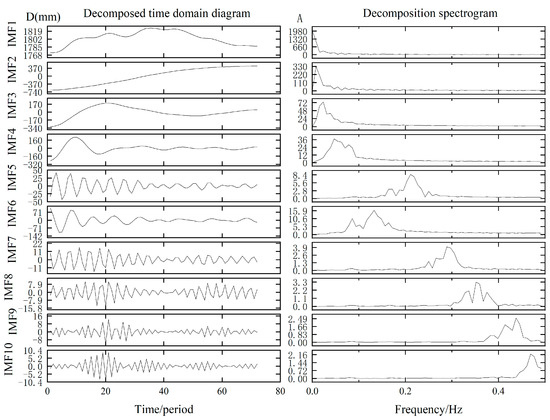
Figure 6.
VMD decomposition results. D (left) represents the displacement signal, and A (right) represents the amplitude of change.
As shown in Figure 6, the two components with frequencies close to zero in the decomposition spectrum have the smallest periodic fluctuations. The trend sequence is obtained by the IMF1-2 combination, and the fluctuation sequence is obtained by the remaining IMF combination. The time-series decomposition results of the original cumulative landslide displacement are shown in Figure 7.
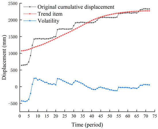
Figure 7.
Extracted values of trend and volatility items.
For the 72 periods of landslide displacement data, periods 1–48 were used as training samples, and periods 49–72 were used as prediction test values. A stacked LSTM network model was established. The model uses three LSTM layers, and the number of neurons in each layer is obtained through K-fold cross-validation optimization, which are 16, 4, and 16, respectively. The model prediction introduces multiple influencing factors. The rainfall of the previous month, the rainfall of the current month, the fluctuation displacement of the previous month, the average reservoir water level of the previous month, and the average reservoir water level of the current month were used as input data, and the fluctuation displacement of the current month was the output forecast data.
The stacked RNN, BPNN, and LSTM models were established to verify the prediction effect of the combined prediction model. Compared with the stacked LSTM model constructed in this study, the combined model proposed in this study and the model used for comparison use its optimal prediction results, that is, each model has undergone K-fold cross-validation parameter optimization and multiple iterations. After obtaining the optimal parameters and initial weights, the prediction effect is compared. In order to ensure uniformity, the K-fold cross-validation method is used to optimize network parameters for all models, and initial weights are determined through multiple iterations, and the optimal prediction results of each model are compared. The prediction results of the volatility items are shown in Figure 8. The predicted value of the stacked LSTM model has the highest degree of fit with the extracted value of the fluctuation displacement, and the overall prediction value was relatively stable. There are fewer errors in the prediction. In comparison, the BPNN model fluctuates in the prediction results as the number of periods increases, and large errors occur after the displacement increases, whereas the stacked LSTM model has a relatively stable prediction accuracy over time, and the stacked RNN model has a poor prediction effect as the number of periods increases, indicating the superiority of the LSTM structure to the improved RNN.
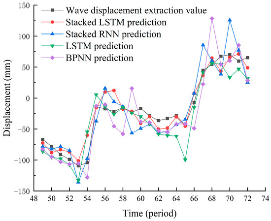
Figure 8.
Forecast results of volatility items.
In addition, a TAR prediction model was established to dynamically model and predict the cumulative displacement trend item of the landslide. The modeling sample and test sets were the same as the prediction of the cumulative displacement fluctuation item. The parameters of the model were set as follows: the maximum AR order was 5, the number of threshold intervals was two, the maximum threshold delay was set to 5, the default minimum AIC value was 1 × 10¹⁰, 30–70% of the sample, and the quantile interval searched for the optimal threshold with a progress of 1%. The prediction results for the trend item are shown in Figure 9. The RMSE of the prediction result was 0.1742 mm, the MAE was 0.3261 mm, and the R2 was 0.9999.
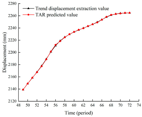
Figure 9.
Forecast results of trend items.
The time series of the trend item prediction sequence and the fluctuation item prediction sequence were superimposed to obtain the cumulative displacement prediction value of the landslide. To verify the prediction accuracy of the combined VMD-stacked LSTM-TAR model, VMD-RNN-TAR, VMD-BPNN-TAR, and VMD were also established using the prediction effects of the LSTM-TAR model, and the VMD-stacked LSTM-TAR model has the highest prediction accuracy. The prediction results of each model are shown in Figure 10, and the accuracy evaluation indicators are listed in Table 1.
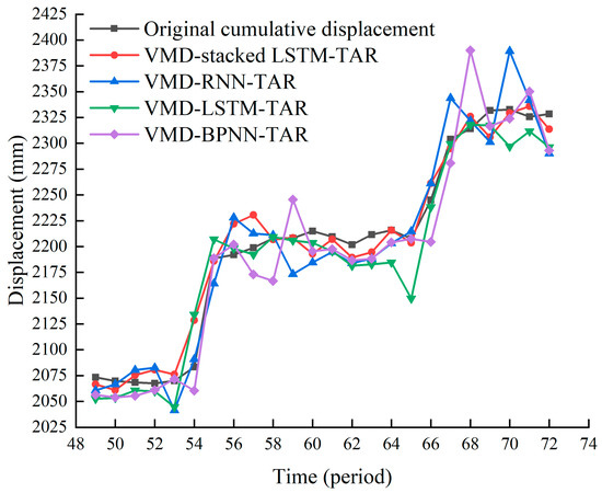
Figure 10.
Curves of prediction results of various models.

Table 1.
Accuracy evaluation of each model.
From Table 1, the combined VMD-stacked LSTM-TAR prediction model has the highest prediction accuracy, with MAE of 12.5969 mm, RMSE of 16.8010 mm, MRE of 0.0057, and the prediction accuracy index is better than the VMD-RNN-TAR, VMD-BPNN-TAR, and VMD-LSTM-TAR prediction results. The R2 of the VMD-stacked LSTM-TAR prediction result was 0.9648, and the predicted value had a good correlation with the original value. As shown in Figure 10, the VMD-stacked LSTM-TAR model has fewer sharp points in the prediction value, the stacking of LSTM levels has a greater effect than the increase in the internal memory unit of the LSTM, and the prediction of the cumulative landslide displacement is more stable, which confirms the predictive ability and reliability of the constructed model.
4.2. Model Verification Experiment Example 2
Experimental example 2 shows the data of monitoring point ZG93. The experimental steps are as follows.
VMD is used to decompose the horizontal displacement sequence of the GPS monitoring points. The parameter selection is based on Formula (7), the convergence tolerance is set to , the secondary penalty factor is 0.6, the modal decomposition number k is 10, and ten modal components are obtained. The decomposed sequence and spectrum diagrams are shown in Figure 11.
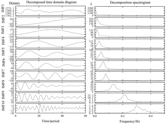
Figure 11.
VMD decomposition results. D (left) represents the displacement signal, and A (right) represents the amplitude of change.
As shown in Figure 11, the two components with frequencies close to zero in the decomposed spectrum have the smallest periodic fluctuations. The trend sequence is obtained by the IMF1-2 combination, and the fluctuation sequence is obtained by the remaining IMF combination. The time-series decomposition results of the original cumulative landslide displacement are shown in Figure 12.
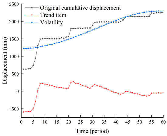
Figure 12.
Extracted value of trend and volatility items.
For the 60 periods of landslide displacement data, periods 1–48 were used as training samples, and periods 49–60 were used as prediction test values. A stacked LSTM network model was established. The model uses three LSTM layers, and the number of neurons in the three layers, obtained through K-fold cross-validation optimization, is as follows: 16, 3, and 16. The rainfall, fluctuation displacement, average reservoir water level of the previous month, and the rainfall, average reservoir water level of the current month are used as input data, and the fluctuation displacement of the current month is the output forecast data.
The stacked RNN, BPNN, and LSTM models were established to verify the prediction effect of the combined prediction model. The prediction results of the volatility items for each model are shown in Figure 13. The stacked LSTM model predictive value has the highest degree of fit for the fluctuation displacement, and the error is smaller than that of the other models; the BPNN and LSTM models show greater error fluctuations in the prediction results as the number of prediction periods increases; the overall prediction effect of the stacked RNN model is poor, and there are many spikes during the prediction. When all models predict the second half of the period, the prediction error increases, which may be caused by the weaker correlation between the changes in data and the influencing factors. The ability to map from changes in rainfall and reservoir water levels to changes in displacement is weakened, and the prediction effect deteriorates.
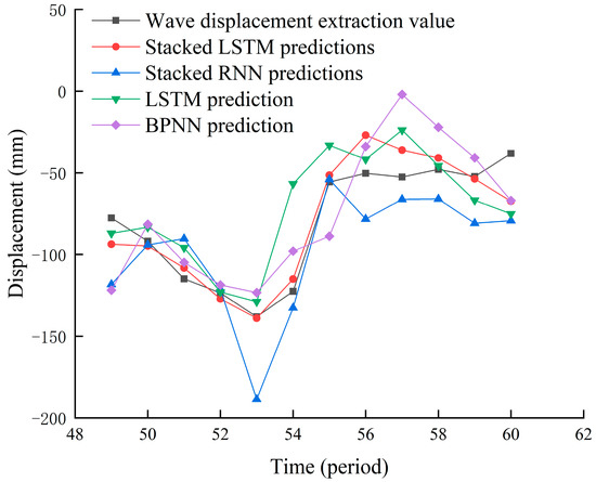
Figure 13.
Forecast results of volatility items.
In addition, a TAR prediction model was established to dynamically model and predict the cumulative displacement trend item of the landslide. The modeling sample and test sets were the same as the prediction of the cumulative displacement fluctuation item. The parameters of the model are set as follows: the maximum AR order is 5, the number of threshold intervals is two, the maximum threshold delay is 5, the default minimum AIC value is 1 × 10¹⁰, and the search for optimal thresholds is 1% of the 30–70% positioning range. The prediction results for the trend item are shown in Figure 14. The RMSE of the prediction was 0.9248 mm, while the MAE was 0.7126 mm and the R2 was 0.9988.
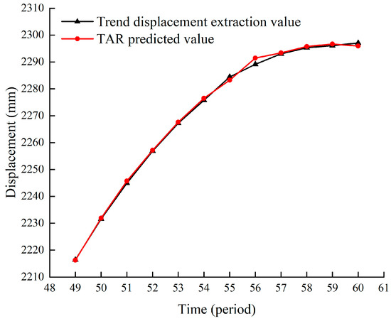
Figure 14.
Forecast results of trend items.
The time series of the trend and fluctuation item prediction sequences were superimposed to obtain the cumulative displacement prediction value of the landslide. To verify the prediction accuracy of the built VMD-stacked LSTM-TAR combination model, VMD-RNN-TAR, VMD-BPNN-TAR, and VMD were also established using the prediction effects of the LSTM-TAR model. The VMD-stacked LSTM-TAR model had the highest prediction accuracy. The prediction results of each model are shown in Figure 15, and the accuracy evaluation indicators are listed in Table 2.
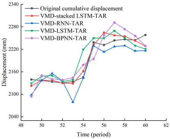
Figure 15.
Curves of prediction results of various models.

Table 2.
Accuracy evaluation of each model.
As shown in Table 2, the VMD-stacked LSTM-TAR combined prediction model has the highest prediction accuracy: MAE is 11.3149 mm, RMSE is 15.4577 mm, MRE is 0.0051, and the prediction accuracy index is better than the prediction results of VMD-RNN-TAR, VMD-BPNN-TAR, and VMD-LSTM-TAR. The R2 of the VMD-stacked LSTM-TAR prediction result was 0.9183, and the predicted value had a strong correlation with the original value. As shown in Figure 15, the prediction value of the VMD-stacked LSTM-TAR model is the most consistent with the original displacement change. In the first half of the prediction, the VMD-stacked LSTM-TAR had the highest prediction accuracy and the most stable prediction of the cumulative landslide displacement. The learning effect of the affected factors was not good in the second half of the prediction. Because VMD-stacked LSTM-TAR is based on LSTM, it still has a good prediction effect, and the prediction results are better than those of VMD-RNN-TAR and VMD-BPNN-TAR, which confirms the prediction ability and reliability of the constructed model.
5. Discussion
This study uses the data of the ZG118 and ZG93 monitoring points of the Baishuihe landslide in Zigui County of the Three Gorges Reservoir area to verify the combined prediction model. The landslide is located in the reservoir area. In addition to the geological conditions of the landslide body, it is also affected by changes in rainfall and reservoir water level. This study proposes a new combined prediction method to discuss the nonlinear effects of rainfall and reservoir water level changes on the cumulative displacement of the landslide. At the same time, the accuracy of the proposed model is verified, and a data analysis method is provided for the monitoring and early warning of landslides in the reservoir area.
In this study, VMD is used as the extraction method of the fluctuation displacement and trend displacement of the landslide, and the signal decomposition of the landslide displacement is carried out in the frequency domain. After the decomposition, the changing frequency of each displacement signal component can be clearly observed. When the components are combined, the selection is clearer and can accurately separate the trend term and the fluctuation term of the cumulative displacement of the landslide.
In the prediction experiment of the trend item, the TAR model is used to predict and verify the accuracy of the trend item displacement of the ZG118 and ZG93 monitoring points, and the R2 can reach 0.99, indicating that the predicted displacement is consistent with the actual displacement. The forecasting accuracy is high, meeting the demand for trend forecasting.
The prediction error of the cumulative displacement of the landslide mainly comes from the fluctuation term. After the statistical analysis of the prediction verification results, in the ZG118 monitoring point data model prediction experiment, VMD-stacked LSTM-TAR is relatively better than VMD-RNN-TAR, VMD-LSTM-TAR, and VMD-BPNN-TAR; the prediction accuracy MAE is increased by 39.70%, 31.08%, 39.13%, and the prediction accuracy RMSE is increased by 32.06%, 28.38%, 36.25%, respectively. In the ZG93 monitoring point data model prediction experiment, compared with VMD-RNN-TAR, VMD-LSTM-TAR, VMD-BPNN-TAR, and the prediction accuracy MAE of VMD-stacked LSTM-TAR is improved by 47.19%, 41.70%, and 55.30%, respectively;. The prediction accuracy RMSE is improved by 42.77%, 43.21%, and 46.94%, respectively. It can be seen that the stacked LSTM method has a greater improvement in the prediction accuracy of the fluctuation term. On the one hand, the LSTM model has the stronger ability to mine time series data. On the other hand, the stacked LSTM layer improves the prediction accuracy and stability of the LSTM model. The increase in the depth of the LSTM structure enhances the ability of deep learning on complex data, not just before and after memory updates on the time series.
The research object is the landslide in the Three Gorges Reservoir area, and the external environmental factors are rainfall and the change of the reservoir water level. In this study, the sample data are the rainfall of the previous month, the rainfall of the current month, the average reservoir water level of the previous month, the average reservoir water level of the current month, and the fluctuation displacement of the previous month, and they are used to predict the displacement of the current month and to explore the effect of monthly rainfall and reservoir water level changes on monthly displacement. The combined prediction model based on the machine learning model was used to verify this prediction method. The experimental results show that this method can effectively predict the monthly variation of landslide displacement and has a higher prediction accuracy. Based on the displacement of the previous month, after a month of rainfall and changes in reservoir water levels, one can compare whether the predicted displacement this month is significantly different from the actual displacement change. If the difference is large, in addition to the influence of normal seasonal rainfall and reservoir water level fluctuations, the actual displacement of the landslide mass increases and there is a landslide acceleration. At this time, the monitoring sampling rate can be increased to support landslide warning with more data. Based on the prediction model, through long-term series learning and mining, the prediction accuracy can be improved, which can support the monitoring, analysis and early warning of landslides.
6. Conclusions
In this study, a VMD-stacked LSTM-TAR cumulative landslide displacement prediction model was constructed based on VMD, the stacked LSTM model, and the TAR model, and the cumulative landslide displacement was decomposed and reconstructed into the trend and seasonal fluctuation sequences under the landslide geological environment via the VMD method. We analyzed the impact of the location of monitoring points, as well as rainfall and reservoir water level changes, on the landslide displacement and introduced the rainfall of the previous and current months, the average reservoir water level of the previous month and current months, and the fluctuation displacement of the previous month to predict the fluctuation displacement of the month. We then established a multi-factor stacked LSTM model. By comparing the prediction results with other models, the stacked LSTM model was found to have better stability in predicting the fluctuation displacement. The prediction accuracy was higher than that of the LSTM model, and it was also affected by prediction interference. Our proposed model can consistently achieve the long-term prediction of LSTM. Moreover, the AR model was improved to establish the TAR model and predict the trend sequence of the cumulative landslide displacement. Finally, the trend and fluctuation sequences were combined to obtain the cumulative displacement of the landslide prediction. The prediction result is better than that of the combined model using LSTM, stacked RNN, and BPNN as the volatility prediction method. The prediction accuracy is the highest for the proposed model, which proves the effectiveness of the method proposed in this study for predicting landslides.
Using time series analysis and prediction, the prediction of the cumulative land-slide displacement is primarily aimed at the prediction of displacement fluctuation items affected by the environment. The establishing of a more effective and universal volatility displacement prediction model, the improvement of the ability of the model to assimilate landslide impact factors and landslide deformation, and to improve the prediction accuracy of the cumulative landslide displacement is of great significance for long-term safety monitoring and the early warning of landslides.
Author Contributions
Conceptualization, X.C. and R.T.; methodology, X.C.; software, X.C.; validation, Y.G., G.C. and T.L.; formal analysis, X.C., D.X.; investigation, Y.G.; resources, R.T.; data curation, R.T.; writing—original draft preparation, X.C.; writing—review and editing, Y.G. and R.T.; supervision, Y.G.; project administration, Y.G.; funding acquisition, R.T., Y.G. All authors have read and agreed to the published version of the manuscript.
Funding
This work was supported by the program of National Natural Science Foundation of China (Grant No: 41974032), the Applied Basic Research Project of Science and Technology Department of Sichuan Province, China (Grant No: 2020YJ0362), Science and Technology Open Fund of Sichuan Society of Surveying, Mapping and Geoinformatics (Grant No: CCX202114).
Institutional Review Board Statement
Not applicable.
Informed Consent Statement
Not applicable.
Data Availability Statement
Not applicable.
Acknowledgments
The authors thank the National Glacier and Permafrost Desert Science Data Center of China (http://www.ncdc.ac.cn, accessed on 10 January 2022) for data support. The authors thank the reviewers for their beneficial comments and suggestions.
Conflicts of Interest
The authors declare that they have no known competing financial interests or personal relationships that could have appeared to influence the work reported in this paper.
References
- Zarate, B.A.; Hamdouni, R.E.; Fernandez, T. GNSS and RPAS Integration Techniques for Studying Landslide Dynamics: Application to the Areas of Victoria and Colinas Lojanas, (Loja, Ecuador). Remote Sens. 2021, 13, 3496. [Google Scholar] [CrossRef]
- Segina, E.; Peternel, T.; Urbancic, T.; Realini, E.; Zupan, M.; Jez, J.; Caldera, S.; Gatti, A.; Tagliaferro, G.; Consoli, A.; et al. Monitoring Surface Displacement of a Deep-Seated Landslide by a Low-Cost and near Real-Time GNSS System. Remote Sens. 2020, 12, 3375. [Google Scholar] [CrossRef]
- Dong, M.; Wu, H.Y.; Hu, H.; Azzam, R.; Zhang, L.; Zheng, Z.R.; Gong, X.N. Deformation Prediction of Unstable Slopes Based on Real-Time Monitoring and DeepAR Model. Sensors 2021, 21, 14. [Google Scholar] [CrossRef] [PubMed]
- Wang, J.; Nie, G.G.; Gao, S.J.; Wu, S.G.; Li, H.Y.; Ren, X.B. Landslide Deformation Prediction Based on a GNSS Time Series Analysis and Recurrent Neural Network Model. Remote Sens. 2021, 13, 1055. [Google Scholar] [CrossRef]
- Frattini, P.; Crosta, G.B.; Rossini, M.; Allievi, J. Activity and kinematic behaviour of deep-seated landslides from PS-InSAR displacement rate measurements. Landslides 2018, 15, 1053–1070. [Google Scholar] [CrossRef]
- Calvello, M.; Piciullo, L. Assessing the performance of regional landslide early warning models: The EDuMaP method. Nat. Hazards Earth Syst. Sci. 2016, 16, 103–122. [Google Scholar] [CrossRef]
- Lazzari, M.; Piccarreta, M.; Ray, L.R.; Manfreda, S. Modeling Antecedent Soil Moisture to Constrain Rainfall Thresholds for Shallow Landslides Occurrence. Landslides-Investig. Monit. 2020, 5, 1–32. [Google Scholar] [CrossRef]
- Piegari, E.; Di Maio, R.; Avella, A. Recurrence time distribution and temporal clustering properties of a cellular automaton modelling landslide events. Nonlinear Processes Geophys. 2013, 20, 1071–1078. [Google Scholar] [CrossRef]
- Phengsuwan, J.; Shah, T.; James, P.; Thakker, D.; Barr, S.; Ranjan, R. Ontology-based discovery of time-series data sources for landslide early warning system. Computing 2020, 102, 745–763. [Google Scholar] [CrossRef]
- Merigo, J.M.; Yager, R.R. Aggregation operators with moving averages. Soft Comput. 2019, 23, 10601–10615. [Google Scholar] [CrossRef]
- Huang, F.M.; Yin, K.L.; Yang, B.B.; Li, X.; Liu, L.; Fu, X.L.; Liu, X.W. Landslide step displacement prediction based on time series decomposition and multivariate chaotic model. Earth Sci. 2018, 43, 887–898. [Google Scholar]
- Ghezaiel, W.; Ben Slimane, A.; Ben Braiek, E. Nonlinear multi-scale decomposition by EMD for Co-Channel speaker identification. Multimed. Tools Appl. 2017, 76, 20973–20988. [Google Scholar] [CrossRef]
- Niu, X.X.; Ma, J.W.; Wang, Y.K.; Zhang, J.R.; Chen, H.J.; Tang, H.M. A Novel Decomposition-Ensemble Learning Model Based on Ensemble Empirical Mode Decomposition and Recurrent Neural Network for Landslide Displacement Prediction. Appl. Sci. 2021, 11, 4684. [Google Scholar] [CrossRef]
- Seo, Y.; Kim, S.; Singh, V.P. Machine Learning Models Coupled with Variational Mode Decomposition: A New Approach for Modeling Daily Rainfall-Runoff. Atmosphers 2018, 9, 251. [Google Scholar] [CrossRef]
- Khan, M.S.; Hassan, S.A. Hydrological peaks evaluation at chitral and tarbela stations, Pakistan, using combined Bayesian regularized neural network and signal difference average based variational mode decomposition method: A case study. Water Supply 2022, 22, 1375–1387. [Google Scholar] [CrossRef]
- Kumar, A.; Zhou, Y.Q.; Xiang, J.W. Optimization of VMD using kernel-based mutual information for the extraction of weak features to detect bearing defects. Measurement 2020, 168, 108402. [Google Scholar] [CrossRef]
- Chen, H.Q.; Zeng, Z.G. Deformation Prediction of Landslide Based on Improved Back-propagation Neural Network. Cogn. Comput. 2013, 5, 56–62. [Google Scholar] [CrossRef]
- Shihabudheen, K.V.; Peethambaran, B. Landslide displacement prediction technique using improved neuro-fuzzy system. Arab. J. Geosci. 2017, 10, 502. [Google Scholar] [CrossRef]
- Hochreiter, S.; Schmidhuber, J. Long short-term memory. Neural Comput. 1997, 9, 1735–1780. [Google Scholar] [CrossRef]
- Sherstinsky, A. Fundamentals of Recurrent Neural Network (RNN) and Long Short-Term Memory (LSTM) network. Phys. D-Nonlinear Phenom. 2020, 404, 132306. [Google Scholar] [CrossRef]
- Vlachas, P.R.; Byeon, W.; Wan, Z.Y.; Sapsis, T.P.; Koumoutsakos, P. Data-driven forecasting of high-dimensional chaotic systems with long short-term memory networks. Proc. R. Soc. A-Math. Phys. Eengineering Sci. 2018, 474, 20170844. [Google Scholar] [CrossRef] [PubMed]
- Sebt, M.V.; Ghasemi, S.H.; Mehrkian, S.S. Predicting the number of customer transactions using stacked LSTM recurrent neural networks. Soc. Netw. Anal. Min. 2021, 11, 86. [Google Scholar] [CrossRef]
- Ravikumar, K.N.; Yadav, A.; Kumar, H.; Gangadharan, K.V.; Narasimhadhan, A.V. Gearbox fault diagnosis based on Multi-Scale deep residual learning and stacked LSTM model. Measurement 2021, 186, 110099. [Google Scholar] [CrossRef]
- Khan, M.Y.; Mittnik, S. Nonlinear time series modeling and forecasting the seismic data of the Hindu Kush region. J. Seismol. 2018, 22, 353–376. [Google Scholar] [CrossRef]
- Mir, A.; Ye, M.Q.; Imtiaz, H. Estimating the Effects of Free Trade Agreements on Imports, Exports and Trade Volume Using “Threshold Auto Regressive Model” (A Case Study of Pakistan). Am. J. Econ. 2018, 8, 113–122. [Google Scholar]
- Lu, X.S.; Miao, F.S.; Xie, X.X.; Li, D.Y.; Xie, Y.H. A new method for displacement prediction of “step-like” landslides based on VMD-FOA-SVR model. Environ. Earth Sci. 2021, 80, 542. [Google Scholar] [CrossRef]
- Miao, F.S.; Xie, X.X.; Wu, Y.P.; Zhao, F.C. Data Mining and Deep Learning for Predicting the Displacement of “Step-like” Landslides. Sensors 2022, 22, 481. [Google Scholar] [CrossRef] [PubMed]
- Li, L.M.; Guo, F.; Wen, Z.Z.; Chen, P.N.; Zhang, S.F. Dynamic prediction of landslide displacement based on long and short-term memory and multiple influence factors. Sci. Technol. Eng. 2020, 20, 13559–13567. [Google Scholar]
- Fischer, T.; Krauss, C. Deep learning with long short-term memory networks for financial market predictions. Eur. J. Oper. Res. 2018, 270, 654–669. [Google Scholar] [CrossRef]
- Wang, J.; Jiang, W.P.; Li, Z.; Lu, Y. A New Multi-Scale Sliding Window LSTM Framework (MSSW-LSTM): A Case Study for GNSS Time-Series Prediction. Remote Sens. 2021, 13, 3328. [Google Scholar] [CrossRef]
- Wang, F.; Chen, Y.N.; Li, Z.; Fang, G.H.; Li, Y.P.; Wang, X.X.; Zhang, X.Q.; Kayumba, P.M. Developing a Long Short-Term Memory (LSTM)-Based Model for Reconstructing Terrestrial Water Storage Variations from 1982 to 2016 in the Tarim River Basin, Northwest China. Remote Sens. 2021, 13, 889. [Google Scholar] [CrossRef]
- Ballesteros, M.; Dyer, C.; Goldberg, Y.; Smith, N.A. Greedy Transition-Based Dependency Parsing with Stack LSTMs. Comput. Linguist. 2017, 43, 311–347. [Google Scholar] [CrossRef]
- Zhao, M.C.; Yao, X.J.; Wang, J.; Yan, Y.; Gao, X.; Fan, Y.N. Single-Channel Blind Source Separation of Spatial Aliasing Signal Based on Stacked-LSTM. Sensors 2021, 21, 4844. [Google Scholar] [CrossRef] [PubMed]
- Kouchak, S.M.; Gaffar, A. Detecting Driver Behavior Using Stacked Long Short Term Memory Network With Attention Layer. IEEE Trans. Intell. Transp. Syst. 2021, 22, 3420–3429. [Google Scholar] [CrossRef]
- Khodairy, M.A.; Abosamra, G. Driving Behavior Classification Based on Oversampled Signals of Smartphone Embedded Sensors Using an Optimized Stacked-LSTM Neural Networks. IEEE Access 2021, 9, 4957–4972. [Google Scholar] [CrossRef]
- Moon, J.; Hossain, M.B.; Chon, K.H. AR and ARMA model order selection for time-series modeling with ImageNet classification. Signal Process. 2021, 183, 108026. [Google Scholar] [CrossRef]
- Xu, W.Q.; Peng, H.; Zeng, X.Y.; Zhou, F.; Tian, X.Y.; Peng, X.Y. A Hybrid Modeling Method Based on Linear AR and Nonlinear DBN-AR Model for Time Series Forecasting. Neural Process. Lett. 2021. [Google Scholar] [CrossRef]
- Ray, R.L.; Lazzari, M.; Olutimehin, T. Remote Sensing Approaches and Related Techniques to Map and Study Landslides. Landslides-Investig. Monit. 2020, 2, 1–25. [Google Scholar] [CrossRef]
Publisher’s Note: MDPI stays neutral with regard to jurisdictional claims in published maps and institutional affiliations. |
© 2022 by the authors. Licensee MDPI, Basel, Switzerland. This article is an open access article distributed under the terms and conditions of the Creative Commons Attribution (CC BY) license (https://creativecommons.org/licenses/by/4.0/).