Kernel Ridge Regression Hybrid Method for Wheat Yield Prediction with Satellite-Derived Predictors

Abstract

Wheat dominates the Australian grain production market and accounts for 10–15% of the world’s 100 million tonnes annual global wheat trade. Accurate wheat yield prediction is critical to satisfying local consumption and increasing exports regionally and globally to meet human food security. This paper incorporates remote satellite-based information in a wheat-growing region in South Australia to estimate the yield by integrating the kernel ridge regression (KRR) method coupled with complete ensemble empirical mode decomposition with adaptive noise (CEEMDAN) and the grey wolf optimisation (GWO). The hybrid model, ‘GWO-CEEMDAN-KRR,’ employing an initial pool of 23 different satellite-based predictors, is seen to outperform all the benchmark models and all the feature selection (ant colony, atom search, and particle swarm optimisation) methods that are implemented using a set of carefully screened satellite variables and a feature decomposition or CEEMDAN approach. A suite of statistical metrics and infographics comparing the predicted and measured yield shows a model prediction error that can be reduced by ~20% by employing the proposed GWO-CEEMDAN-KRR model. With the metrics verifying the accuracy of simulations, we also show that it is possible to optimise the wheat yield to achieve agricultural profits by quantifying and including the effects of satellite variables on potential yield. With further improvements in the proposed methodology, the GWO-CEEMDAN-KRR model can be adopted in agricultural yield simulation that requires remote sensing data to establish the relationships between crop health, yield, and other productivity features to support precision agriculture.

1. Introduction

Agriculture and climate change are interrelated sciences [1], with adverse climate variability being a fundamental factor disrupting agricultural production. This may correlate to food availability, decreased food access, and even food quality [2]. Such an effect is likely to happen with subsequent changes in temperature, rainfall, and extreme climatic conditions such as heatwaves, diseases, pest invasions, and varying nutritional quality of some foods, to name a few [3]. Quantifying and modelling the impacts of these factors on crop yield is vital for improving the resilience of our agricultural system in a highly variable environment [4]. The authors in [5] state that three variables, such as crop yield, cropping area, and crop frequency, are fundamental to the crop production equation. Modelling crop yield has often been estimated based on the sensitivity of agricultural outputs to climate variability under global warming scenarios. It has also been estimated that changes in frequency and/or cropping can cause roughly 70% of the change in agricultural output driven by climate variability [6].

Several types of research have assessed climate change impacts on crop yields at local and global scales. Some examples stated in [7,8,9,10] use either deterministic or artificial intelligence methods for modelling. Romeijn et al. [11] have evaluated deterministic and complex analytical hierarchy process methods for agricultural land suitability analysis in a changing climate. Aschonitis et al. [12] assessed the intrinsic vulnerability of agricultural land to water and nitrogen losses via a deterministic approach and regression analysis. Several studies, such as [13,14,15], have used deterministic or probabilistic approaches for modelling. However, these methods lack automation and can be time-consuming, complex, and resource-intensive [16,17]. Machine learning (ML) methods have gained significant attention from researchers keen to develop yield prediction models. One such study is the work of Kouadio et al. [18], which used soil fertility properties as fertiliser constituents (i.e., soil organic matter (SOM), available potassium, boron, sulfur, zinc, phosphorus, nitrogen, exchangeable calcium, magnesium, and pH) to predict Robusta coffee yield in Vietnam.

Wheat yield predictions based on multi-source data from climate, satellite, soil, and historical yield records have developed rapidly using linear regression [19,20], machine learning [21,22], and deep learning algorithms [23,24]. The research interest has focused on identifying the most important predictors and developing robust prediction models. Kolotii et al. [25] applied single-factor linear regression to forecast winter wheat crop yield in Ukraine using normalised difference vegetation index (NDVI), leaf area index (LAI), and a fraction of absorbed photosynthetically active radiation (fAPAR) derived from satellite data and crop growth model. The author indicated that the satellite-based biophysical parameter predictor, LAI, yielded the most accurate result at each scale. Cai et al. [26] combined climate and satellite data to achieve the best performance for wheat yield prediction in Australia. The findings also indicated that the yield prediction models based on machine learning methods outperformed the regression methods used by earlier researchers, such as [27,28,29]. Among satellite-based inputs, using the enhanced vegetation index (EVI) provided better performance in yield prediction than the solar-induced chlorophyll fluorescence (SIF). Kamir et al. [30] integrated the benefits of machine learning and regression methods, climate records, and satellite image time series to estimate wheat yields across the Australian wheat belt. The results show that the combination of support vector regression (SVR) and radial basis function is the best model while the additional information from climate (temperatures and rainfall) significantly improved yield predictions compared to the pure NDVI-based model. Moreover, the author suggested that the resulting yield estimates meet the accuracy requirements for mapping the yield gap and identifying yield gap hotspots that could be targeted for further work. Bali and Singla [31] demonstrated that deep learning-based Recurrent Neural Network (RNN)-long short-term memory (LSTM) outperformed machine learning models, Artificial Neural Network (ANN), Random Forest (RF), and Multivariate Linear Regression (MLR) model in predicting wheat yield in the northern region of India using climate variables. The results also show that machine and deep learning models outperformed the two linear regression methods in predicting wheat yield; however, the LSTM did not perform better than SVR. Overall, it is clear that studies focused on the importance of incorporating satellite data for modelling purposes to capture spatially relevant information for yield prediction, the performance of different predictors and models requires further investigation.

This paper contributes to the development of the robust method for predictor selection and accuracy of wheat yield prediction using large datasets derived from satellites. The study also aims to report on the modelling impacts of climate variability on agricultural crop yields in South Australia using satellite-derived information. This is why this study is necessary and has several advantages [32], such as eliminating the provision to collect unobstructed spatial data physically without a piece of measuring equipment and considering satellite sensors that can passively record electromagnetic energy reflected from or emitted by the phenomena of interest [33]. In other words, using the satellite method to collect data means that passive remote sensing does not disturb the object or the area of interest and can help collect the data over relatively large spatial areas. The use of remote sensing methods in satellite datasets can also help to characterise the natural weather or climatic features without being affected by the physical objects on the ground surface. Using satellites to monitor the ground, the surface areas can be observed systematically, and the changes in soil or other properties affecting crop yield can also be monitored systematically and regularly over time. Remote sensing methods also enable us to obtain repetitive coverage, which becomes quite handy when collecting data on dynamic themes such as soil moisture, water, agricultural fields, etc. Australian farmers are vulnerable to climate variability and change [34]. As for South Australia as a specific choice of an area of interest, it is observed that the region has varying rainfall patterns, droughts, and higher temperatures that pose significant risks to the state’s urban water supplies and agricultural areas [35,36]. This affects wheat production, a prime employment source in South Australia, and its export. Therefore, climate change variability in the region, especially during the austral winter, is a potential threat to production [35]. Lastly, this study maps ground conditions at small-to-medium scales, making the data acquisition methods cheaper and faster.

2. Materials and Methods

2.1. Theoretical Frameworks

This section summarises the proposed objective model (i.e., KRR) and related algorithms (i.e., CEEMDAN and GWO) used in this study. The use of hybrid models in the study can amplify the strengths of the individual techniques to provide a more robust approach to the modelling process and make the model more accurate and efficient [37,38,39]. This paper aims to use the predictive merits of the CEEMDAN (a data decomposition method) combined with the KRR algorithm to achieve what has never been done in crop yield modelling before, especially in South Australia. To improve the CEEMDAN-KRR and other comparative models by selecting the most relevant satellite variables, we optimise the overall predictive system using feature selections based on grey wolf optimisation (GWO), ant colony optimisation (ACO, [40]), atom search optimisation (ASO, [41]), and particle swarm optimisation (PSO) [42]. It is imperative to note that the CEEMDAN method is a variation of the Ensemble Empirical Mode Decomposition (EEMD) algorithm that provides a near-exact reconstruction of the original signal and a better spectral separation of the Intrinsic Mode Functions (IMFs) [43]. Several other comparison approaches include CEEMDAN-MLR or Multiple Linear Regression, CEEMDAN-RF or Random Forest, and CEEMDAN-SVR or Support Vector Regression, and their respective standalone counterparts such as KRR, MLR, RF, and SVR models are also used in this study. Technical details of multi-linear regression (MLR) [44], random forest (RF) [45], and support vector regression (SVR) [46,47], and the feature optimization methods ACO [40], ASO [41], and PSO [42] are explained elsewhere.

2.1.1. Kernel Ridge Regression (KRR)

Ridge Regression (RR) is a simple yet powerful non-linear regression for forecasting, especially when the kernel is introduced into RR (KRR) as it maps out the time-series non-linearly transformed [48] input data to high dimensional space from low dimension [49] and the kernel function is a feature map from d dimensional Hilbert Space ${\mathcal{H}}_{\mathrm{k}}, \Psi :\mathcal{X} \to {\mathcal{H}}_{\mathrm{k}}$ such that $\mathrm{k}\left({\mathrm{x}}_{\mathrm{i}},{ \mathrm{x}}_{\mathrm{j}}\right)={\left\{\Psi \left({\mathrm{x}}_{\mathrm{i}}\right), \Psi \left({\mathrm{x}}_{\mathrm{j}}\right)\right\}}_{{\mathcal{H}}_{\mathrm{k}}}$. In this study, we follow Li et al. [49] to implement KRR. With kernel functions and n data samples $\left({\mathrm{x}}_1,{\mathrm{y}}_1\right), \left({\mathrm{x}}_2,{\mathrm{y}}_2\right),\dots , \left({\mathrm{x}}_{\mathrm{n}},{ \mathrm{y}}_{\mathrm{n}}\right)\in X*Y$(${\mathrm{y}}_{\mathrm{i}}$ is the target value of corresponding $\mathrm{xi}, \mathrm{i} =1, 2, \dots , \mathrm{n}),$ the kernel matrix equation is:

$$\mathrm{K}=\left[\begin{array}{cccc}\mathrm{k}\left({\mathrm{x}}_1,{\mathrm{x}}_1\right)& \mathrm{k}\left({\mathrm{x}}_1,{\mathrm{x}}_2\right)& \dots & \mathrm{k}\left({\mathrm{x}}_1,{\mathrm{x}}_{\mathrm{n}}\right)\\ \mathrm{k}\left({\mathrm{x}}_2,{\mathrm{x}}_1\right)& \mathrm{k}\left({\mathrm{x}}_2,{\mathrm{x}}_2\right)& \dots & \mathrm{k}\left({\mathrm{x}}_2,{\mathrm{x}}_{\mathrm{n}}\right)\\ \dots & \dots & \dots & \dots \\ \mathrm{k}\left({\mathrm{x}}_{\mathrm{n}},{\mathrm{x}}_1\right)& \mathrm{k}\left({\mathrm{x}}_{\mathrm{n}},{\mathrm{x}}_2\right)& \dots & \mathrm{k}\left({\mathrm{x}}_{\mathrm{n}},{\mathrm{x}}_{\mathrm{n}}\right)\end{array}\right]$$

(1)

The KRR problem can be formulated as

$$\underset{w}{\mathit{min}}{\Vert Y-\mathrm{K}w\Vert }^2 + \lambda {\Vert w\Vert }^2$$

(2)

Here $Y$ is the target vector of all $\mathrm{n}$ data samples, $w$is the unknown vector,$I_{\mathrm{n}}$is an $\mathrm{n}\ast \mathrm{n}$identity matrix and regularisation item $\lambda \ge 0$ to avoid a large range of $w$.

$$w={\left(\mathrm{K}+\lambda I_{\mathrm{n}}\right)}^{-1}Y$$

(3)

2.1.2. Complete Ensemble Empirical Mode Decomposition with Adaptive Noise

Complete Ensemble Empirical Mode Decomposition with Adaptive Noise (CEEMDAN) is an improved version of ensemble mode decomposition (EMD) and empirical ensemble mode decomposition (EEMD). The EMD is an adaptive time-space analysis used to process non-linear and non-stationary time series of data. Due to the nonlinearity of the data, EMD uses the divide and conquer strategy to decompose and ensemble complex signals into simple components and extract those components as intrinsic mode functions (IMFs) and residues [49]. To avoid EMD’s mode mixing problem, EEMD decomposes signals by adding white Gaussian noise, but they cannot be offset after multiple averaging [50,51]. Moreover, this method’s intricacy and computational complexity are significantly raised when white noise is expanded numerous times [52]. The CEEMDAN overcomes this problem with adaptive noise by reconstructing the original input/output variables. Compared to EEMD, the reconstruction of CEEMDAN is comprehensive and noise-free, and it requires fewer trials [53]. This study follows Torres et al. [54] and Ahmed et al. [55] to implement CEEMDAN using the following steps.

Step 1: Decompose by EMD P realisation $\mathrm{x}\left[\mathrm{n}\right]+{\epsilon }_0 {\mathsf{\omega }}^{\mathrm{i}}\left[\mathrm{n}\right]$ to receive the first modal component

$${\mathrm{I}\widehat{\mathrm{MF}}}_1[\mathrm{n}]=\frac{1}{\mathrm{p}}\sum _{\mathrm{p}=1}^{\mathrm{p}}{\mathrm{IMF}}_1^{\mathrm{p}}[\mathrm{n}]={\mathrm{I}\overline{\mathrm{M}}\mathrm{F}}_1[\mathrm{n}]$$

(4)

Step 2: The first residual component is calculated by putting $\mathrm{k}=1$ in Equation (1),

$${\mathrm{Res}}_1\left[\mathrm{n}\right]=\mathsf{\chi }\left[\mathrm{n}\right]-{\mathrm{I}\hat{\mathrm{M}}\mathrm{F}}_1\left[\mathrm{n}\right]$$

(5)

Step 3: Putting $\mathrm{k}=2$, the second residual component is obtained as

$${\mathrm{I}\hat{\mathrm{M}}\mathrm{F}}_2[\mathrm{n}]=\frac{1}{\mathrm{p}}\sum _{\mathrm{p}=1}^{\mathrm{p}}{\mathrm{E}}_1({\mathrm{r}}_1[\mathrm{n}]+{\epsilon }_1{\mathrm{E}}_1({\mathsf{\omega }}^{\mathrm{p}}[\mathrm{n}]))$$

(6)

Step 4: Similarly calculating kth residue as

$${\mathrm{Res}}_{\mathrm{k}}\left[\mathrm{n}\right]={\mathrm{Res}}_{\mathrm{k}-1}\left[\mathrm{n}\right]-{\mathrm{I}\hat{\mathrm{M}}\mathrm{F}}_{\mathrm{k}}\left[\mathrm{n}\right]$$

(7)

Step 5: Decomposing the realizations ${\mathrm{Res}}_{\mathrm{k}}\left[\mathrm{n}\right]+{ \epsilon }_1{\mathrm{E}}_1\left({\mathsf{\omega }}^{\mathrm{p}}\left[\mathrm{n}\right]\right)$. Here, $\mathrm{k}=1,\dots \mathrm{K}$until their first model of EMD reached and the $\left(\mathrm{k}+1\right)$ is

$${\mathrm{I}\hat{\mathrm{M}}\mathrm{F}}_{(\mathrm{k}+1)}[\mathrm{n}]=\frac{1}{\mathrm{p}}\sum _{\mathrm{p}=1}^{\mathrm{p}}{\mathrm{E}}_1({\mathrm{r}}_{\mathrm{k}}[\mathrm{n}]+{\epsilon }_{\mathrm{k}}{\mathrm{E}}_{\mathrm{k}}({\mathsf{\omega }}^{\mathrm{p}}[\mathrm{n}]))$$

(8)

Step 6: Here, the k value is incremented and steps 4–6 are repeated, and the final residue is achieved

$${\mathrm{Res}}_{\mathrm{k}}\left[\mathrm{n}\right]=\chi \left[\mathrm{n}\right]-\sum _{\mathrm{k}=1}^{\mathrm{K}}{\mathrm{I}\hat{\mathrm{M}}\mathrm{F}}_{\mathrm{k}}$$

(9)

Here, k is the highest number of modes.

Therefore, the signal $\mathrm{x}\left[\mathrm{n}\right]$ can be expressed as

$$\chi \left[\mathrm{n}\right]=\sum _{\mathrm{k}=1}^{\mathrm{K}}{\mathrm{I}\hat{\mathrm{M}}\mathrm{F}}_{\mathrm{k}}+{\mathrm{Res}}_{\mathrm{k}}\left[\mathrm{n}\right]$$

(10)

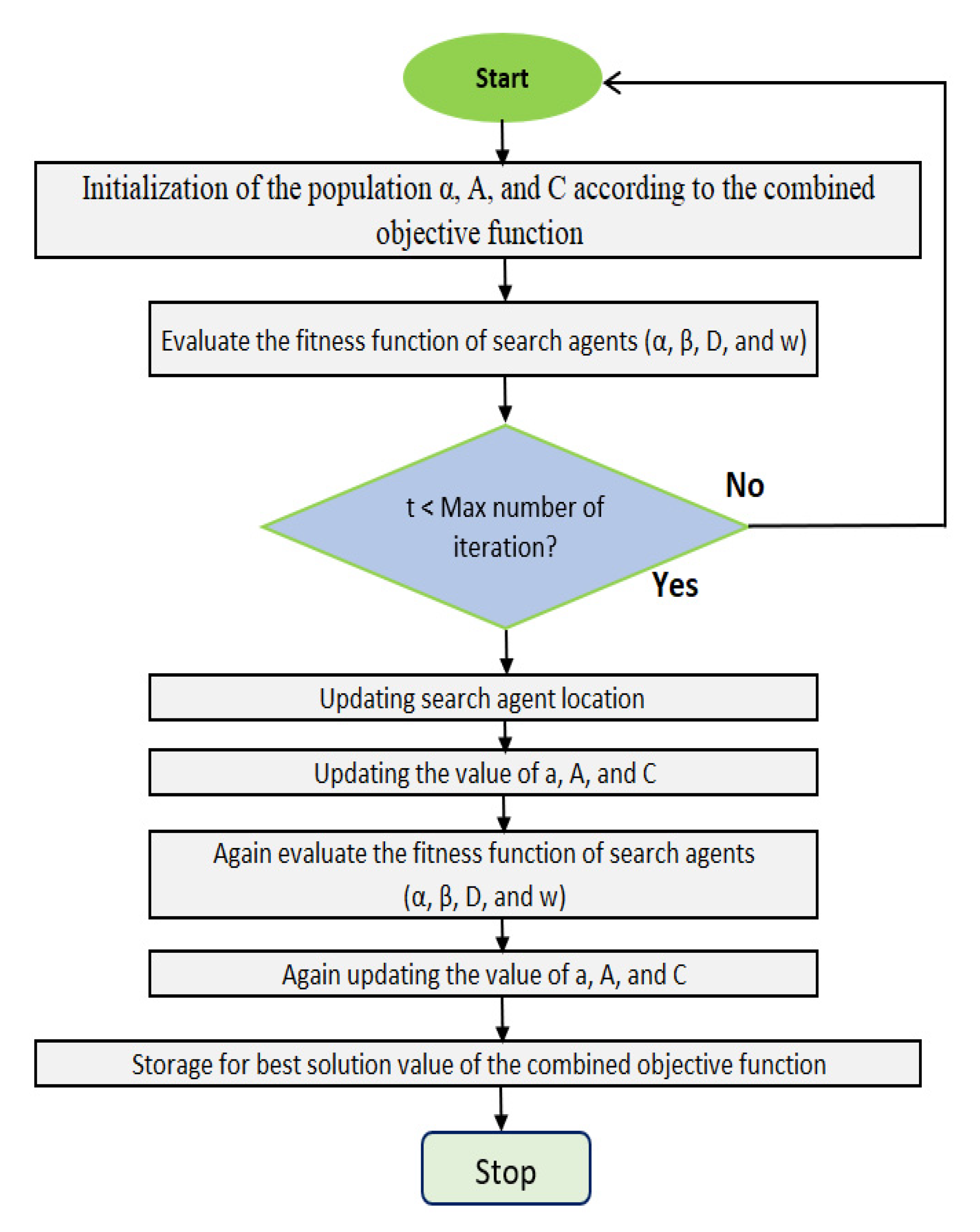
2.1.3. Grey Wolf Optimizer (GWO)

Grey wolf optimiser proposed by Mirjalili et al. (2014) depicts the interesting and systematic lifestyle of grey wolves belonging to the Canidae family. Grey wolves lie at the top of the food chain living in a pack of 5 to 12 with a social hierarchy naming alpha (α-leaders), beta (β-advisors of alpha and commands δ and ω), gamma (δ-commands ω), and omega (ω-follow every other wolf’s command). During hunting, α, β, and δ work as guides and ω follow them. During encircling of prey for hunting, it is as described by Al-Tashi et al. [56]

$$\overrightarrow{X} \left(t+1\right)=\overrightarrow{X_p}\left(t\right)+\overrightarrow{A}·\overrightarrow{D}$$

(11)

$$\overrightarrow{D}=\left|\overrightarrow{C}\cdot \overrightarrow{X_p}\left(t\right)- \overline{X} \left(t\right)\right|$$

(12)

where $t$ indicates the current iteration, $\overrightarrow{A}$ and $\overrightarrow{C}$ are coefficient vectors, $\overrightarrow{X_{\mathrm{p}}}$ is the prey’s positions vector, $X$ is the position of the wolves in d dimensional space, as d is the variable number. $\overrightarrow{A}$and $\overrightarrow{C}$ can be calculated as the following:

$$\overrightarrow{A}=2\overrightarrow{a}·\overrightarrow{{\mathrm{r}}_1}-\overrightarrow{a}$$

(13)

$$\overrightarrow{C }=2·\overrightarrow{{\mathrm{r}}_2}$$

(14)

where $\overrightarrow{{\mathrm{r}}_1}$and $\overrightarrow{{\mathrm{r}}_2}$are vectors randomly in [0, 1] and $\overrightarrow{a}$ is a set vector that linearly decreases from 2 to 0 over iterations. In the hunting process, α, β, and δ command and ω follow them modifying their positions as required by the pack until a suitable position or, in this case, a solution is achieved. The position selection can be calculated as

$$\overrightarrow{X} \left(t+1\right)=\frac{\overrightarrow{{\mathrm{x}}_1+{\mathrm{x}}_2+{\mathrm{x}}_3}}{3}$$

(15)

where ${\mathrm{x}}_1,{ \mathrm{x}}_{2,}{ \mathrm{and} \mathrm{x}}_3$ can be defined as:

$$\overrightarrow{{\mathrm{x}}_1}=\overrightarrow{X_{\alpha }}-A_1·(\overrightarrow{D_{\alpha })}$$

(16)

$$\overrightarrow{{\mathrm{x}}_2}=\overrightarrow{X_{\mathsf{\beta }}}-A_2·(\overrightarrow{D_{\mathsf{\beta }})}$$

(17)

$$\overrightarrow{{\mathrm{x}}_3}=\overrightarrow{X_{\mathsf{\delta }}}-A_3·(\overrightarrow{D_{\mathsf{\delta }})}$$

(18)

where ${\mathrm{x}}_1,{\mathrm{x}}_2,$ and ${\mathrm{x}}_3$ are the best solutions at iteration $t$, $A_1, A_{2,} \mathrm{and} A_3$ can be calculated using Equation (13) and $\overrightarrow{D_{\alpha }}, \overrightarrow{D_{\beta }}$and $\overrightarrow{D_{\delta }}$ calculated from Equation (19) and $\overrightarrow{C_1}, \overrightarrow{C_2}$and $\overrightarrow{C_3}$ from Equation (14)

$$\begin{array}{c}\overrightarrow{D_{\alpha }}=\left|\overrightarrow{C_1}\cdot {\overrightarrow{X}}_{\alpha }-\overrightarrow{X}\right|\\ \overrightarrow{D_{\beta }}=\left|\overrightarrow{C_2}\cdot {\overrightarrow{X}}_{\beta }-\overrightarrow{X}\right|\\ \overrightarrow{D_{\delta }}=\left|\overrightarrow{C_3}\cdot {\overrightarrow{X}}_{\delta }-\overrightarrow{X}\right|\end{array}$$

(19)

In the main paper, to tune exploration and exploitation $\overrightarrow{a}$ vector is suggested to decrease for each dimension linearly proportional to the number of iterations from 2 to 0. The equation is as follows, and ter is the optimisation total iterations number:

$$\overrightarrow{a}=2-t·\frac{2}{{\mathit{max}}_t\mathit{ter}}$$

(20)

Figure 1 illustrates the flowchart of the grey wolf optimisation algorithm. The figure shows that only one wolf can conduct a mating action in a wolf pack. It is not required for the alpha (α) wolf to be the strongest wolf in the pack, but the wolf must have the finest management skills. The beta (β) wolf possesses the group’s second-best command. The wolf supports each other and serve as a liaison with all other wolves in the pack. The second is the delta (Δ) and omega (ω) wolves, respectively, maintaining the group’s diminishing authority level. The wolf is the group’s lowest level of the hierarchy, and it obeys the orders and instructions of a wolf. The GWO method uses four sorts of grey wolves for the simulation, representing the four fitness functions.

2.1.4. Particle Swarm Optimiser (PSO)

The particle swarm optimiser algorithm is a population-based stochastic optimisation inspired by social and psychological considerations [57]. The PSO relates to swarm intelligence principles, which imitate the social behaviour of flocking birds or schooling fish. The algorithm has gained popularity due to its several favourable properties, including its basic structure, resilient mobility, and ease of implementation [58,59], which enable the training of various intelligent models. Each particle is considered a plausible solution in the search space of an optimisation problem. The control parameters determine the convergence of particle trajectories, keeping track of each particle’s unique best fitness value, locating the global best particle, and updating each particle’s location and velocity. If convergence is not achieved, the iterative process is repeated until either the optimisation problem converges to an optimal solution, or the maximum number of iterations is reached. The number of particles is 10, with a maximum number of iterations of 150. The maximum and minimum bond inertia weights were 0.9 and 0.4, respectively.

2.1.5. Atom Search Optimiser (ASO)

Zhao et al. [60] introduced Atom Search Optimisation (ASO) as a new metaheuristic algorithm in 2019. The ASO simulates the fundamental concepts of molecular dynamics and atom movement principles, such as potential function characteristics, contact force, and geometric constraint force. In ASO, each atom keeps track of two vectors: position and velocity. When it comes to binary optimisation, the atoms only have to deal with two numbers (“1” or “0”). As a result, a means to leverage the atom’s velocity to alter the position from “0” to “1” or vice versa should be discovered. Previous research has shown that the transfer function helps convert a continuous optimisation algorithm to a binary one [61]. During the initial iterations of ASO, each atom interacts with others via attraction or repulsion. Repulsion can help avoid over-concentration of atoms and premature algorithm convergence, improving exploration capability across the search space. As iterations progress, the repulsion becomes weaker, and the attraction becomes more robust, indicating that exploration diminishes, and exploitation grows. Finally, each atom interacts with other atoms by attraction, ensuring that the algorithm has a lot of power to use.

2.1.6. Ant Colony Optimiser (ASO)

Dorigo and Caro [62] proposed Ant Colony Optimization (ACO), which is technically motivated by the behaviours of ant colonies. We used an ACO algorithm to identify features as a comparing approach in this work. According to the ACO algorithm’s theory, when ants discover a sign of food, they leave a fragrant chemical known as a pheromone to mark the trail [63]. When an ant seeks food, it follows the pheromone trail. Additionally, this ant deposits pheromones along the path, allowing other ants to follow suit. When an ant must choose between two roads, it chooses the one with a high pheromone level, indicating that more ants have travelled the path. It is a question of convenience for the ants; shorter trails become more fragrant than longer paths. If an ant does not follow a trail, the pheromone degrades over time. As a result, the intensity of the pheromone is diminished [64], and over time, all ants will take the shorter route to food. Finally, “pheromone evaporation” and “probabilistic path selection” supply information to ants for them to identify the shortest food path. The notions enable elasticity in the solution of optimisation problems. In a nutshell, an ant can use the information contained in the bodies of other ants to select a more practical choice.

2.1.7. Comparing Predictive Models

Three machine learning models were also included in determining a viable approach to machine learning and a feature selection approach. Multiple Linear Regression (MLR) seeks to model the relationship between two or more explanatory variables and a target variable. It aids in determining the extent to which variables vary [65]. Support Vector Regression (SVR) is a machine learning kernel approach is used for various tasks, including forecasting time series. SVRs that employ kernels can also learn the training data’s non-linear trend. Three SVR models are available, each with a unique kernel (RBF, poly, and linear) [66]. Additionally, the SVR model has been used in a variety of research applications, including precipitation [67], solar radiation [68], wind energy [69], flood forecasting [68,70], evaporation [71], and crop yield [72,73] prediction.

Breiman [74] developed the random forest (RF) model, and it contains regression and classification methods. The RF model assembles tree predictors linked to distinct values of randomly sampled random vectors. The model creates decor-related decision trees during the training phase, and the overall model output is derived by averaging the output values of all the individual trees [75]. The bootstrap resampling process generates a new set of training data from the initial training sample set N, and then K decision trees are used to construct bootstrap-set random forests. The complete specifications for the RF model may be found here [45]. RF is a collection (ensemble) of fundamental tree predictors. Each tree can generate a response given a set of predictor values [75]. The random forest method has been successfully implemented in predicting different crop yields worldwide [75,76].

3. Study Area and Data

3.1. Study Area and Wheat Yield Data

This study focused on a wheat yield prediction problem in South Australia, the fourth largest state in southern central Australia. Australia has a Mediterranean climate with an abundance of rain suitable for rainfed agriculture and crops like wheat. Wheat is the largest broadacre winter crop typically sown from May to June and harvested by November and December [26,77]. In the 2019–2020 financial year, 14 million tonnes of wheat were harvested in Australia, 18% less than the previous year, and 2.689 million tonnes of wheat were produced in South Australia (SA) [78]. Several climatic conditions, such as rainfall, soil moisture, temperature, solar radiation, humidity, etc., determine wheat production and are essential inputs to empirical and process-based models [26]. Delayed harvest due to a series of heavy rainfall in November and flooding in some regions is likely to cause a fall in wheat production in 2021–2022, which leads to poor grain quality [79]. Wang et al. [80] showed that climate variability could impact wheat production by 31% to 47%.

For this study, the average yearly wheat yield data for South Australia (SA) from 1990 to 2020 was downloaded from the Australian Bureau of Agricultural and Resource Economics and Sciences (ABARES) (http://apps.agriculture.gov.au/agsurf/, 29 December 2021). The dataset was acquired through farm surveys where the farm population ranged from 1967 to 9018 farms, and the sample was between 73 and 206 farms. The farm population was stratified based on operation size using the estimated value of the agricultural operation. The size of each stratum was decided using the Dalenius–Hodges method, while the sample was assigned to each stratum using a mixture of the Neyman allocation [81]. This dataset has been a prime source of information on the current and historical economic performance of Australian farm business units and has been used to undertake research and analysis on a range of industry issues and government policy areas.

It is worth to mention that South Australia’s cropping zones are of three types, namely pastoral (411: SA North Pastoral), wheat-sheep (421: SA Eyre Peninsula; 422: SA Murray Lands and the Yorke Peninsula), and high rainfall (431: SA South East) zone [82]. Except for the Murray lands, where rainfall was generally average, most farming districts in South Australia experienced below-average rainfall in September. Most crops’ yield potential was increased by adequate rainfall and mild temperatures in October, especially those sown later. However, the recovery in growth conditions in October came too late for crops in the upper regions of the Eyre Peninsula and the Yorke Peninsula, which had been harmed by dry conditions in early spring [79].

3.2. Predictor Variables

The monitoring of crop conditions using remote sensing is being used extensively to assess crop conditions, soil moisture, and the probability of natural disasters such as pest infestation, drought, and precipitation [83]. Ahmed et al. [55,63,84] has discussed the importance of satellite-based remote sensing to forecasting and constant monitoring of soil moisture and its importance in agriculture and human activities. Several other studies have also projected the correlation between weather conditions and remote sensing information to address the situation [26,85]. This study collected satellite data from NASA’s GES-DISC Interactive Online Visualization and Analysis Infrastructure (GIOVANNI) repository from 1991 to 2020. Specifically, the study used Modern-Era Retrospective Analysis for Research and Applications, Version 2 (MERRA-2), whose data set spans 1980 to the present.

Along with the improvements to meteorological assimilation, MERRA-2 makes significant progress towards the Earth System. MERRA-2 is the first long-term global reanalysis that incorporates space-based aerosol observations and their interactions with other physical processes in the climate system. The MERRA-2 model has a native spatial resolution of 0.5 lat × 0.625 long and four temporal resolutions: daily, hourly, 3-hourly, and monthly. The study used 32 monthly hydro-climatic variables converted to the yearly data to be correlated with wheat yield, as tabulated in

Table 1. A description of the 32 predictors from the MERRA-2 satellite system used to design the hybrid GWO-CEEMDAN-KRR model for wheat yield prediction (tonnes) in South Australia. The feature selections were undertaken using GWO, ACO, PSO, and ASO, and a √ shows the selected feature, whereas a × shows the rejected feature.

Information of Satellite Derived Variables			Results of Feature Selection
Notation	Description	Units	GWO	ACO	ASO	PSO
Q	Specific humidity @1000 hPa	kg/kg	×	√	√	√
TA	Air temperature monthly @1000 hPa	K	√	√	√	×
Q10	10-m specific humidity	kg/kg	×	√	√	√
TO3	Total column ozone	Dobsons	√	×	×	√
T2X	2-m air temperature-daily max	K	√	×	√	√
T2A	2-m air temperature-daily mean	K	√	√	√	√
T2M	2-m air temperature-daily min	K	√	×	√	√
LE	Total latent energy flux	W/m−2	×	×	×	×
PR	Total precipitation	Kg/m2	×	√	√	×
TA	Surface air temperature monthly	K	×	√	×	√
GRN	Greenness fraction	-	√	×	√	×
SW	Surface soil wetness	-	×	√	×	√
LAI	Leaf area index	-	√	×	×	√
ALB	Surface albedo	-	√	×	×	√
CL	Total cloud area fraction	-	√	×	√	×
SSF	Surface incoming shortwave flux	W/m−2	×	×	×	×
Q250	Specific humidity at 250 hPa	kg/kg	√	×	√	×
Q500	Specific humidity at 500 hPa	kg/kg	×	×	√	√
Q850	Specific humidity at 850 hPa	kg/kg	×	√	√	√
Q10	10-m specific humidity	kg/kg	×	×	√	√
Q2	2-m specific humidity	kg/kg	√	×	√	×
SLP	Sea level pressure	hPa	√	√	√	×
T10	Temperature at 10 m above surface	K	×	×	√	×
T2	2-m air temperature	K	×	√	√	√
TS	Surface skin temperature	K	√	√	×	×
U10	10-m eastward wind	m/s	×	√	√	×
U2	2-m eastward wind	m/s	√	×	√	×
U50	Eastward wind at 50-m	m/s	√	×	√	√
V10	10-m northward wind	m/s	√	√	√	√
V2	2-m northward wind	m/s	√	√	√	√
V50	Northward wind at 50-m	m/s	√	√	√	×
A	Area	Ha	×	×	√	×
Total Number of Selected Features			18	15	24	17

. The predictor variables were extracted as area-averaged of the time series data, as the target data (i.e., wheat yield) was provided for the whole of South Australia. Figure 1 depicts the atmospheric domain of South Australia between 127.44°E, 38.79°S, and 141.77°E, 23.76°S to extract the area-averaged wheat yield data. Satellite data collection has significant advantages overground stations regarding costs and coverage range. Local factors significantly impact ground stations and do not typically have a logical distribution system [86]. On the other hand, satellite remote sensing is not impacted by local conditions and captures data with a uniform cell size throughout the world. Interestingly, satellite data tracks crop growth conditions and gradually captures the variability in yield as the growing season progresses, and their contribution to yield prediction peaks during the growing season’s peak [26,87].

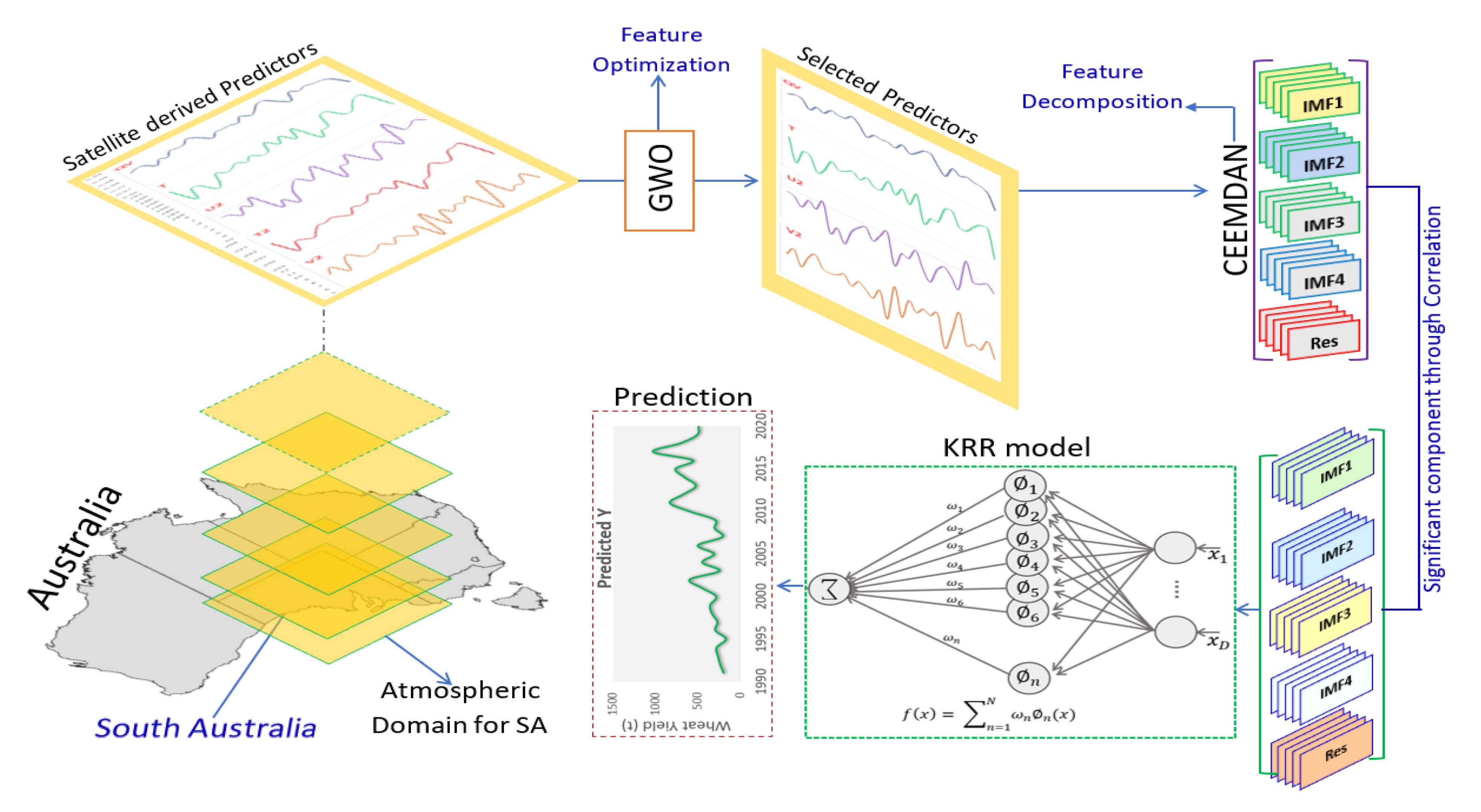
3.3. Development of GWO-CEEMDAN-KRR Model

The proposed GWO-CEEMDAN-KRR model was developed on a personal computer (PC) equipped with an Intel i7 processor running at 3.6 GHz and 16 GB of RAM. A publicly available machine learning library, scikit-learn [88,89] using Python, was employed to execute the KRR model for the proposed framework. An implementation of the feature optimisation (i.e., GWO, ACO, ASO, and PSO) has been developed using MATLAB R2020b. The CEEMDAN method is executed with the programming language software R. To visualise further the anticipated wheat yield, tools such as matplotlib [90] and seaborn [91] are used, in addition to standalone methods. The following steps were carried out to develop the proposed GWO-CEEMDAN-KRR model.

Step 1: The 31 predictor variables obtained from the MERRA-2 satellite model were combined to screen the best-correlated input predictors using grey wolf optimisation (GWO) techniques. The use of GWO resulted in the best-selected predictors being used for feature decomposition. The optimal values of four selected feature selection algorithms are tabulated in

Table 2. The optimal parameter for the optimization algorithms such as grey wolf optimization (GWO), ant colony optimization (ACO), atom search optimization (ASO), and particle swarm optimization (PSO).

Characteristics	Optimal Value
Grey Wolf Optimization (GWO)
Number of wolves	10
Maximum number of iterates	100
Curve	Convergence
Ant Colony Optimization (ACO)
Number of ants	10
Maximum number of iterations	100
Coefficient control tau	1
Coefficient control eta	2
Initial tau	1
Initial beta	1
Pheromone	0.2
Coefficient	0.5
Atom Search Optimization (ASO)
Number of particles	10
Maximum number of iterations	100
Depth weight	50
Multiplier weight	0.2
Particle Swarm Optimization (PSO)
Number of particles	10
Maximum number of iterations	150
Cognitive factor	2
Social factor	2
Maximum velocity	6
Maximum bound on inertia weight	0.9
Minimum bound on inertia weight	0.4

. For the GWO, the optimal number of wolves is fixed at 10 with 100 iterations. Similarly, ACO, PSO, and ASO algorithms provide essential information on selecting significant predictor variables.

Table 1 shows the optimal set of satellite-derived features selected by GWO, ACO, ASO, and PSO methods.

Table 1 demonstrates that the GWO optimised diversified hydro-climatological variables for the predictive model.

Table 2 provides the optimum parameters of the GWO, ACO, ASO, and PSO algorithms.

Step 2: In this step, each of the GWO optimised predictor variables was resolved into 4-IMFs (i.e., IMF1, IMF2, IMF3, and IMF4) and 1-residual (RES) using the CEEMDAN method (18 × 5 = 90 IMFs in total). Gaussian Noise realisations (N = 500) and the provided amplitude in terms of added white noise (=0.2). The implementation of the CEEMDAN process is in Figure 1. The decomposed component was then correlated with the variable (i.e., wheat yield) by Pearson’s correlation, and the most highly correlated components were chosen as the target components for the KRR model.

Step 3: The selected predictor IMFs are normalised to minimise the overinfluence of one input to another. Using the following equation, all variable features were normalised to ensure that they received proportional attention in network training [0, 1] [26,27,28].

$${\delta }_{norm}=\frac{\delta -{\delta }_{min}}{{\delta }_{max}-{\delta }_{min}}$$

(21)

In Equation (21), $\delta$ is the respective variable, ${\delta }_{min}$ is the minimum variable, ${\delta }_{max}$ is the maximum, and ${\delta }_{norm}$ is the normalised variable. After normalising the variables, the datasets are partitioned into training (1991–2010), validation (2011–2016), and testing (2017–2020) subsets. The data partitioning is done by the trial-and-error method.

Figure 2 shows the methodological steps of the proposed GWO-CEEMDAN-KRR model.

Step 4: To predict the wheat yield of South Australia, this study developed the KRR model to use the predictors’ data in step 3. GridSearchCV was used to create an optimal architecture of the KRR model (regularisation strength = 1.5; gamma parameter = None, with a degree of the polynomial kernel = 3 and kernel = rbf). The performance of the proposed model was compared to that of standalone machine learning models.

3.4. Predictive Model Evaluation

The robustness of the proposed machine learning model (i.e., GWO-CEEMDAN-KRR) and the benchmark model is assessed using numerous performance metrics, e.g., Pearson’s Correlation Coefficient (r), root mean square error (RMSE), and normalised root means square error (RMSE). Due to geographic differences between the study stations, we also employ the relative error-based metrics: i.e., relative MAE (denoted as RMAE), to compare geographically and climatologically diverse wheat yield sites. The accuracy of any predictive model is evaluated by comparing its predicted test values to the actual test results. The relative index of agreement (d_rel) can be a more sophisticated and compelling measure form than the RMSE when the error distribution in the tested data is Gaussian [92]. A sensitivity analysis was undertaken to evaluate the contributing response to the anticipated Y of the provided set of predictor variables to verify the prediction models created in our study. The goal was to see which predictor variables contributed the most to modelling the monthly evaporative loss value. Following previous research [93,94,95], we calculated the sensitivity % of the output (E) to each predictor (x) variable as follows:

$$Z_{\mathrm{i}}=f_{max}\left({\mathrm{x}}_{\mathrm{i}}\right)-f_{mi\mathrm{n}}\left({\mathrm{x}}_{\mathrm{i}}\right)$$

(22)

$$S_{\mathrm{i}}=\frac{Z_{\mathrm{i}}}{{{\displaystyle \sum }}_{\mathrm{i}=1}^{\mathrm{n}}{Z}_{\mathrm{j}}}\times 100$$

(23)

where f_max(x_i) and f_max(x_i) are, respectively, the maximum and the minimum predicted Y over the ith domain, where other variables are equal to their mean values. Z_j is the predicted value

4. Results

In this study, a hybrid KRR predictive model denoted as GWO-CEEMDAN-KRR is developed and evaluated for its capability to predict wheat yield (Y) in South Australia. The performance accuracy of wheat yield prediction is evaluated in comparison with several comparing models (i.e., CEEMDAN-MLR, CEEMDAN-RF, and CEEMDAN-SVR) and standalone methods (e.g., KRR, RF, MLR, and SVR) with all models employing four competitive feature optimisation algorithms (i.e., GWO, ACO, ASO, and PSO). The outcomes of the newly designed hybrid KRR predictive models were evaluated using statistical score metrics in conjunction with the diagnostic plots of both the observed and the predicted Y for the testing datasets.

Comparing the observed and predicted Y test data, we note that the newly developed CEEMDAN-KRR model can generate the highest value of R (showing a good degree of agreement between observed and predicted Y) while also generating the lowest values of NRMSE using the grey wolf optimisation method, according to the findings in

Table 3. Evaluation of the hybrid CEEMDAN-KRR vs. the benchmark (i.e., CEEMDAN-MLR, CEEMDAN-RF, CEEMDAN-SVR) models and their respective standalone counterpart (i.e., KRR, MLR, RF, and SVR) models. The r and normalized root mean square error (NRMSE) is computed between predicted and observed Wheat Yield (Y, tonnes) South Australia.

Predictive Model	R	NRMSE
GWO–Objective Feature Selection Method
CEEMDAN-KRR	0.998	0.437
CEEMDAN-MLR	0.896	1.144
CEEMDAN-RF	0.751	0.589
CEEMDAN-SVR	0.840	0.614
ACO–benchmark method
CEEMDAN-KRR	0.990	0.452
CEEMDAN-MLR	0.860	1.122
CEEMDAN-RF	0.847	0.531
CEEMDAN-SVR	0.681	0.743
ASO–benchmark method
CEEMDAN-KRR	0.974	0.738
CEEMDAN-MLR	0.866	0.659
CEEMDAN-RF	0.768	0.601
CEEMDAN-SVR	0.849	0.523
PSO–benchmark method
CEEMDAN-KRR	0.980	0.475
CEEMDAN-MLR	0.973	0.655
CEEMDAN-RF	0.784	0.689
CEEMDAN-SVR	0.929	0.525
Standalone
KRR	0.738	0.761
MLR	0.963	2.992
RF	0.882	0.653
SVR	0.758	0.710

. The GWO-CEEMDAN-KRR model with GWO produced R ≈ 0.998, NRMSE ≈ 0.437 %, followed by ACO-CEEMDAN-KRR (R ≈ 0.990 and NRMSE ≈ 0.452%), PSO- CEEMDAN-KRR (R ≈ 0.980 and NRMSE ≈ 0.477%) model that also produced substantially good, yet a lower performance relative to the GWO-CEEMDAN-KRR model. We discovered that an MLR model could produce better performance with a high R-value (0.963) in the standalone model. However, this model still underperforms the objective GWO-CEEMDAN-KRR model. Therefore, we note that the proposed CEEMDAN-KRR model using the grey wolf optimisation feature selection with an appropriate feature decomposition using the CEEMDAN) method provided the most satisfactory performance. Regarding the benchmark models’ poor performance (as shown in Table 3), the newly proposed hybrid KRR (i.e., GWO-CEEMDAN-KRR) predictive model has proven to be a superior tool for predicting the wheat yield in South Australia using a carefully selected set of satellite-based predictor variables.

The predictive performance of the proposed hybrid GWO-CEEMDAN-KRR model is further evaluated by examining the relative error values (i.e., RMAE) and coefficient of determination (R²) between the observed and predicted wheat yield in the testing phase as shown in Figure 3. According to Figure 3, the newly developed CEEMDAN-KRR model, with GWO algorithm, has the lowest percentage of RMAE (≈32%) and the highest R² value (≈0.997), which is an impressive result compared with the same model with other optimisation techniques. We also noted that the GWO method could produce the best performance when integrated with the KRR-based predictive model compared with the different feature selection techniques.

Interestingly, the KRR model performs best when the predictor variables are decomposed with the CEEMDAN method using all optimisation techniques. Our results range between 32% and 36% regarding the RMAE value. The improvement in the prediction performance is more evident after applying the feature decomposition (i.e., CEEMDAN) and the feature optimisation (i.e., GWO) techniques. By these results, the hybrid CEEMDAN-KRR model seems to outperform the comparison benchmark models and the standalone machine learning models, demonstrating superior performance.

It is worth noting that this study has employed two distinct algorithms (one for feature selection, namely the GWO, and the other for decomposition of selected features, namely the CEEMDAN) to improve the overall performance of the hybrid KRR-based predictive model. As a result, in Figure 4, we illustrate the effects of incrementally applying the CEEMDAN and different optimisation methods such as GWO, ACO, ASO, and PSO as the data pre-processing and the feature selection methods on the percentage change in error (i.e., RMAE) and percentage change in Willmott’s Index (i.e., d_rel) from their respective standalone models. The RMAE (%) values of the CEEMDAN-KRR model, which incorporates a GWO method for satellite predictor variable feature selection, appear to decrease by ≈20%. For drel, this is a 35% increment from the standalone KRR model. Moreover, for the case of the ACO feature selection method, the change of RMAE and d_rel is 16 and 34%, for ASO, this change is 18 and 31%, and for PSO, the change is 10 and 30%, accordingly relative to the standalone KRR model. The other models, such as the SVR, RF, and MLR, showed a minimum improvement in utilising the four optimisation techniques and the CEEMDAN data decomposition technique. This indicates that incorporating the CEEMDAN and the GWO methods can improve the model’s predictive capability in simulating the wheat yield tested data values. This is notable by these values outperforming the indices generated for the comparison model by a significant margin. Therefore, this exemplifies that the proposed hybrid predictive model is more accurate than competing methods used to predict wheat yield.

To demonstrate a superior performance of the proposed GWO-CEEMDAN-KRR and its standalone counterpart models, we have also examined the prompting percentage of the correlation coefficient (ΔR), RMAE (ΔRMAE), and NRMSE (ΔNRMSE) for wheat yield prediction, as illustrated in Figure 5. Note that the promoting percentage, presented as the incremental performance (Δ) of the objective model over the competing approaches, aims to evaluate the difference in the R, RMAE, and NRMSE of the GWO-CEEMDAN-KRR against the other models. In general, the metrics ΔR, ΔRMAE, and ΔNRMSE are used to demonstrate a performance edge of the preferred (i.e., GWO-CEEMDAN-KRR) model over the comparative counterparts. Figure 5 shows the results as for the case of ΔR, the improvement is found to be ≈1% to 25%; for the case of ΔRMAE, the improvement is ≈2 to 60%. Likewise, improving prediction performance in terms of ΔNRMSE also demonstrates significant improvements. This demonstrates that our proposed model (i.e., GWO-CEEMDAN-KRR) was the most responsive in the prediction process.

The discrepancy ratio (Dr) is used to further investigate the proposed model’s robustness. In general, the discrepancy ratio (Dr) measures whether a model overestimates or underestimates a simulated wheat yield value. The Dr value that begins with a “one” indicates that an exact prediction can be made for a specific observation. According to Figure 6, the GWO-CEEMDAN-KRR model shows that the distribution of Dr is within a ±30% band error for observation of the testing phase. As determined by the discrepancy ratio, hybrid machine learning approaches were the most accurate predictive models compared to other models on the same basis. As shown in Figure 7, a scatter plot is used to perform an additional evaluation of the hybrid predictive model (i.e., CEEMDAN-KRR) where the GWO algorithm and the previous evaluation. The scatter plot is plotted with the goodness-of-fit between the predicted and observed Y, and a least-square fitting line to represent the relationship between the two variables. The suggested model outperforms the standalone model with an R² value significantly higher than the baseline model.

Concerning the proposed model with GWO algorithm, it performed significantly better than the other feature optimisation algorithms (i.e., ACO, ASO, and PSO), registering magnitudes that were the closest to unity (m|R² 0.997|0.167), followed by the CEEMDAN-KRR model with ACO (0.980|0.157). For the case of standalone KRR, the unity has far deviated from the proposed model’s exhibits statistically significant performance with the proposed model. Therefore, the learning hybrid CEEMDAN-KRR model with the GWO algorithm is exceptionally well suited for predicting wheat yield for South Australia.

The performance of Wheat prediction using GWO-CEEMDAN-KRR that is shown in Figure 8a (ECDF) examines the plots of various prediction skills using an empirical cumulative distribution function (ECDF). Comparing the performance of the proposed hybrid KRR model to the benchmark models, the generated error ranged from 50 to 300 within the 95 per cent percentile, demonstrating that the CEEMDAN-KRR model with the GWO model was the most accurate and responsive wheat yield prediction model. A Taylor diagram provides a more specific and conclusive argument about how strongly the predicted and observed Y are correlated than a simple correlation coefficient. As illustrated in Figure 8b, the output of the GWO-CEEMDAN-KRR model is significantly closer to the observation than the output of other comparing models, as indicated by the Taylor diagram. The GWO outperformed other models’ optimised CEEMDAN-KRR model to achieve the observed values’ closest match; however, the proposed model outperformed against other counterpart models. The study site had a higher R-value than the observed Y for the proposed CEEMDAN-KRR model, further supporting the findings of improved performance by this model, which was previously reported.

In addition to understanding the contribution of the input variables to the yield prediction, a sensitivity analysis of individual variables was performed. Figure 9 shows the results of sensitivity analysis for the proposed GWO-CEEMDAN-KRR model. It can be observed that almost all the parameters selected by GWO were significant, ranging from 20% to 33%. Specifically, the leaf area index (LAI) had the highest sensitivity, which is endorsed by other researchers [96,97]. However, inputs like V50, V10, V2, T2A, TS, and Q2 show a similar sensitivity percentage, ranging from 28% to 31%. The high sensitivity of the northward wind values is substantial, which is needed to be explored in further study. Moreover, surface albedo and other meteorological variables were also found to be significant in predicting wheat yield in South Australia.

5. Discussion

The useful information derived from space combined with advanced machine algorithms enabled the development of more accurate near-real-time forecasts for different crops at different scales [98,99]. The findings from this study clearly showed that spatial information derived from MERRA-2 combined with the hybrid CEEMDAN-KRR model could provide an accurate forecast tool for wheat yield in Australia. The high accuracy of the proposed model has been proven through the reported model performance using different evaluation criteria and benchmark models. In this study, the CEEMDAN-KRR model with GWO generated R (0.998), and NRMSE (0.437%) outperformed other hybrid and standalone models. Furthermore, the integration of the GWO technique has indicated the most important predictors among 32 variables for wheat yield forecast. While the present study contributes to the current research avenue, several limitations, challenges, and suggestions for further research are discussed.

This study used the space-based MERRA-2 dataset to exploit many variables related to atmospheric, weather, and canopy conditions. However, this dataset’s coarse resolution (0.5° × 0.625°) might affect the forecast accuracy of wheat yield. The predictor variables obtained as area-averaged of the time series data for the whole of South Australia’s atmospheric domain would minimise the effect. Moreover, integrating vegetation indices (VIs), land surface temperature (LTS), and weather variables acquired from higher spatial resolution satellite data is highly recommended to overcome this issue. Multi-temporal VIs such as Normalized Difference Vegetation Index (NDVI) and Enhanced Vegetation Index (EVI) derived from MODIS (250 m), Landsat (30 m), and Sentinel (10 m) data have been successfully explored in predicting crop yield [100,101]. Furthermore, the composited products (e.g., from MODIS) on a near real-time basis of 8 days, 16 days, and months can overcome the cloud cover problem and, thus, improve the model performance. In addition, gridded precipitation retrieved from the Climate Hazards Group Infrared Precipitation with Stations (CHIRPS) dataset (~5.5 km) can provide helpful information to develop crop yield forecast models [102].

One of the main challenges of using satellite-based data to predict crop yield at a regional level is the lack of cropland cover masks. Zhang et al. [103] reported a consistent improvement in yield prediction using crop-specific masks at all regions and scales. In contrast, Shao et al. [104] claimed that using available cropland masks (e.g., summer crop or cultivated crops) generated similar results to using an annual corn-specific mask. It is also worth noting that the MERRA-2 dataset used in this study was extracted in the atmospheric domain of South Australia between 127.44°E, 38.79°S and 141.77°E, 23.76°S to extract the area-averaged wheat yield data, which potentially affects the forecast results. Therefore, it is interesting to explore whether the wheat crop’s growing boundary could enhance the forecast accuracy.

Another factor that may affect the model performance is the algorithms used for modelling relationships between crop yield and predictors. Methods such as RF or SVM might not perform well with time-ordered data such as multi-temporal VIs and weather variables [102]. The authors demonstrated that the LSTM neural network model outperformed the multivariate OLS regression and random forest in soybean yield prediction. Our results also showed that the CEEMDAN-KRR model is superior to MLR, RF, and SVR-based models. In addition, deep learning methods are up-and-coming for the crop yield prediction problem [105,106]. Therefore, future research can consider using space-based datasets and deep learning approaches combined with automatic feature extraction to improve yield forecasts. This study has established an essential framework for building smart farming services. The high accuracy of crop yield prediction information in different climatic conditions using the proposed model is an essential element that helps agricultural producers and other stakeholders improve decision-making. In addition, this research helps rural areas where gauge-based observations are not always available. This is because satellite data can be used to help this research.

6. Conclusions

The prediction of wheat, subsistence, or commercial agricultural commodities using freely available satellite data and remote sensing methods can add value to new initiatives in precision agriculture. The active promotion of Agriculture 4.0, an Austrade strategy, showcases our competitive advantage in agtech and foodtech to a global audience through digital practices such as modelling crop yields through machine learning methods. This paper has developed and implemented a hybrid machine learning algorithm with an artificial intelligence methodology for wheat yield prediction in South Australia. The new approach uses a feature selection strategy and the subsequent decomposition of the selected features as an optimisation algorithm to improve the proposed Kernel Ridge Regression (KRR) and a set of competitive compression models. To train the prescribed models, we have used thirty-two predictors derived from the MERRA-2 satellite datasets to encapsulate the features to model wheat yield and quantify the relationships between satellite-derived information and ground-based wheat yield. Our novel method combined the CEEMDAN, a feature decomposition method, and the grey wolf optimisation, a feature selection method, to improve kernel ridge regression prediction accuracy. The proposed hybrid GWO-CEEMDAN-KRR model, composed of five distinct modules for optimal accuracy, was tested on area-aggregated wheat yield data in South Australia. A common problem in data-driven modelling was solved when the GWO algorithm was used in the machine learning model. It reduced the number of predictor variables to solve this problem.

According to the results of this study, the proposed hybrid CEEMDAN-KRR model demonstrated the best performance in predicting wheat yield when it was optimised by the GWO method. The high R-value of the CEEMDAN-KRR predictive model, which ranged from 0.0980 to 0.998, and the low NRMSE value, which ranged from 0.437 to 0.475, supported the different feature selection techniques of the model’s superior testing performance. More precisely, the CEEMDAN-KRR model improved with the GWO feature selection algorithm and registered the best performance. The scatterplot revealed that the merits of the CEEMDAN-KRR model with GWO are the closest to unity, supporting the applicability of the newly designed hybrid CEEMDAN-KRR model in real-time applications. Therefore, we ascertain that the proposed model can address a wide range of complex or challenging prediction tasks in agriculture and can be a helpful method for predicting other variables such as rainfall, wind speed, flood, or drought index. Global climate model (GCM) datasets could be used in the future to predict crop yields under different global warming scenarios, assess CO₂ emissions, and measure agricultural sustainability to figure out how future climate change and climate variability will affect farming.

References

1. Pathak, H.; Aggarwal, P.K.; Singh, S. Climate Change Impact, Adaptation and Mitigation in Agriculture: Methodology for Assessment and Applications; Indian Agricultural Research Institute: New Delhi, India, 2012; Volume 302. [Google Scholar]
2. Rosenberg, N.J. Adaptation of agriculture to climate change. Clim. Chang. 1992, 21, 385–405. [Google Scholar] [CrossRef]
3. Rickards, L.; Howden, S.M. Transformational adaptation: Agriculture and climate change. Crop Pasture Sci. 2012, 63, 240–250. [Google Scholar] [CrossRef]
4. Leng, G.; Hall, J.W. Predicting spatial and temporal variability in crop yields: An inter-comparison of machine learning, regression and process-based models. Environ. Res. Lett. 2020, 15, 044027. [Google Scholar] [CrossRef]
5. Iizumi, T.; Ramankutty, N. How do weather and climate influence cropping area and intensity? Glob. Food Secur. 2015, 4, 46–50. [Google Scholar] [CrossRef] [Green Version]
6. Ruane, A.C.; Major, D.C.; Winston, H.Y.; Alam, M.; Hussain, S.G.; Khan, A.S.; Hassan, A.; Al Hossain, B.M.T.; Goldberg, R.; Horton, R.M. Multi-factor impact analysis of agricultural production in Bangladesh with climate change. Glob. Environ. Chang. 2013, 23, 338–350. [Google Scholar] [CrossRef] [Green Version]
7. Challinor, A.J.; Watson, J.; Lobell, D.B.; Howden, S.; Smith, D.; Chhetri, N. A meta-analysis of crop yield under climate change and adaptation. Nat. Clim. Chang. 2014, 4, 287–291. [Google Scholar] [CrossRef]
8. Olesen, J.E.; Bindi, M. Consequences of climate change for European agricultural productivity, land use and policy. Eur. J. Agron. 2002, 16, 239–262. [Google Scholar] [CrossRef]
9. Thornton, P.K.; Jones, P.G.; Alagarswamy, G.; Andresen, J. Spatial variation of crop yield response to climate change in East Africa. Glob. Environ. Chang. 2009, 19, 54–65. [Google Scholar] [CrossRef]
10. Alexandrov, V.; Hoogenboom, G. The impact of climate variability and change on crop yield in Bulgaria. Agric. For. Meteorol. 2000, 104, 315–327. [Google Scholar] [CrossRef]
11. Romeijn, H.; Faggian, R.; Diogo, V.; Sposito, V. Evaluation of deterministic and complex analytical hierarchy process methods for agricultural land suitability analysis in a changing climate. ISPRS Int. J. Geo-Inf. 2016, 5, 99. [Google Scholar] [CrossRef] [Green Version]
12. Aschonitis, V.; Mastrocicco, M.; Colombani, N.; Salemi, E.; Kazakis, N.; Voudouris, K.; Castaldelli, G. Assessment of the intrinsic vulnerability of agricultural land to water and nitrogen losses via deterministic approach and regression analysis. Water Air Soil Pollut. 2012, 223, 1605–1614. [Google Scholar] [CrossRef]
13. Meenken, E.; Wheeler, D.; Brown, H.; Teixeira, E.; Espig, M.; Bryant, J.; Triggs, C. Framework for uncertainty evaluation and estimation in deterministic agricultural models. Nutr. Manag. Farmed Landsc. Occas. Rep. 2020, 33, 1–11. [Google Scholar]
14. Kingsley, J.; Afu, S.M.; Isong, I.A.; Chapman, P.A.; Kebonye, N.M.; Ayito, E.O. Estimation of soil organic carbon distribution by geostatistical and deterministic interpolation methods: A case study of the southeastern soils of nigeria. Environ. Eng. Manag. J. EEMJ 2021, 20, 1077–1085. [Google Scholar] [CrossRef]
15. Holman, I.; Tascone, D.; Hess, T. A comparison of stochastic and deterministic downscaling methods for modelling potential groundwater recharge under climate change in East Anglia, UK: Implications for groundwater resource management. Hydrogeol. J. 2009, 17, 1629–1641. [Google Scholar] [CrossRef]
16. Sharma, E.; Deo, R.C.; Prasad, R.; Parisi, A.V. A hybrid air quality early-warning framework: An hourly forecasting model with online sequential extreme learning machines and empirical mode decomposition algorithms. Sci. Total Environ. 2020, 709, 135934. [Google Scholar] [CrossRef]
17. Sharma, E.; Deo, R.C.; Prasad, R.; Parisi, A.V.; Raj, N. Deep Air Quality Forecasts: Suspended Particulate Matter Modeling With Convolutional Neural and Long Short-Term Memory Networks. IEEE Access 2020, 8, 209503–209516. [Google Scholar] [CrossRef]
18. Kouadio, L.; Deo, R.C.; Byrareddy, V.; Adamowski, J.F.; Mushtaq, S.; Nguyen, V.P. Artificial intelligence approach for the prediction of Robusta coffee yield using soil fertility properties. Comput. Electron. Agric. 2018, 155, 324–338. [Google Scholar] [CrossRef]
19. Ren, J.; Chen, Z.; Zhou, Q.; Tang, H. Regional yield estimation for winter wheat with MODIS-NDVI data in Shandong, China. Int. J. Appl. Earth Obs. Geoinf. 2008, 10, 403–413. [Google Scholar] [CrossRef]
20. Franch, B.; Vermote, E.; Becker-Reshef, I.; Claverie, M.; Huang, J.; Zhang, J.; Justice, C.; Sobrino, J.A. Improving the timeliness of winter wheat production forecast in the United States of America, Ukraine and China using MODIS data and NCAR Growing Degree Day information. Remote Sens. Environ. 2015, 161, 131–148. [Google Scholar] [CrossRef]
21. Han, J.; Zhang, Z.; Cao, J.; Luo, Y.; Zhang, L.; Li, Z.; Zhang, J. Prediction of winter wheat yield based on multi-source data and machine learning in China. Remote Sens. 2020, 12, 236. [Google Scholar] [CrossRef] [Green Version]
22. Wang, Y.; Zhang, Z.; Feng, L.; Du, Q.; Runge, T. Combining multi-source data and machine learning approaches to predict winter wheat yield in the conterminous United States. Remote Sens. 2020, 12, 1232. [Google Scholar] [CrossRef] [Green Version]
23. Wang, X.; Huang, J.; Feng, Q.; Yin, D. Winter wheat yield prediction at county level and uncertainty analysis in main wheat-producing regions of China with deep learning approaches. Remote Sens. 2020, 12, 1744. [Google Scholar] [CrossRef]
24. Haider, S.A.; Naqvi, S.R.; Akram, T.; Umar, G.A.; Shahzad, A.; Sial, M.R.; Khaliq, S.; Kamran, M. LSTM neural network based forecasting model for wheat production in Pakistan. Agronomy 2019, 9, 72. [Google Scholar] [CrossRef] [Green Version]
25. Kolotii, A.; Kussul, N.; Shelestov, A.; Skakun, S.; Yailymov, B.; Basarab, R.; Lavreniuk, M.; Oliinyk, T.; Ostapenko, V. Comparison of biophysical and satellite predictors for wheat yield forecasting in ukraine. Int. Arch. Photogramm. Remote Sens. Spat. Inf. Sci. 2015, XL-7/W3, 39–44. [Google Scholar] [CrossRef] [Green Version]
26. Cai, Y.; Guan, K.; Lobell, D.; Potgieter, A.B.; Wang, S.; Peng, J.; Xu, T.; Asseng, S.; Zhang, Y.; You, L. Integrating satellite and climate data to predict wheat yield in Australia using machine learning approaches. Agric. For. Meteorol. 2019, 274, 144–159. [Google Scholar] [CrossRef]
27. Landau, S.; Mitchell, R.; Barnett, V.; Colls, J.; Craigon, J.; Payne, R. A parsimonious, multiple-regression model of wheat yield response to environment. Agric. For. Meteorol. 2000, 101, 151–166. [Google Scholar] [CrossRef]
28. Kumar, S.; Attri, S.; Singh, K. Comparison of Lasso and stepwise regression technique for wheat yield prediction. J. Agrometeorol. 2019, 21, 188–192. [Google Scholar] [CrossRef]
29. Kogan, F.; Kussul, N.N.; Adamenko, T.I.; Skakun, S.V.; Kravchenko, A.N.; Krivobok, A.A.; Shelestov, A.Y.; Kolotii, A.V.; Kussul, O.M.; Lavrenyuk, A.N. Winter wheat yield forecasting: A comparative analysis of results of regression and biophysical models. J. Autom. Inf. Sci. 2013, 45, 68–81. [Google Scholar] [CrossRef]
30. Kamir, E.; Waldner, F.; Hochman, Z. Estimating wheat yields in Australia using climate records, satellite image time series and machine learning methods. ISPRS J. Photogramm. Remote Sens. 2020, 160, 124–135. [Google Scholar] [CrossRef]
31. Bali, N.; Singla, A. Deep Learning Based Wheat Crop Yield Prediction Model in Punjab Region of North India. Appl. Artif. Intell. 2021, 1–25. [Google Scholar] [CrossRef]
32. Liaghat, S.; Balasundram, S.K. A review: The role of remote sensing in precision agriculture. Am. J. Agric. Biol. Sci. 2010, 5, 50–55. [Google Scholar] [CrossRef] [Green Version]
33. Ozdogan, M.; Yang, Y.; Allez, G.; Cervantes, C. Remote sensing of irrigated agriculture: Opportunities and challenges. Remote Sens. 2010, 2, 2274–2304. [Google Scholar] [CrossRef] [Green Version]
34. Nelson, R.; Kokic, P.; Crimp, S.; Meinke, H.; Howden, S. The vulnerability of Australian rural communities to climate variability and change: Part I—Conceptualising and measuring vulnerability. Environ. Sci. Policy 2010, 13, 8–17. [Google Scholar] [CrossRef]
35. Luo, Q.; Bellotti, W.; Williams, M.; Wang, E. Adaptation to climate change of wheat growing in South Australia: Analysis of management and breeding strategies. Agric. Ecosyst. Environ. 2009, 129, 261–267. [Google Scholar] [CrossRef] [Green Version]
36. Luo, Q.; Bellotti, W.; Williams, M.; Bryan, B. Potential impact of climate change on wheat yield in South Australia. Agric. For. Meteorol. 2005, 132, 273–285. [Google Scholar] [CrossRef]
37. Tikhamarine, Y.; Malik, A.; Kumar, A.; Souag-Gamane, D.; Kisi, O. Estimation of monthly reference evapotranspiration using novel hybrid machine learning approaches. Hydrol. Sci. J. 2019, 64, 1824–1842. [Google Scholar] [CrossRef]
38. Gundoshmian, T.M.; Ardabili, S.; Mosavi, A.; Várkonyi-Kóczy, A.R. Prediction of combine harvester performance using hybrid machine learning modeling and response surface methodology. In Proceedings of the 18th International Conference on Global Research and Education, Inter-Academia 2019, Budapest, Hungary, 4–7 September 2019; pp. 345–360. [Google Scholar]
39. Shin, J.-Y.; Kim, K.R.; Ha, J.-C. Seasonal forecasting of daily mean air temperatures using a coupled global climate model and machine learning algorithm for field-scale agricultural management. Agric. For. Meteorol. 2020, 281, 107858. [Google Scholar] [CrossRef]
40. Kabir, M.M.; Shahjahan, M.; Murase, K. A new hybrid ant colony optimization algorithm for feature selection. Expert Syst. Appl. 2012, 39, 3747–3763. [Google Scholar] [CrossRef]
41. Too, J.; Abdullah, A.R. Chaotic atom search optimization for feature selection. Arab. J. Sci. Eng. 2020, 45, 6063–6079. [Google Scholar] [CrossRef]
42. Abualigah, L.M.; Khader, A.T.; Hanandeh, E.S. A new feature selection method to improve the document clustering using particle swarm optimization algorithm. J. Comput. Sci. 2018, 25, 456–466. [Google Scholar] [CrossRef]
43. Wang, Y.; Yuan, Z.; Liu, H.; Xing, Z.; Ji, Y.; Li, H.; Fu, Q.; Mo, C. A new scheme for probabilistic forecasting with an ensemble model based on CEEMDAN and AM-MCMC and its application in precipitation forecasting. Expert Syst. Appl. 2022, 187, 115872. [Google Scholar] [CrossRef]
44. Ghali, U.M.; Usman, A.; Degm, M.A.A.; Alsharksi, A.N.; Naibi, A.M.; Abba, S. Applications of artificial intelligence-based models and multi-linear regression for the prediction of thyroid stimulating hormone level in the human body. Int. J. Adv. Sci. Technol. 2020, 29, 3690–3699. [Google Scholar]
45. Ali, M.; Prasad, R.; Xiang, Y.; Yaseen, Z.M. Complete ensemble empirical mode decomposition hybridized with random forest and kernel ridge regression model for monthly rainfall forecasts. J. Hydrol. 2020, 584, 124647. [Google Scholar] [CrossRef]
46. Kisi, O.; Parmar, K.S. Application of least square support vector machine and multivariate adaptive regression spline models in long term prediction of river water pollution. J. Hydrol. 2016, 534, 104–112. [Google Scholar] [CrossRef]
47. Zhao, P.; Xia, J.; Dai, Y.; He, J. Wind speed prediction using support vector regression. In Proceedings of the 2010 5th IEEE Conference on Industrial Electronics and Applications, Auckland, New Zealand, 15–17 June 2015; pp. 882–886. [Google Scholar]
48. Naik, J.; Satapathy, P.; Dash, P. Short-term wind speed and wind power prediction using hybrid empirical mode decomposition and kernel ridge regression. Appl. Soft Comput. 2018, 70, 1167–1188. [Google Scholar] [CrossRef]
49. Li, T.; Zhou, Y.; Li, X.; Wu, J.; He, T. Forecasting daily crude oil prices using improved CEEMDAN and ridge regression-based predictors. Energies 2019, 12, 3603. [Google Scholar] [CrossRef] [Green Version]
50. Santhosh, M.; Venkaiah, C.; Kumar, D.V. Ensemble empirical mode decomposition based adaptive wavelet neural network method for wind speed prediction. Energy Convers. Manag. 2018, 168, 482–493. [Google Scholar] [CrossRef]
51. Liang, T.; Xie, G.; Fan, S.; Meng, Z. A Combined Model Based on CEEMDAN, Permutation Entropy, Gated Recurrent Unit Network, and an Improved Bat Algorithm for Wind Speed Forecasting. IEEE Access 2020, 8, 165612–165630. [Google Scholar] [CrossRef]
52. Jin, T.; Li, Q.; Mohamed, M.A. A novel adaptive EEMD method for switchgear partial discharge signal denoising. IEEE Access 2019, 7, 58139–58147. [Google Scholar] [CrossRef]
53. Zhang, W.; Qu, Z.; Zhang, K.; Mao, W.; Ma, Y.; Fan, X. A combined model based on CEEMDAN and modified flower pollination algorithm for wind speed forecasting. Energy Convers. Manag. 2017, 136, 439–451. [Google Scholar] [CrossRef]
54. Torres, M.E.; Colominas, M.A.; Schlotthauer, G.; Flandrin, P. A complete ensemble empirical mode decomposition with adaptive noise. In Proceedings of the 2011 IEEE International Conference on Acoustics, Speech and Signal Processing (ICASSP), Prague, Czech Republic, 22–27 May 2011; pp. 4144–4147. [Google Scholar]
55. Ahmed, M.; Deo, R.C.; Raj, N.; Ghahramani, A.; Feng, Q.; Yin, Z.; Yang, L. Deep Learning Forecasts of Soil Moisture: Convolutional Neural Network and Gated Recurrent Unit Models Coupled with Satellite-Derived MODIS, Observations and Synoptic-Scale Climate Index Data. Remote Sens. 2021, 13, 554. [Google Scholar] [CrossRef]
56. Al-Tashi, Q.; Kadir, S.J.A.; Rais, H.M.; Mirjalili, S.; Alhussian, H. Binary optimization using hybrid grey wolf optimization for feature selection. IEEE Access 2019, 7, 39496–39508. [Google Scholar] [CrossRef]
57. Kennedy, J.; Eberhart, R. Particle swarm optimization. In Proceedings of the ICNN′95—International Conference on Neural Networks, Perth, WA, Australia, 27 November–1 December 1995. [Google Scholar]
58. Roy, D.K.; Lal, A.; Sarker, K.K.; Saha, K.K.; Datta, B. Optimization algorithms as training approaches for prediction of reference evapotranspiration using adaptive neuro fuzzy inference system. Agric. Water Manag. 2021, 255, 107003. [Google Scholar] [CrossRef]
59. Sun, L.; Song, X.; Chen, T. An improved convergence particle swarm optimization algorithm with random sampling of control parameters. J. Control. Sci. Eng. 2019, 2019, 7478498. [Google Scholar] [CrossRef]
60. Zhao, W.; Wang, L.; Zhang, Z. Atom search optimization and its application to solve a hydrogeologic parameter estimation problem. Knowl. Based Syst. 2019, 163, 283–304. [Google Scholar] [CrossRef]
61. Mirjalili, S.; Lewis, A. S-shaped versus V-shaped transfer functions for binary particle swarm optimization. Swarm Evol. Comput. 2013, 9, 1–14. [Google Scholar] [CrossRef]
62. Dorigo, M.; Di Caro, G. Ant colony optimization: A new meta-heuristic. In Proceedings of the 1999 Congress on Evolutionary Computation-CEC99 (Cat. No. 99TH8406), Washington, DC, USA, 6–9 July 1999; pp. 1470–1477. [Google Scholar]
63. Ahmed, M.; Deo, R.; Feng, Q.; Ghahramani, A.; Raj, N.; Yin, Z.; Yang, L. Hybrid deep learning method for a week-ahead evapotranspiration forecasting. Stoch. Environ. Res. Risk Assess. 2022, 36, 831–849. [Google Scholar] [CrossRef]
64. Sweetlin, J.D.; Nehemiah, H.K.; Kannan, A. Feature selection using ant colony optimization with tandem-run recruitment to diagnose bronchitis from CT scan images. Comput. Methods Programs Biomed. 2017, 145, 115–125. [Google Scholar] [CrossRef]
65. Abba, S.; Hadi, S.J.; Abdullahi, J. River water modelling prediction using multi-linear regression, artificial neural network, and adaptive neuro-fuzzy inference system techniques. Procedia Comput. Sci. 2017, 120, 75–82. [Google Scholar] [CrossRef]
66. Yang, P.; Xia, J.; Zhang, Y.; Hong, S. Temporal and spatial variations of precipitation in Northwest China during 1960–2013. Atmos. Res. 2017, 183, 283–295. [Google Scholar] [CrossRef]
67. Belayneh, A.; Adamowski, J. Standard precipitation index drought forecasting using neural networks, wavelet neural networks, and support vector regression. Appl. Comput. Intell. Soft Comput. 2012, 2012, 6. [Google Scholar] [CrossRef]
68. Deo, R.C.; Wen, X.; Qi, F. A wavelet-coupled support vector machine model for forecasting global incident solar radiation using limited meteorological dataset. Appl. Energy 2016, 168, 568–593. [Google Scholar] [CrossRef]
69. Dhiman, H.S.; Deb, D.; Guerrero, J.M. Hybrid machine intelligent SVR variants for wind forecasting and ramp events. Renew. Sustain. Energy Rev. 2019, 108, 369–379. [Google Scholar] [CrossRef]
70. Dodangeh, E.; Panahi, M.; Rezaie, F.; Lee, S.; Bui, D.T.; Lee, C.-W.; Pradhan, B. Novel hybrid intelligence models for flood-susceptibility prediction: Meta optimization of the GMDH and SVR models with the genetic algorithm and harmony search. J. Hydrol. 2020, 590, 125423. [Google Scholar] [CrossRef]
71. Baydaroğlu, Ö.; Koçak, K. SVR-based prediction of evaporation combined with chaotic approach. J. Hydrol. 2014, 508, 356–363. [Google Scholar] [CrossRef]
72. Khosla, E.; Dharavath, R.; Priya, R. Crop yield prediction using aggregated rainfall-based modular artificial neural networks and support vector regression. Environ. Dev. Sustain. 2020, 22, 5687–5708. [Google Scholar] [CrossRef]
73. Jaikla, R.; Auephanwiriyakul, S.; Jintrawet, A. Rice yield prediction using a support vector regression method. In Proceedings of the 2008 5th International Conference on Electrical Engineering/Electronics, Computer, Telecommunications and Information Technology, Chiang Rai, Thailand, 14–17 May 2008; pp. 29–32. [Google Scholar]
74. Breiman, L. Random Forests. Mach. Learn. 2001, 45, 5–32. [Google Scholar] [CrossRef] [Green Version]
75. Jui, S.J.J.; Ahmed, A.A.M.; Bose, A.; Raj, N.; Sharma, E.; Soar, J.; Chowdhury, M.W.I. Spatiotemporal Hybrid Random Forest Model for Tea Yield Prediction Using Satellite-Derived Variables. Remote Sens. 2022, 14, 805. [Google Scholar] [CrossRef]
76. Prasad, N.; Patel, N.; Danodia, A. Crop yield prediction in cotton for regional level using random forest approach. Spat. Inf. Res. 2021, 29, 195–206. [Google Scholar] [CrossRef]
77. Zhao, Y.; Potgieter, A.B.; Zhang, M.; Wu, B.; Hammer, G.L. Predicting wheat yield at the field scale by combining high-resolution Sentinel-2 satellite imagery and crop modelling. Remote Sens. 2020, 12, 1024. [Google Scholar] [CrossRef] [Green Version]
78. ABS. Agricultural Commodities, Australia, 2019–2020 Financial Year. 2020. Available online: https://www.abs.gov.au/statistics/industry/agriculture/agricultural-commodities-australia/latest-release (accessed on 25 December 2021).
79. AWE. Australian Government Department of Agriculture, Water and the Environment. National Overview—DAWE. 2021. Available online: https://www.awe.gov.au/abares/research-topics/agricultural-outlook/australian-crop-report/overview (accessed on 25 December 2021).
80. Wang, B.; Chen, C.; Li Liu, D.; Asseng, S.; Yu, Q.; Yang, X. Effects of climate trends and variability on wheat yield variability in eastern Australia. Clim. Res. 2015, 64, 173–186. [Google Scholar] [CrossRef]
81. Lehtonen, R.; Pahkinen, E. Practical Methods for Design and Analysis of Complex Surveys; John Wiley & Sons: Hoboken, NJ, USA, 2004. [Google Scholar]
82. ABARES. Department of Agriculture, Water and the Environment-ABARES. 2022. Available online: https://www.awe.gov.au/abares (accessed on 25 December 2021).
83. Doraiswamy, P.C.; Moulin, S.; Cook, P.W.; Stern, A. Crop yield assessment from remote sensing. Photogramm. Eng. Remote Sens. 2003, 69, 665–674. [Google Scholar] [CrossRef]
84. Ahmed, A.A.M.; Ahmed, M.H.; Saha, S.K.; Ahmed, O.; Sutradhar, A. Optimization Algorithms as Training Approach with Deep Learning Methods to Develop an Ultraviolet Index Forecasting Model. 2021. Available online: https://www.researchgate.net/publication/354741827_Optimization_Algorithms_As_Training_Approach_With_Deep_Learning_Methods_To_Develop_An_Ultraviolet_Index_Forecasting_Model (accessed on 20 December 2021).
85. Teng, W.; de Jeu, R.; Doraiswamy, P.; Kempler, S.; Mladenova, I.; Shannon, H. Improving world agricultural supply and demand estimates by integrating NASA remote sensing soil moisture data into USDA world agricultural outlook board decision making environment. In Proceedings of the American Society of Photogrammetry and Remote Sensing 2010 Annual Conference, San Diego, CA, USA, 26–30 April 2010. [Google Scholar]
86. Sohrabinia, M.; Khorshiddoust, A.M. Application of satellite data and GIS in studying air pollutants in Tehran. Habitat Int. 2007, 31, 268–275. [Google Scholar] [CrossRef]
87. Guan, K.; Berry, J.A.; Zhang, Y.; Joiner, J.; Guanter, L.; Badgley, G.; Lobell, D.B. Improving the monitoring of crop productivity using spaceborne solar-induced fluorescence. Glob. Chang. Biol. 2016, 22, 716–726. [Google Scholar] [CrossRef] [PubMed]
88. Kramer, O. Scikit-learn. In Machine Learning for Evolution Strategies; Springer: Berlin/Heidelberg, Germany, 2016; pp. 45–53. [Google Scholar]
89. Pedregosa, F.; Varoquaux, G.; Gramfort, A.; Michel, V.; Thirion, B.; Grisel, O.; Blondel, M.; Prettenhofer, P.; Weiss, R.; Dubourg, V. Scikit-learn: Machine learning in Python. J. Mach. Learn. Res. 2011, 12, 2825–2830. [Google Scholar]
90. Barrett, P.; Hunter, J.; Miller, J.T.; Hsu, J.-C.; Greenfield, P. matplotlib--A Portable Python Plotting Package. In Proceedings of the Astronomical Data Analysis Software and Systems XIV, Pasadena, CA, USA, 24–27 October 2004; p. 91. [Google Scholar]
91. Waskom, M.; Botvinnik, O.; Ostblom, J.; Gelbart, M.; Lukauskas, S.; Hobson, P.; Gemperline, D.C.; Augspurger, T.; Halchenko, Y.; Cole, J.B. Mwaskom/Seaborn: v0.10.1 (April 2020). Zenodo. 2020. Available online: https://ui.adsabs.harvard.edu/abs/2020zndo...3767070W%2F/abstract (accessed on 25 December 2021).
92. Krause, P.; Boyle, D.; Bäse, F. Comparison of different efficiency criteria for hydrological model assessment. Adv. Geosci. 2005, 5, 89–97. [Google Scholar] [CrossRef] [Green Version]
93. Gandomi, A.H.; Yun, G.J.; Alavi, A.H. An evolutionary approach for modeling of shear strength of RC deep beams. Mater. Struct. 2013, 46, 2109–2119. [Google Scholar] [CrossRef]
94. Samui, P.; Dixon, B. Application of support vector machine and relevance vector machine to determine evaporative losses in reservoirs. Hydrol. Processes 2012, 26, 1361–1369. [Google Scholar] [CrossRef]
95. Deo, R.C.; Samui, P.; Kim, D. Estimation of monthly evaporative loss using relevance vector machine, extreme learning machine and multivariate adaptive regression spline models. Stoch. Environ. Res. Risk Assess. 2015, 30, 1769–1784. [Google Scholar] [CrossRef]
96. Baez-Gonzalez, A.D.; Kiniry, J.R.; Maas, S.J.; Tiscareno, M.L.; Macias, C.J.; Mendoza, J.L.; Richardson, C.W.; Salinas, G.J.; Manjarrez, J.R. Large-area maize yield forecasting using leaf area index based yield model. Agron. J. 2005, 97, 418–425. [Google Scholar] [CrossRef] [Green Version]
97. Huang, J.; Tian, L.; Liang, S.; Ma, H.; Becker-Reshef, I.; Huang, Y.; Su, W.; Zhang, X.; Zhu, D.; Wu, W. Improving winter wheat yield estimation by assimilation of the leaf area index from Landsat TM and MODIS data into the WOFOST model. Agric. For. Meteorol. 2015, 204, 106–121. [Google Scholar] [CrossRef] [Green Version]
98. Sagan, V.; Maimaitijiang, M.; Bhadra, S.; Maimaitiyiming, M.; Brown, D.R.; Sidike, P.; Fritschi, F.B. Field-scale crop yield prediction using multi-temporal WorldView-3 and PlanetScope satellite data and deep learning. ISPRS J. Photogramm. Remote Sens. 2021, 174, 265–281. [Google Scholar] [CrossRef]
99. Shetty, S.A.; Padmashree, T.; Sagar, B.; Cauvery, N. Performance analysis on machine learning algorithms with deep learning model for crop yield prediction. In Data Intelligence and Cognitive Informatics; Springer: Berlin/Heidelberg, Germany, 2021; pp. 739–750. [Google Scholar]
100. Son, N.; Chen, C.; Chen, C.; Minh, V.; Trung, N. A comparative analysis of multitemporal MODIS EVI and NDVI data for large-scale rice yield estimation. Agric. For. Meteorol. 2014, 197, 52–64. [Google Scholar] [CrossRef]
101. Satir, O.; Berberoglu, S. Crop yield prediction under soil salinity using satellite derived vegetation indices. Field Crops Res. 2016, 192, 134–143. [Google Scholar] [CrossRef]
102. Schwalbert, R.A.; Amado, T.; Corassa, G.; Pott, L.P.; Prasad, P.V.; Ciampitti, I.A. Satellite-based soybean yield forecast: Integrating machine learning and weather data for improving crop yield prediction in southern Brazil. Agric. For. Meteorol. 2020, 284, 107886. [Google Scholar] [CrossRef]
103. Zhang, Y.; Chipanshi, A.; Daneshfar, B.; Koiter, L.; Champagne, C.; Davidson, A.; Reichert, G.; Bédard, F. Effect of using crop specific masks on earth observation based crop yield forecasting across Canada. Remote Sens. Appl. Soc. Environ. 2019, 13, 121–137. [Google Scholar] [CrossRef]
104. Shao, Y.; Campbell, J.B.; Taff, G.N.; Zheng, B. An analysis of cropland mask choice and ancillary data for annual corn yield forecasting using MODIS data. Int. J. Appl. Earth Obs. Geoinf. 2015, 38, 78–87. [Google Scholar] [CrossRef]
105. Nevavuori, P.; Narra, N.; Lipping, T. Crop yield prediction with deep convolutional neural networks. Comput. Electron. Agric. 2019, 163, 104859. [Google Scholar] [CrossRef]
106. Van Klompenburg, T.; Kassahun, A.; Catal, C. Crop yield prediction using machine learning: A systematic literature review. Comput. Electron. Agric. 2020, 177, 105709. [Google Scholar] [CrossRef]
Figure 1. Flowchart of the grey wolf optimisation (GWO) algorithm.
Remotesensing 14 01136 g001
Figure 2. Integrated workflow showing the study area and atmospheric domain of South Australia with a schematic structure of KRR model integrating with GWO and CEEMDAN methods for the proposed GWO-CEEMDAN-KRR model for wheat yield prediction.
Remotesensing 14 01136 g002
Figure 3. Comparison of the predictive skill of the proposed wheat yield prediction models in terms of the relative error: RMAE (%) and the correlation of determination (R2) within the testing period.
Remotesensing 14 01136 g003
Figure 4. An assessment of four distinct feature selection methods regarding the percentage change in relative error (i.e., RMAE) and relative index of agreement (drel) with all methods using a CEEMDAN data decomposition approach in the model’s testing phase.
Remotesensing 14 01136 g004
Figure 5. The prompting percentage (Δ) for correlation coefficient (ΔR), RMAE (ΔRMAE), and NRMSE (ΔNRMSE) between the proposed GWO-CEEMDAN-KRR model, other ACO, ASO, PSO used models, and the standalone models.
Remotesensing 14 01136 g005
Figure 6. The discrepancy ratio (i.e., the predicted Y/observed Y) generated by the proposed hybrid CEEMDAN-KRR model using the four optimization algorithms and their respective standalone counterparts.
Remotesensing 14 01136 g006
Figure 7. Scatter plot of the predicted and observed Y generated by proposed GWO-CEEMDAN-KRR model vs. the other models. A least square regression line, Y = mX + C, and the coefficient of determination (R2) are shown in each sub-panel.
Remotesensing 14 01136 g007
Figure 8. (a) An empirical cumulative distribution function (ECDF) plot of |FE| and (b) Taylor diagram demonstrating the correlation coefficient, together with the standard deviation difference of the hybrid KRR model and standalone KRR with four optimisation algorithms (i.e., GWO, ASO, ACO, and PSO).
Remotesensing 14 01136 g008
Figure 9. Sensitivity (%) analysis of predictor variables for the prediction of wheat yield (Y).
Remotesensing 14 01136 g009