Abstract
The pansharpening (PS) of remote-sensing images aims to fuse a high-resolution panchromatic image with several low-resolution multispectral images for obtaining a high-resolution multispectral image. In this work, a two-stage PS model is proposed by integrating the ideas of component replacement and the variational method. The global sparse gradient of the panchromatic image is extracted by variational method, and the weight function is constructed by combining the gradient of multispectral image in which the global sparse gradient can provide more robust gradient information. Furthermore, we refine the results in order to reduce spatial and spectral distortions. Experimental results show that our method had high generalization ability for QuickBird, Gaofen-1, and WorldView-4 satellite data. Experimental results evaluated by seven metrics demonstrate that the proposed two-stage method enhanced spatial details subjective visual effects better than other state-of-the-art methods do. At the same time, in the process of quantitative evaluation, the method in this paper had high improvement compared with that other methods, and some of them can reach a maximal improvement of 60%.
1. Introduction
To overcome the trade-off between the spatial and spectral resolutions of remote-sensing images, pansharpening (PS) fuses geometric details of a panchromatic (PAN) image with the spectral information of a multispectral (MS) image to obtain a high-resolution MS image where the PAN image is the high-resolution image and the MS image is the low-resolution image. PS methods mainly include the following categories: component substitution (CS), multiresolution analysis (MRA), variational optimization (VO), and deep learning (DL).
The class of CS methods first projects the MS image into a new space on the basis of a spectral transformation and then substitutes the matching spatial part by the PAN image, and finally obtains the fused MS image through the inverse projection. The representative works of CS methods include the intensity hue saturation (IHS) method, principal component analysis (PCA) [1], and the Gram–Schmidt adaptive (GSA) [2] method. The main idea of the IHS method, as a classical work in CS methods, is to first perform IHS transform on an upsampled MS image, replace the I intensity part in the IHS space using the histogram-matched PAN image, and perform inverse IHS transform to obtain a fusion result. The IHS method runs with fast efficiency and low computational complexity. There are many improved methods based on IHS, such as the generalized IHS (GIHS) [3], matting model [4], adaptive IHS (AIHS) [5], and improved adaptive IHS (IAIHS) [6], evolutionary optimization IHS (EIHS) [7], and multiobjective IHS (MIHS) [8] methods, in addition to the band-dependent spatial detail (BDSD) [9,10] method, the adaptive fusion method based on component replacement [11], clustering method based on mixed pixels [12], and the combination of IHS and PCA [13]. The CS method has the advantage of fast computational efficiency, but problems such as spectral distortion usually arise because of the difference in PAN images and the inclusion of spatially detailed parts.
The class of MRA methods is to keep composite approaches that use multiscale decomposition. The classical methods are wavelet-transform-based [14], high pass filter (HPF) fusion [15], generalized Laplacian pyramids (GLP) based [16], GLP with robust regression [17], morphological operator-based fusion (MF) [18], and smoothing filter based intensity modulation (SFIM) [19] methods. The HPF method mainly uses box filter and additive injection image for fusion, but different filter sizes produce serious spectral distortion. The GLP method mainly relies on MTF filter using MS sensor. The MF method mainly uses nonlinear method for image fusion. The SFIM method adopts the same box filter as the HPF method. The difference is that the weight coefficient is the ratio of the number of bands of MS image to the pan image after downsampling. Due to the redundancy of the spatial details extracted by MRA methods, there are problems such as spatial degradation in the fusion process.
The VO method mainly uses the prior knowledge of the image to show target energy function and solves it by using an optimization algorithm. Some classical methods are proposed for PS [20,21,22], these methods are based on the linear relationship between the input image and the fused image. Others build models based on a variety of prior information [22,23]. In addition, there are some methods based on tensor decomposition [24,25], super-resolution methods [26,27] and other variational methods [28,29,30,31,32]. Since the VO method uses an optimization algorithm to get the optimal solution, it can effectively reduce the spectral distortion to a certain extent, but to select parameters in the optimization process easily leads to a non-global optimal solution, which greatly impacts the quality of the fused image.
DL-based studies were applied to the PS method. The PS method employs deep neural networks (DNNs) [33], which are mainly used it to the depth networks utilizing image blocks from the input images. There are also the neural network method (PNN) [34] and adaptive CNN-based pansharpening (A-PNN) [35] dedicated to PS. The residual-network-based PS method [36] is sampled from the input image without other training images, and the method uses the trained network to reconstruct the fused image. The progressive cascade deep residual network (PCDRN) model [37] is trained on the basis of image patches and uses residual-learning to optimize the network. The unsupervised generative adversarial network (PAN-GAN) method [38], this process does not depend on the so-called ground truth images in the network training, but uses the new images generated by the GAN for PS. A new deep detail network architecture based on packet multiscale extended convolution was proposed in [39]; the structure uses an end-to-end network to directly fuse MS and PAN images to produce fusion results. Deep convolutional neural networks (DCNNs) [40] mainly combine a neural network with CS and MRA fusion schemes and use these two algorithms to estimate the fused image for the nonlinear injection model. A Laplacian pyramid PS network structure was proposed in [41] in which the input image is first decomposed into pyramids, and the fusion convolution neural network is used to fuse the results of pyramid decomposition.A deep spatial–spectral global reasoning network is proposed to consider the local and global information of the image is proposed in [42]. PS with spatial and spectral gradient difference-induced nonconvex sparsity priors (PSSGDNSP) [43] uses the eigenband correlation of MS images to process MS images as third-order tensors. In addition, there are some fusion methods based on DL [44,45,46,47,48,49,50,51,52,53,54]. The DL method’s main disadvantages are the lack of ideal PS samples for training, it relies on generating reference samples from unlabeled real data (such as MS images).
For an image, the gradient can best describe the shape and portray the edges of the target. Commonly used gradients are total variation [55], higher-order, and global gradients, where the global gradient is mainly considered to fully use the overall information of the image, such as the nonlocal TV model [56] and global sparse gradient (GSG) [57].
In addition, according to existing research, the global extraction of information from input images is unstable. The main contributions of this paper can be summarized as follows.
- (1)
- We developed a two-stage PS method based on the CS and variational models, namely, the global sparse gradient-based improved adaptive IHS (GIAIHS) method, and reduced the instability of fused image global information.
- (2)
- We used the GSG information of the image to construct the weight function. GSG is a better representation of the accuracy and robustness gradient information of an image, and we used variational ideas to obtain the optimal solution for the GSG information of the image.
- (3)
- As all existing methods currently use a one-stage direct fusion method to obtain fusion results, loss of information during the fusion process is not considered. In this paper, a two-stage PS fusion algorithm was designed on this basis, which further refines the image for direct fusion, greatly improving the null spectral information of the image. In addition, the method can meet different satellite data needs and maintain a balance between spatial enhancement and spectral fidelity.
The remainder of this paper is organized as follows. Section 2 presents the basic knowledge needed to frame this paper. Section 3 describes our proposed framework in detail. Section 4 shows both the qualitative and the quantitative analyses through experimental results. Lastly, this paper draws conclusions and discusses future work in Section 5.
2. Related Works
The CS method is popular because of its fast operation efficiency. GIHS [3] can process multichannel images, but it needs many calculations during processing. At the same time, this method only considers the influence of partial information of an MS image on the fused image, so it is not only inefficient but also prone to spectral distortion. AIHS [5] mainly uses the gradient information of PAN image to constrain the spatial details. After that, IAIHS [6] considers the gradient information of PAN and MS images, builds a new weighting matrix, and obtains better spatial information fusion capability than the AIHS method. The EIHS [7] method considers the relationship between fused and given images by objective function, and obtains the best control parameters for rebuilding the high-resolution MS image according to the optimization algorithm. MIHS [8] transforms the PS problem into a multiobjective optimization problem by showing an objective function. Although CS is efficient, it produces serious spectral distortion in the process of fusion.
Most VO methods are from model construction to model solution. The P + XS method [20] uses image gradient features to characterize the spatial information of PAN image, build an optimization model, and solve it with variational ideas. In contrast to the spatial information used in the aforementioned methods, the reduced-rank (RR) method [21] considers the spectral low-rank relationship between PAN and fused images by using norm to construct regularization terms, and the consistency of PAN and fusion images is simulated. In order to maintain spectral similarity while eliminating blur, prior knowledge of the original image is introduced using total variation (TV) [22], sparse representation [58], and nonlocal prior [23]. There are some methods based on tensor decomposition mainly using the representation of MS image as three-dimensional tensors, and using spectral dictionaries to approximate the fusion results, such as image fusion methods based on coupled sparse tensor decomposition [24] and low-rank tensor-based methods [25]. A special class of variational based super-resolution methods [26,27] has also been widely studied in recent years. In addition, the LGC [28] method mainly uses the local gradient information of the image to transform it into a convex optimization problem. The method proposed in [29] mainly uses Toeplitz to express the correlation between adjacent bands. The method proposed in [30] was mainly based on the assumption of the sparsity of the fused image under B-spline frame transformation, and uses the linear correlation between the fused image and MS image to fuse. The method proposed in [31] decomposes the image into a sparse kernel tensor based on tensor decomposition, and then multiplies it with the three modal dictionary to get the fusion result. The method proposed in [32] obtains the fusion result based on the super Laplace error distribution between the upsampled MS image and the fused image in the gradient domain. However, the above variational methods are based on model construction and finally get the fused image. Due to different constraint structures, different fusion results and different degradation levels are produced.
Combined with the above analysis, to obtain better fusion results and avoid degradation due to constraints, we transformed the model-based variational into data-based variational, that is, the GSG obtained through the variational idea further characterizes the image. At the same time, to speed up efficiency, the CS method was selected for fusion.
A two-stage remote-sensing image PS fusion method (GIAIHS) was designed here. First, GSG information about PAN images is solved, and the weighted matrix is defined by the gradient information on MS image, which is substituted into the fusion framework to obtain the first stage fusion result. Second, GSG information of the first-stage fusion image is solved, and a new weighting matrix is defined by the GSG information on PAN image, which is substituted into the fusion framework to obtain the second-stage fusion results. Algorithm 1 show the algorithm pseudocode and of the method proposed in this paper. The code is available at the following GitHub link: https://github.com/Yazhen1/GIAIHS.
| Algorithm 1: GIAIHS algorithm. Proposed algorithm for two-stage restoration. |
Input: MS image: M, PAN image: P. Output: Fusion image: . ←PAN image; ; ← MS image gradient; and ; ; ← ; and ; . |
3. Proposed Method
3.1. GIAIHS Fusion Model
The GIAIHS method can be expressed as
where is the k band of the fused image, is the k band of the MS image after upsampling (in the process of upsampling, the MS image needs to be upsampled to the same size of the PAN image, such as a cubic spline interpolation algorithm), P is the PAN image, , N is the total number of bands in the image, is the weight parameter of the MS image band after upsampling. is the weighting matrix and is obtained by the equation.
where is the weight parameter. and are weighted matrices guided by gradient information of MS image and PAN image.
where represents the gradient. If represents the gradient of the input MS image, the result is . If represents the gradient of the input PAN image, the result is . and are nonzero normal numbers to avoid too-large molecules and zero denominators.
For input image , , is a bounded region; for gradient , the following equation is given by
where is the regularization parameters, is the image gradient, is the fidelity item; the first-order Taylor expansion is used to construct and estimate the gradient with estimation points with the help of the points in the neighborhood of the point to be estimated. is a regularization term.The above formula can also be simplified to this equation:
where is the weight function that keeps local similarity, S is the control decay rate parameter of the weight function, and is the optimal solution. For the calculation of the optimal solution of the equation, readers are referred to [57].
3.2. Weight Function
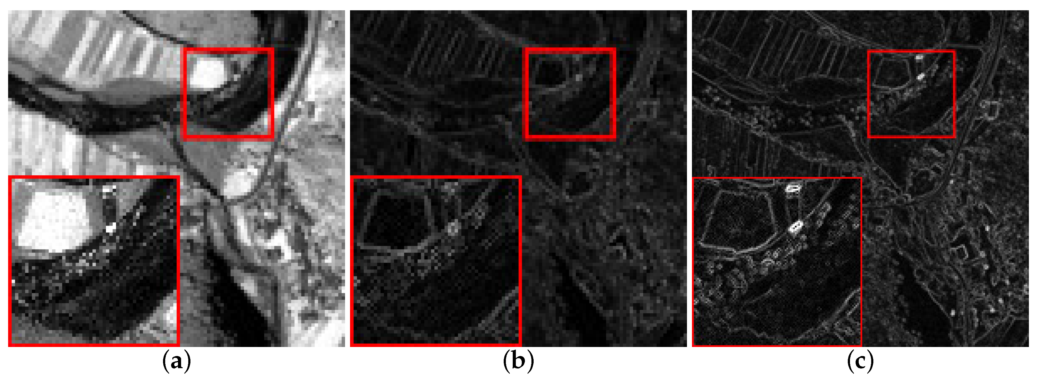
The gradient had a good description of the edge of the target, we used the data from the IKONOS satellite for gradient comparison Figure 1. Figure 1a is the original PAN image, Figure 1b is the gradient map of Figure 1a, and Figure 1c is the GSG map of Figure 1a. The small red box in the figure is the local image, and the large red box is the local enlarged image.

Figure 1.
Panchromatic image and gradient maps. (a) PAN; (b) IAIHS; (c) GIAIHS.
The figure shows that the edge of the original image is very obvious, which shows that the edge description of the original image had to be relatively close to the PAN image to better reflect the edge details of the pan image. From the GSG and original PAN images in Figure 1a, it is obvious that the two images had good similarities on the global edge of the image, especially in the relatively unobvious places, which can also show good edges and reflect the details. However, there is a serious blur phenomenon in the gradient image of Figure 1b, which had low similarity compared with the PAN image and could show less edge information. The comparative observation of Figure 1b,c shows that the GSG graph in Figure 1c had a significant increase in the extraction of edge information relative to Figure 1b.
3.3. Results
Because the model proposed in this paper is a two-stage PS model, to verify its effectiveness, an ablation experiment was preliminarily carried out.
For the proposed GIAIHS model, the IKONOS satellite contained a high-resolution PAN image (1 m resolution) and a low-resolution MS image (4 m resolution). IKONOS satellite data were selected for preliminary fusion analysis, and results are shown in Figure 2. The PAN image size of IKONOS satellite data was 400 × 400 pixels, and the MS image size was 100 × 100 pixels. The used MS image included four channels: red, blue, green, and near-infrared bands. Figure 2 shows that, through the effective fusion in the first stage compared with the IAIHS method, the quality of the fused image was greatly improved, especially for details such as boundaries.
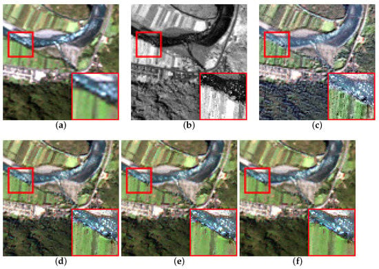
Figure 2.
Results of IKONOS satellite data fusion. (a) Upsampled MS. (b) PAN. (c) AIHS. (d) IAIHS. (e) First stage. (f) Second stage.
Analyzing the fusion results in Figure 2 showed that they were better in the first stage than those in the IAIHS method in terms of edge details; fusion results in the second stage were simultaneously better than those in the first stage in terms of edge details.
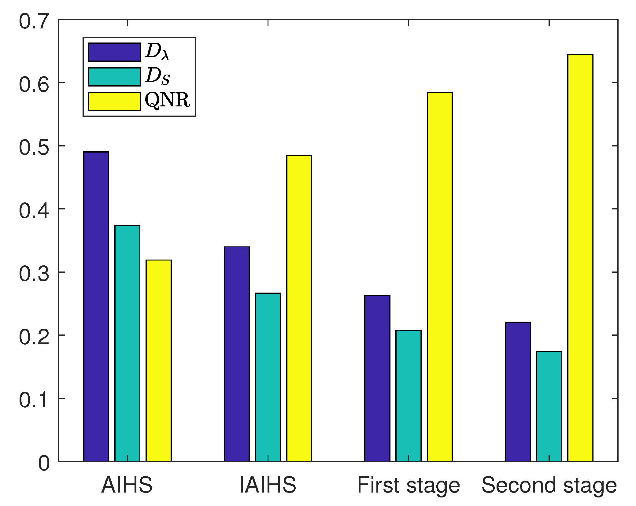
, and QNR are used for objective evaluation. can measure the spatial information of the fused image, and can measure the spectral information of the fused image, but their description of the overall information of the image is poor. The lower its value is, the better the spatial and spectral information of the fused image is. QNR can better measure the overall information of the fused image, and the higher the value is, the better the fusion effect. Figure 3 shows the comparison results of the three above indicators, where lower the purple and blue columns indicate better results, and yellow columns indicate better results. Figure 3 shows that the evaluation indices in the second stage had better results than those in the first stage. At the same time, the AIHS and IAIHS methods in the same CS method were compared to test the effectiveness of the model. The comparison showed hat the fusion results of the second stage of the GIAIHS model were better than those of the two methods regarding visual effect and evaluation index. To verify the feasibility of the model on the remaining satellite data, experiments with the MRA, VO, and ML methods were carried out.

Figure 3.
Comparative results of three indicators , , and QNR.
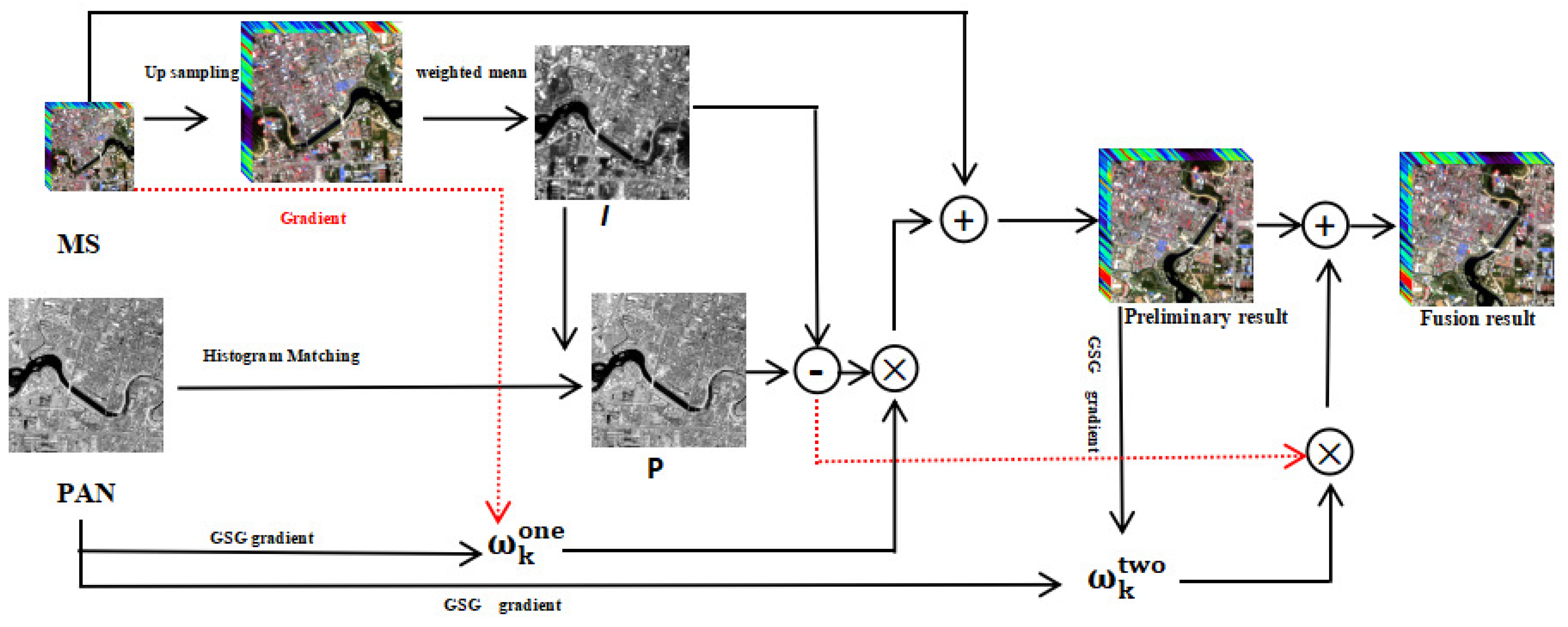
To better illustrate the model in this paper, the flow chart of the algorithm is given in Figure 4, where and are different weighting functions, as detailed in Algorithm 1.
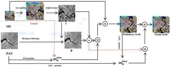
Figure 4.
GIAIHS flow chart.
4. Experiments and Analysis
4.1. Experimental Setup
All experiments were run on Windows 10 (64 bit) PC-Intel(R) Core (TM) i5-4210U CPU 2.40 GHz, 4 GB of RAM using MATLAB R2018b. We selected five different methods to compare with the GIAIHS method, namely, two CS methods (IAIHS and GSA), an MRA method (HPF), a VO method (RR), and a DL method (A-PNN). Due to the lack of corresponding high-spatial-resolution MS images in the experiment, the commonly used objective evaluation method is to downsample the fused image to the same size as the original MS image, and use the original MS image as the reference image for evaluation. In this paper, dimensionless global relative error of synthesis (ERGAS) [59], [60], relative average spectral error (RASE) [61], root mean squared error (RMSE), quality with no reference (QNR) [62], spectral distortion index , and spatial distortion index were used to evaluate the quality of the fused image.
The ERGAS index is a normalized dissimilarity index:
where is the ratio between the pixel sizes of PAN and MS, N is the total number of bands in the image, and refers to the mean value of K band. The lower the value of ERGAS was, the higher the correlation between fused and MS images, that is, the better the quality of the fused image.
The Q4 index was derived from index, and formula is as follows:
where and represent the pixel spectral vector of MS and fused images, and refers to the average value of the whole image, which is usually divided into block.
The RASE index is defined as
where represents the k band of the fused image, and represents the k band of the MS image, which is used to calculate the global spectral quality of the fused image. The smaller the value of RASE is, the better the quality of the fused image.
The RMSE index is defined as
When I = J, RMSE reaches the ideal value of zero. It is used to calculate the average difference between fused and MS images. The smaller the value of RMSE is, the better the quality of the fused image.
The assumption of the QNR index is that the similarity between each MS band and PAN should remain unchanged before and after fusion. Before calculating QNR, spectral distortion index and spatial distortion index need to be calculated.
Spectral distortion index is estimated by
the closer the value of is to 0, the greater the spectral distortion of the fused image and the better the quality of the fused image are.
Spatial distortion index is estimated by
where is the image with the same size from the PAN image downsampling to MS image. The closer the value of is to 0, the greater the spatial distortion of the fused image and the better the quality of the fused image are.
The QNR index is estimated by
it is obtained by weighting and by and ; the higher the QNR value is, the better the quality of the fused image. When both and are 0, QNR theoretically reaches the optimal value of 1.
4.2. Datasets
To further verify the effectiveness of the proposed model, experimental comparison and analysis were carried out on QuickBird, Gaofen-1, and Worldview-4 satellite data. The QuickBird satellite contains a high-resolution PAN image (0.7 m resolution) and a low-resolution MS image (2.8-m resolution). The Gaofen-1 satellite contains a high-resolution PAN image (2-m resolution) and a low-resolution MS image (8-m resolution). The Worldview-4 satellite contains a high-resolution PAN image (0.31-m resolution) and a low-resolution MS image (1.24-m resolution). The PAN image size used by QuickBird satellite data is 800 × 800 pixels, and the MS image size is 200 × 200 pixels. The PAN image size of Gaofen-1 satellite data is 1024 × 1024 pixels, and the MS image size is 256 × 256 pixels. In worldview-4 satellite data, the PAN image size is 1024 × 1024 pixels, and the MS image size is 256 × 256 pixels. The MS images used include four channels: red, blue, green, and near-infrared. The image was corrected for radiation and sensor distortion, and the acquisition effect was eliminated. In addition, collected satellite images were corrected for viewing angle and ground effect so that they can be superimposed on the map. In addition, orthophoto correction is carried out to eliminate the perspective effect on the ground. The best input format of data is the TIF format.
4.3. Experiments and Analysis
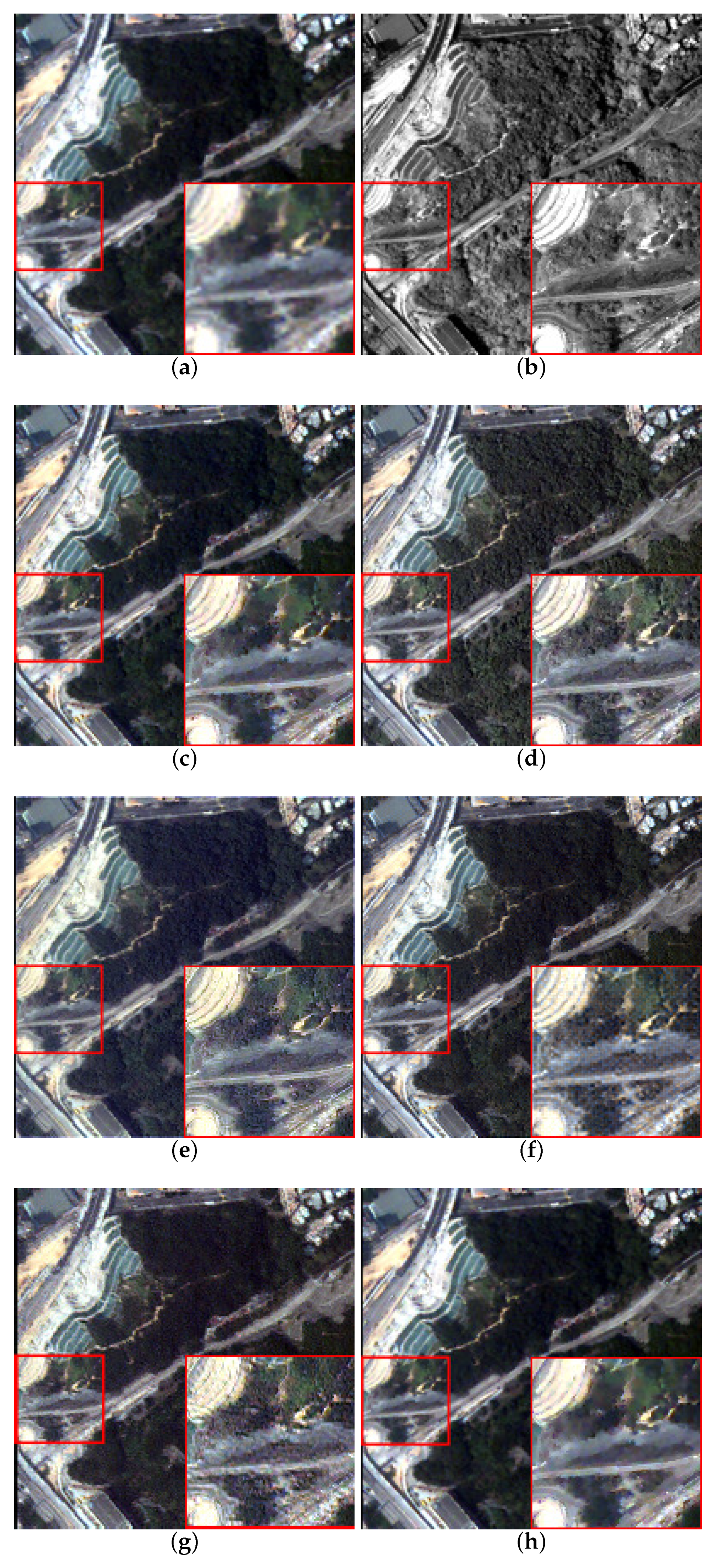
The subjective visual comparison results of three different satellite data fusion are shown in Figure 5, Figure 6 and Figure 7, and a local map is also given for further observation. The red block diagram on the center is the selected local terrain, and the lower right corner is the local enlarged view corresponding to the center side.
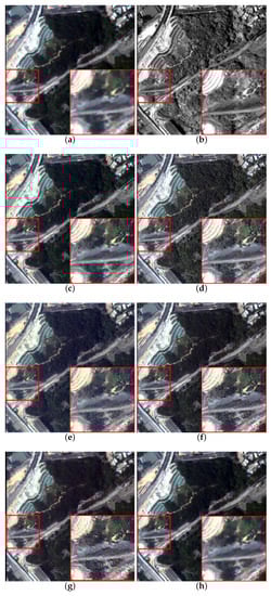
Figure 5.
Fusion results of six different PS fusion methods in QuickBird data fusion. (a) Upsampled MS. (b) PAN. (c) IAIHS. (d) GSA. (e) HPF. (f) RR. (g) A-PNN. (h) GIAIHS.

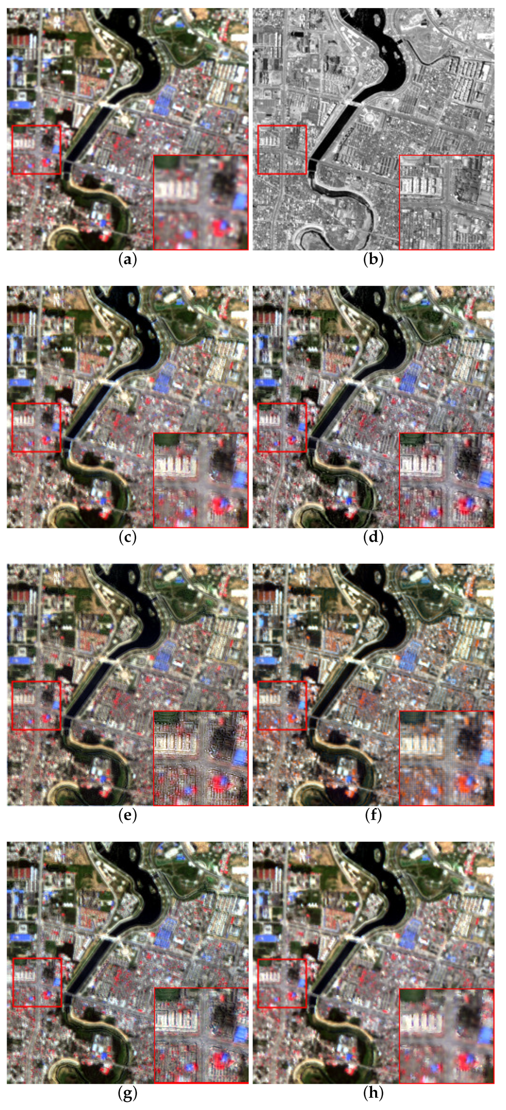
Figure 6.
Fusion results of six different PS fusion methods in Gaofen-1 data fusion. (a) Upsampled MS. (b) PAN. (c) IAIHS. (d) GSA. (e) HPF. (f) RR. (g) A-PNN. (h) GIAIHS.

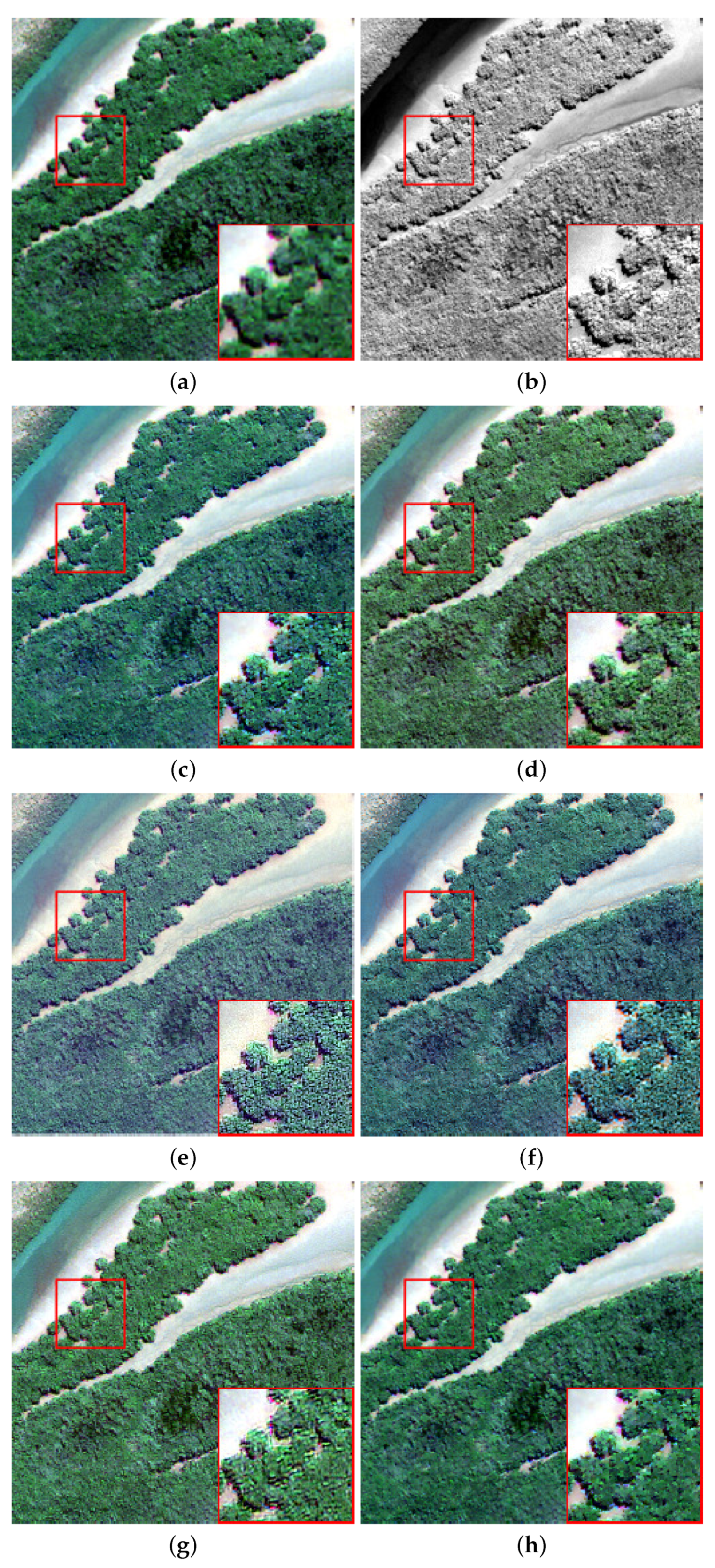
Figure 7.
Fusion results of six different PS fusion methods in Worldview-4 data. (a) Upsampled MS. (b) PAN. (c) IAIHS. (d) GSA. (e) HPF. (f) RR. (g) A-PNN. (h) GIAIHS.
Because the resolution of the MS image used in this paper was inconsistent with that of the PAN image, the resolution of the MS image needed to be upsampled to be consistent with that of the PAN image, and then fused by PS method. The resolution of the fused image was consistent with that of the PAN image. In the process of visual analysis, to better reflect the advantages of this method, the upsampled image of MS image was compared with other fused images, which could better reflect the differences of various methods in quasitube vision. In quantitative analysis, there was a lack of high-resolution reference images. According to Wald’s protocol [63], the fused image was downsampled to the same size as the original MS image, and the downsampled fused image is quantitatively analyzed with MS image.
These three sets of satellite data were chosen for the following reason: the terrain shown in QuickBird satellite data includes urban roads, rural areas, and a large number of forestry areas. The terrain shown in the Gaofen-1 satellite data is mainly waterways with a large number of urban areas beside it, which is complex. The terrain displayed in Worldview-4 satellite data is mainly forestry, which can highlight the details.
Remote-sensing images obtained by QuickBird satellite include rural and forestry areas. Fusion results are shown in Figure 5. PS results obtained by the HPF and RR methods lost a lot of spectral information, resulting in overall color changing. GSA and IAIHS showed that the visual effect of these two methods is too bright in some areas. For example, the color of the boundary in the enlarged image (Figure 5c,d) was significantly different from the actual color. Fusion results obtained by the A-PNN method had similar visual effects. It can be seen from the enlarged image that the method proposed in this paper can obtain clearer PS results. The objective evaluation results of rural areas are shown in Table 1. The best performance is shown in bold.

Table 1.
Experiment with six PS methods on QuickBird satellite data.
In the city image taken by Gaofen-1 satellite, the comparison diagram between this method and five other methods is given in Figure 6, which shows that the description of the outline of urban areas by the IAIHS and RR methods was not clear enough, and the roofs of some buildings turned gray. At the same time, details of the house showed that the GSA method had serious spatial distortion. The outline produced by the HPF method was too enhanced, and the image color was too bright, which produced artifacts. However, the middle road of the A-PNN method was close to white, and there is no strong color display. This method preserves a lot of spectral information in the experiment and fully uses the spatial information of PAN images. The objective evaluation of the city image is shown in Table 2. The best performance is shown in bold.
Table 2.
Experiment with six PS methods on Gaofen-1 satellite data.
Figure 7 is a forest vegetation image taken by the WV-4 satellite. The fused image obtained by the HPF method was severely distorted, and the color of the trees tended to be blue. This method loses a lot of spectral information when balancing spatial and spectral information. In addition, spectral information of the GSA method was distorted due to the mismatch of spectral ranges. The spectra of the IAIHS and RR methods were relatively well-preserved, but some spatial details were lost. Spectral information of fusion results obtained by the A-PNN method was good, but some fuzzy effects could be found from the vegetation region. The method in this paper can fully use spectral information in MS images and spatial information in PAN images. The objective evaluation of forest vegetation is shown in Table 3. The best performance is shown in bold.
Table 3.
Experiment with six PS methods on WorldView-4 satellite data.
Table 1 shows the comparison result of QuickBird satellite data. Table 1 shows that the GIAIHS method showed great improvement compared with other methods. For the RASE index, the GIAIHS method improved by approximately 26% compared with the GSA method. For the ERGAS index, the GIAIHS method improved by approximately 19% compared with the RR method. For Q4, GIAIHS method improved by approximately 20% over the A-PNN method. For , GIAIHS method improved by approximately 35% over IAIHS method.
Table 2 shows the comparison result of Gaofen-1 satellite data. Table 2 shows that, for the RASE index, the GIAIHS method improved by approximately 50% compared with the GSA method. For the ERGAS index, the GIAIHS method improved by approximately 29% compared with the RR method. For Q4, GIAIHS method improved by approximately 7% over A-PNN method. For , GIAIHS method improved by approximately 48% over IAIHS method.
Table 3 shows the comparison result of Worldview-4 satellite data. Table 3 shows that, for the RASE index, the GIAIHS method improved by approximately 26% compared with the GSA method. For the ERGAS index, the GIAIHS method improved by approximately 29% compared with the RR method. For Q4, GIAIHS method improved by approximately 8% over A-PNN method. For , GIAIHS method improved by approximately 60% over IAIHS method.
Table 1 shows that, for , the GIAIHS method differed from the A-PNN method by only approximately 0.01 in the QuickBird data, but GIAIHS was greatly improved compared with other methods. At the same time, for the QNR index, GIAIHS method improved by approximately 12% over A-PNN method. Table 2 shows that, for , the GIAIHS and A-PNN methods achieved the same performance level in Gaofen-1 data; for the QNR index, GIAIHS method improved by approximately 16% over A-PNN method. Table 3 shows that, for , the GIAIHS method differed from the A-PNN method by only approximately 0.02 in Worldview-4 data; for the QNR index, GIAIHS method improved by approximately 4% over A-PNN method.
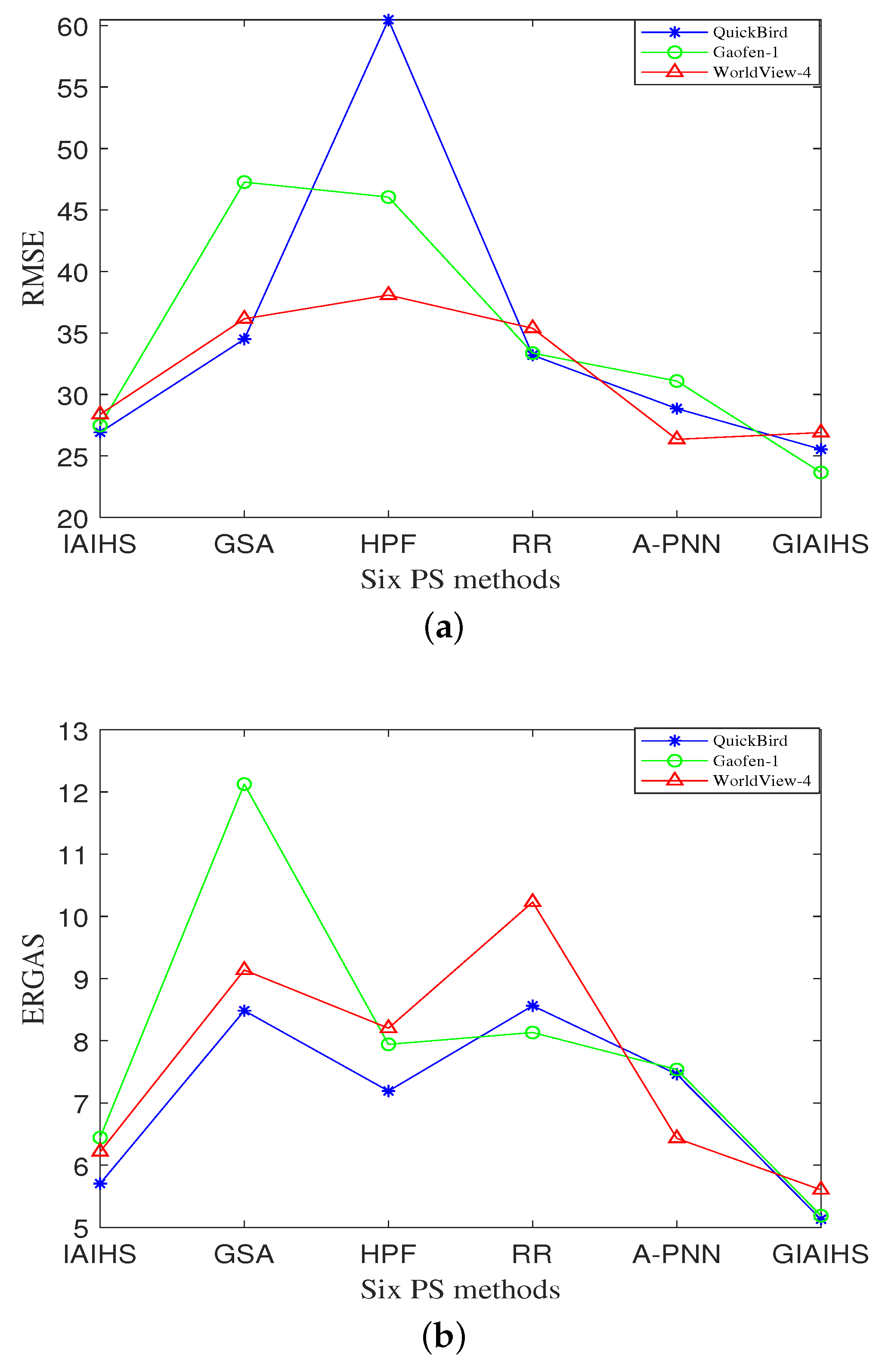
Figure 8 shows the RMSE and ERGAS evaluation results of the six methods for three different satellites’ data. The method had good stability, which was maintained in the evaluation of three different satellite data in this paper. RMSE evaluation results and the fluctuation of ERGAS displayed in Figure 8 show that the method had good robustness. This method is highly competitive with the rest of the methods. In addition, from a statistical point of view, the method proposed in this paper is better than other methods.
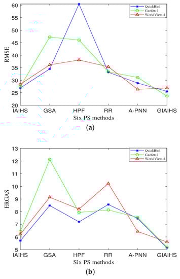
Figure 8.
RMSE and ERGAS evaluation results of GIAIHS method and five other methods in three groups of different satellite data of QuickBird, Gaofen-1 and WorldView-4. (a) RMSE results. (b) ERGAS results.
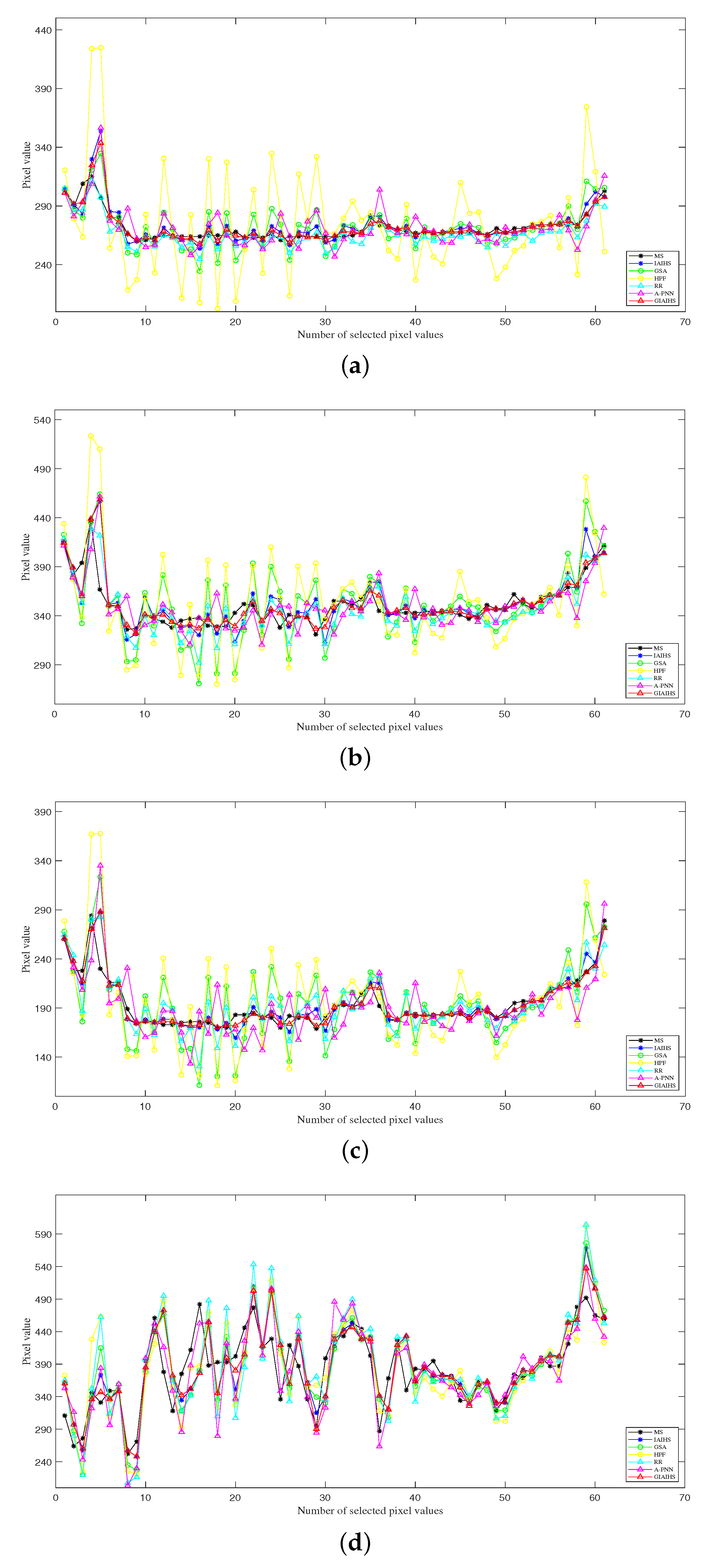
To better illustrate the spectral effect of the method in this paper, QB satellite data results were selected for comparative analysis. Because the resolution of the fused image was different from that of the original MS image, the downsampling of the fused image was consistent with that of the original MS image for comparative analysis. Figure 9 shows the comparative analysis of the original MS image and the results of six PS methods, in which the x axis represents the 61 selected pixels (because image resolution was 256 × 256, 61 pixels were selected in the middle part of the image), and the y axis represents the pixel value corresponding to the pixels. The fusion experiment in this paper was carried out in four bands. Figure 9a shows the comparison results of pixels selected by different methods in the R band, Figure 9b shows the comparison results of pixels selected in G band, Figure 9c shows the comparison results of pixels selected in B band, and Figure 9d shows the comparison results of pixels selected in NIR band.
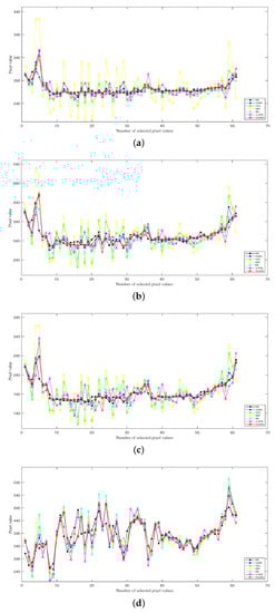
Figure 9.
Results of spectral comparison and analysis of QuickBird satellite data. (a) R band. (b) G band. (c) B band. (d) NIR band.
The black line segment in Figure 9 is marked with 61 pixel values corresponding to the original MS image, and the six other line segments are pixel values corresponding to the IAIHS, GSA, HPF, RR, A-PNN, and GIAIHS methods, respectively. Figure 9a shows that the obtained results by the GIAIHS method were very close to the results of the original MS image, followed by A-PNN results and RR results. In Figure 9b, some pixel values of GIAIHS method are consistent with those of the original MS. There was not much difference between the GSA and HPF methods, but they are still very different from the pixel value curve of MS. Although the A-PNN method was better than the GIAIHS method, there were still some differences. Figure 9c shows that the results of the RR method and A-PNN were not very good. There was large deviation in some points, which was better than IAIHS. Only a few points deviated from the Ms results, while GIAIHS almost had a small gap with MS. The above analysis proves that GIAIHS had good performance in the spectrum.
In general, the GIAIHS method not only outperformed state-of-the-art methods, but also had some competitiveness with the DL method of A-PNN method, which also shows that the objective evaluation of the GIAIHS method is well consistent with the subjective evaluation.
5. Conclusions
In this paper, we proposed a two-stage fusion method for PS by combining the CS method with the variational idea. We used a GSG that could more fully reflect the image texture and edge information for the construction of the weight function, and further refine the fusion results to improve the PS results effectively. The GIAIHS method significantly improves the quality of the fused images, and also improves the generalization ability of the method to data from different satellites.
In performing PS, the main objective is to maintain the integrity of spectral information of MS images and spatial information of PAN images. First, we chose GSG as the weight function to fully extract the information of the image. Second, for obtained results by direct fusion, we used IKONOS data to analyze them, and performed a two-stage thinning process. Results showed that it was necessary to perform this thinning process. Experimenting on different datasets demonstrated that our proposed two-stage PS method is effective in obtaining better-quality fused images compared to other methods. Since our proposed method is required to extract more detailed information from the images, better results could be obtained when processing higher dimensional as well as more complex images. The method is better at processing spectral and spatially informative images, while it can effectively capture rich features from dense buildings and dense vegetation, which helps in generating satisfactory high-quality fusion images.
The method proposed in this paper combines the classical CS and variational methods. Experimental results showed that the idea proposed in this paper is effective. The advantage of this model is that it produced good experimental results for different satellite data from both subjective vision and quantitative indicators, and had strong generalization ability. The disadvantage is that the proposed model had more parameters. In the next step, it was changed into an adaptive parameter model. For a future research direction, because the methods that could describe image features in detail are very limited, and remote-sensing image PS based on deep learning have developed rapidly in recent years, future classical methods can be integrated into deep learning and models driven for PS. Next, we also aim to apply the plug-and-play idea [64] to the classical method. Since the MS images used in this paper had four bands, more bands of images will be PS-fused.
Author Contributions
Conceptualization, Y.W., G.L., R.Z. and J.L.; methodology, Y.W.; software, Y.W.; validation, Y.W.; investigation, Y.W. and G.L.; resources, Y.W., G.L. and R.Z.; data curation, Y.W. and J.L.; writing original draft preparation, Y.W.; visualization, Y.W. All authors have read and agreed to the published version of the manuscript.
Funding
This work was supported by the National Natural Science Foundation of China under grant 62061040, in part by the project funded by the Ningxia Natural Science Foundation under grants 2018AAC03014 and 2021AAC03045, and in part by the Key Research and Development Plan in Ningxia District under grant 2019BEG03056.
Institutional Review Board Statement
Not applicable.
Informed Consent Statement
Not applicable.
Data Availability Statement
Not applicable.
Conflicts of Interest
The authors declare no conflict of interest.
References
- Shah, V.P.; Younan, N.H.; King, R.L. An efficient pansharpening method via a combined adaptive PCA approach and contourlets. IEEE Trans. Geosci. Remote Sens. 2008, 46, 1323–1335. [Google Scholar] [CrossRef]
- Aiazzi, B.; Baronti, S.; Selva, M. Improving component substitution pansharpening through multivariate regression of MS + Pan data. IEEE Trans. Geosci. Remote Sens. 2007, 45, 3230–3239. [Google Scholar] [CrossRef]
- Tu, T.M.; Su, S.C. A new look at IHS like image fusion methods. Inform. Fus. 2001, 2, 177–186. [Google Scholar] [CrossRef]
- Kang, X.; Li, S.; Benediktsson, J.A. Pansharpening with matting model. IEEE Trans. Geosci. Remote Sens. 2014, 52, 5088–5099. [Google Scholar] [CrossRef]
- Rahmani, S.; Strait, M.; Merkurjev, D.; Merkurjev, D. An adaptive IHS pansharpening method. IEEE Geosci. Remote Sens. Lett. 2010, 52, 746–750. [Google Scholar] [CrossRef] [Green Version]
- Leung, Y.; Liu, J.M.; Zhang, J. An improved adaptive intensity hue saturation method for the fusion of remote sensing images. IEEE Geosci. Remote Sens. Lett. 2013, 11, 985–989. [Google Scholar] [CrossRef]
- Chen, Y.X.; Zhang, G.X. A pansharpening method based on evolutionary optimization and IHS transformation. Math. Probl. Eng. 2017, 2017, 8269078. [Google Scholar] [CrossRef] [Green Version]
- Chen, Y.X.; Liu, C.; Zhou, A.; Zhang, G.X. MIHS: A multiobjective pan sharpening method for remote sensing images. In Proceedings of the IEEE Congress on Evolutionary Computation, Wellington, New Zealand, 10–13 June 2019; pp. 1068–1073. [Google Scholar]
- Garzelli, A.; Nencini, F.; Capobianco, L. Optimal MMSE pansharpening of very high resolution multispectral images. IEEE Trans. Geosci. Remote Sens. 2008, 46, 228–236. [Google Scholar] [CrossRef]
- Vivone, G. Robust band-dependent spatial-detail approaches for panchromatic sharpening. IEEE Trans. Geosci. Remote Sens. 2019, 57, 6421–6433. [Google Scholar] [CrossRef]
- Choi, J.; Yu, K.; Kim, Y. A new adaptive component substitution based satellite image fusion by using partial replacement. IEEE Trans. Geosci. Remote Sens. 2010, 49, 295–309. [Google Scholar] [CrossRef]
- Shahdoosti, H.R.; Javaheri, N. Pansharpening of clustered MS and PAN images considering mixed pixels. IEEE Geosci. Remote Sens. Lett. 2017, 14, 826–830. [Google Scholar] [CrossRef]
- Zhao, X.L. Image fusion based on IHS transform and principal component analysis transform. In Proceedings of the International Conference on Computer Technology Electronics and Communication, Allahabad, India, 17–19 September 2010; pp. 304–307. [Google Scholar]
- Alparone, L.; Baronti, S.; Aiazzi, B.; Garzelli, A. Spatial methods for multi-spectral pansharpening: Multi-resolution analysis demystified. IEEE Trans. Geosci. Remote Sens. 2016, 54, 2563–2576. [Google Scholar] [CrossRef]
- Wang, Z.J.; Ziou, D.; Armenakis, C.; Li, D.R.; Li, Q. A comparative analysis of image fusion methods. IEEE Trans. Geosci. Remote Sens. 2017, 43, 1391–1402. [Google Scholar] [CrossRef]
- Restaino, R.; Mura, M.D.; Vivone, G.; Chanussot, J. Context adaptive pansharpening based on image segmentation. IEEE Trans. Geosci. Remote Sens. 2016, 55, 753–766. [Google Scholar] [CrossRef] [Green Version]
- Vivone, G.; Marano, S.; Chanussot, J. Pansharpening: Context-based generalized laplacian pyramids by robust regression. IEEE Trans. Geosci. Remote Sens. 2020, 58, 6152–6167. [Google Scholar] [CrossRef]
- Restaino, R.; Vivone, G.; Dalla, M.M.; Chanussot, J. Fusion of multispectral and panchromatic images based on morphological operators. Photogramm. Eng. Remote Sens. 2016, 25, 2882–2895. [Google Scholar] [CrossRef] [Green Version]
- Aiazzi, B. MTF tailored multiscale fusion of high resolution ms and pan imagery. Photogramm. Eng. Remote Sens. 2015, 72, 591–596. [Google Scholar] [CrossRef]
- Ballester, C.; Caselle, S.V.; Igual, L.; Verdera, J.; Rougé, B. A variational model for P+XS Image fusion. Int. J. Comput. Vis. 2006, 69, 43–58. [Google Scholar] [CrossRef]
- Palsson, F.; Ulfarsson, M.O.; Sveinsson, J.R. Model based reduced rank pansharpening. IEEE Geosci. Remote Sens. Lett. 2020, 17, 656–660. [Google Scholar] [CrossRef]
- Vega, M.; Mateos, J.; Molina, R.; Katsaggelos, A.K. Super resolution of multispectral images using TV image models. Knowl.-Based Intell. Inf. Eng. Syst. 2008, 19, 408–415. [Google Scholar]
- Duran, J.; Buades, A.; Coll, B.; Sbert, C. A nonlocal variational model for pansharpening image fusion. SIAM J. Imaging Sci. 2014, 7, 761–796. [Google Scholar] [CrossRef]
- Li, S.T.; Dian, R.W.; Fang, L.Y.; Bioucas, J.M. Fusing hyperspectral and multispectral images via coupled sparse tensor factorization. IEEE Trans. Image Process. 2018, 27, 4118–4130. [Google Scholar] [CrossRef] [PubMed]
- Wang, K.; Wang, Y.; Zhao, X.L.; Meng, D.Y.; Xu, Z.B. Hyperspectral and multisectral image fusion via nonlocal low-rank tensor decomposition and spectral unmixing. IEEE Geosci. Remote Sens. 2020, 58, 7654–7671. [Google Scholar] [CrossRef]
- Andrea, G. A review of image fusion algorithms based on the super resolution paradigm. Remote Sens. 2016, 8, 797. [Google Scholar]
- Tian, X.; Chen, Y.; Yang, C.; Zhang, M.; Ma, J. A variational pansharpening method based on gradient sparse representation. IEEE Signal Process. Lett. 2020, 27, 1180–1184. [Google Scholar] [CrossRef]
- Fu, X.; Lin, Z.; Huang, Y.; Ding, X. A variational pansharpening with local gradient constraints. In Proceedings of the IEEE/CVF Conference on Computer Vision and Pattern Recognition, Long Beach, CA, USA, 16–20 June 2019; pp. 10265–10274. [Google Scholar]
- Deng, L.J.; Vivone, G.; Guo, W.; Dalla Mura, M.; Chanussot, J. A variational pansharpening approach based on reproducible kernel Hilbert space and heaviside function. IEEE Trans. Image Process. 2018, 27, 4330–4344. [Google Scholar] [CrossRef]
- Zhang, Z.Y.; Huang, T.Z.; Deng, L.J.; Huang, J.; Zhao, X.L.; Zheng, C.C. A framelet-based iterative pan-sharpening approach. Remote Sens. 2018, 10, 622. [Google Scholar] [CrossRef] [Green Version]
- Xu, T.; Huang, T.Z.; Deng, L.J.; Zhao, X.L.; Huang, J. Hyperspectral image superresolution using unidirectional total variation with tucker decomposition. IEEE J. Sel. Top. Appl. Earth Obs. Remote Sens. 2020, 13, 4381–4398. [Google Scholar] [CrossRef]
- Deng, L.J.; Feng, M.; Tai, X.C. The fusion of panchromatic and multispectral remote sensing images via tensor-based sparse modeling and hyper-Laplacian prior. Inf. Fusion 2019, 52, 76–89. [Google Scholar] [CrossRef]
- Huang, W.; Xiao, L.; Wei, Z.; Liu, H.; Tang, S. A new pan sharpening method with deep neural networks. IEEE Geosci. Remote Sens. Lett. 2015, 12, 1037–1041. [Google Scholar] [CrossRef]
- Masi, G.; Cozzolino, D.; Verdoliva, L.; Scarpa, G. Pansharpening by convolutional neural networks. Remote Sens. 2016, 8, 594. [Google Scholar] [CrossRef] [Green Version]
- Scarpa, G.; Vitale, S.; Cozzolino, D. Target-adaptive CNN-based pansharpening. IEEE Trans. Geosci. Remote Sens. 2018, 56, 5443–5457. [Google Scholar] [CrossRef] [Green Version]
- Wei, Y.C.; Yuan, Q.Q.; Shen, H.F.; Zhang, L.P. Boosting the accuracy of multispectral image pansharpening by learning a deep residual network. IEEE Geosci. Remote Sens. Lett. 2017, 14, 1795–1799. [Google Scholar] [CrossRef] [Green Version]
- Yang, Y.; Tu, W.; Huang, S.; Lu, H. PCDRN: Progressive cascade deep residual network for pansharpening. Remote Sens. 2020, 12, 676. [Google Scholar] [CrossRef] [Green Version]
- Ma, J.; Yu, W.; Chen, C.; Liang, P.; Jiang, J. Pan-GAN: An unsupervised pansharpening method for remote sensing image fusion. Inf. Fusion 2020, 62, 110–120. [Google Scholar] [CrossRef]
- Fu, X.; Wang, W.; Huang, Y.; Ding, X.; Paisley, J. Deep multiscale detail networks for multiband spectral image sharpening. IEEE Trans. Neural Netw. Learn. Syst. 2020, 32, 2090–2104. [Google Scholar] [CrossRef]
- Deng, L.J.; Vivone, G.; Jin, C.; Chanussot, J. Detail injection-based deep convolutional neural networks for pansharpening. IEEE Trans. Geosci. Remote Sens. 2021, 59, 6995–7010. [Google Scholar] [CrossRef]
- Jin, C.; Deng, L.J.; Huang, T.Z.; Vivone, G. Laplacian pyramid networks: A new approach for multispectral pansharpening. Inf. Fusion 2022, 78, 158–170. [Google Scholar] [CrossRef]
- Cao, X.; Fu, X.; Xu, C.; Meng, D. Deep spatial-spectral global reasoning network for hyperspectral image denoising. IEEE Trans. Geosci. Remote Sens. 2021, 60, 1–14. [Google Scholar] [CrossRef]
- Liu, P.; Xiao, L. A nonconvex pansharpening model with spatial and spectral gradient difference-induced nonconvex sparsity priors. IEEE Trans. Geosci. Remote Sens. 2021, 60, 1–15. [Google Scholar] [CrossRef]
- Xiang, Z.; Xiao, L.; Liao, W.; Philips, W. MC-JAFN: Multilevel contexts-based joint attentive fusion network for pansharpening. IEEE Geosci. Remote Sens. Lett. 2021, 19, 1–5. [Google Scholar] [CrossRef]
- Li, K.; Zhang, W.; Tian, X.; Ma, J.; Zhou, H.; Wang, Z. Variation-Net: Interpretable variation-inspired deep network for pansharpening. In Proceedings of the 2021 IEEE International Conference on Multimedia and Expo (ICME), Shenzhen, China, 5–9 July 2021; pp. 1–6. [Google Scholar]
- Guo, P.; Zhuang, P.; Guo, Y. Bayesian pan-sharpening with multiorder gradient-based deep network constraints. IEEE J. Sel. Top. Appl. Earth Obs. Remote Sens. 2020, 13, 950–962. [Google Scholar] [CrossRef]
- Lei, D.; Huang, Y.; Zhang, L.; Li, W. Multibranch feature extraction and feature multiplexing network for pansharpening. IEEE Trans. Geosci. Remote Sens. 2021, 59, 2231–2244. [Google Scholar] [CrossRef]
- Zhang, H.; Ma, J. GTP-PNet: A residual learning network based on gradient transformation prior for pansharpening. ISPRS J. Photogramm. Remote Sens. 2021, 172, 223–239. [Google Scholar] [CrossRef]
- Hu, J.; Du, C.; Fan, S. Two-stage pansharpening based on multi-level detail injection network. IEEE Access. 2020, 8, 156442–156455. [Google Scholar] [CrossRef]
- Wu, Y.; Huang, M.; Li, Y.; Feng, S.; Wu, D. A distributed fusion framework of multispectral and panchromatic images based on residual network. Remote Sens. 2021, 13, 2556. [Google Scholar] [CrossRef]
- Vitale, S.; Scarpa, G. A detail-preserving cross-scale learning strategy for CNN-based pansharpening. Remote Sens. 2020, 12, 348. [Google Scholar] [CrossRef] [Green Version]
- Wang, W.; Zhou, Z.; Liu, H.; Xie, G. MSDRN: Pansharpening of multispectral images via multi-scale deep residual network. Remote Sens. 2021, 13, 1200. [Google Scholar] [CrossRef]
- Naushad, R.; Kaur, T.; Ghaderpour, E. Deep transfer learning for land use and land cover classification: A comparative study. Sensors 2021, 21, 8083. [Google Scholar] [CrossRef]
- Xu, H.; Le, Z.; Huang, J.; Ma, J. A cross direction and progressive network for pansharpening. Remote Sens. 2021, 13, 3045. [Google Scholar] [CrossRef]
- Palsson, F.; Sveinsson, J.R.; Ulfarsson, M.O. A new pansharpening algorithm based on total variation. IEEE Geosci. Remote Sens Lett. 2013, 11, 318–322. [Google Scholar] [CrossRef]
- Osher, S. Nonlocal operators with applications in imaging. Multiscale Model. Simul. 2008, 7, 1005–1028. [Google Scholar]
- Zhang, R. Research of Global Sparse Gradient Based Image Processing Methods. Ph.D. Dissertation, Xidian University, Xi’an, China, 2017. [Google Scholar]
- Yang, X.M.; Jian, L.H.; Yan, B.Y.; Liu, K.; Zhang, L.; Liu, Y.G. A sparse representation based pansharpening method. Future Gener. Comput. Syst. 2018, 88, 385–399. [Google Scholar] [CrossRef]
- Alparone, L.; Baronti, S.; Garzelli, A.; Nencini, F. A global quality measurement of pansharpened multispectral imagery. IEEE Geosci. Remote Sens. Lett. 2004, 1, 313–317. [Google Scholar] [CrossRef]
- Pushparaj, J.; Hegde, A. Evaluation of pansharpening methods for spatial and spectral quality. Appl. Geomat. 2008, 9, 1–12. [Google Scholar] [CrossRef]
- Choi, M. A new intensity hue saturation fusion approach to image fusion with a tradeoff parameter. IEEE Trans. Geosci. Remote Sens. 2006, 6, 1672–1682. [Google Scholar] [CrossRef] [Green Version]
- Alparone, L.; Aiazzi, B.; Baront, I.S.; Garzelli, A.; Nencini, F.; Selva, M. Multispectral and panchromatic data fusion assessment without reference. Photogramm. Eng. Remote Sens. 2008, 74, 193–200. [Google Scholar] [CrossRef] [Green Version]
- Wald, L.; Ranchin, T.; Mangolini, M. Fusion of satellite images of different spatial resolutions: Assessing the quality of resulting images. Photogramm. Eng. Remote Sens. 1997, 63, 691–699. [Google Scholar]
- Zhang, K.; Li, Y.; Zuo, W. Plug-and-Play image restoration with deep denoiser prior. IEEE Trans. Pattern Anal. Mach. Intell. 2021, 99, 1. [Google Scholar] [CrossRef]

Publisher’s Note: MDPI stays neutral with regard to jurisdictional claims in published maps and institutional affiliations. |
© 2022 by the authors. Licensee MDPI, Basel, Switzerland. This article is an open access article distributed under the terms and conditions of the Creative Commons Attribution (CC BY) license (https://creativecommons.org/licenses/by/4.0/).