An Inverse Method for Drop Size Distribution Retrieval from Polarimetric Radar at Attenuating Frequency

Abstract

A method that formulates the retrieval of drop size distribution (DSD) parameters from polarimetric radar variables at attenuating frequency as the solution of an inverse problem is presented. The DSD in each radar bin is represented by a normalized Gamma distribution defined by three parameters ($D_m,N_0^{*},\mu$). The direct problem that describes polarimetric radar observables—scattering and propagation terms—and their dependency on DSD parameters is analyzed based on T-matrix scattering simulations. The inverse algorithm and its application to the DSD retrieval are then presented. The inverse method is applied to an African Monsoon Multidisciplinary Analysis (AMMA) field campaign that deployed an X-band dual-polarization Doppler radar and optical disdrometers in Benin, West Africa, in 2006 and 2007. The dataset is composed of X-band polarimetric radar PPIs and disdrometer data for 15 organized convective systems observed in 2006. A priori information on DSD parameters (benchmark method) is derived from the polarimetric radar observables by applying power law relationships. The proposed retrieval method of DSD parameters leads to the following results as compared to the benchmark: (i) we found a better spatial consistency of the retrieved parameters, (ii) the reconstructed polarimetric radar observables are closer to the observations, (iii) The validation with disdrometer data confirms an improved estimation of the DSD parameters.

1. Introduction

Rainfall estimation has greatly benefitted from the progress of weather radar and the development of dual-polarization methods. A whole branch of weather radar research has been devoted to rain or cloud drop size distributions (DSD), with two purposes: (i) characterizing DSD and its variability as a source of uncertainty in radar estimation of rainfall [1,2,3,4,5,6] and (ii) deriving information on the DSD from the radar measurements itself [7,8,9]. The determination of the DSD over various spatial and temporal scales is interesting for a range of scientific applications, including: rain rate estimation, rain erosivity [10], satellite and radar remote sensing studies [11,12], rain microphysics, cloud modeling, among others. Most of the early work on the DSD was based on disdrometers and mainly focused on investigating if some standard form of DSD could be defined [13]. It is commonly accepted that rainfall DSD can be represented by a Gamma law governed by three parameters characterizing: the number of drops, the characteristic diameter, and the distribution shape [14]; other laws such as lognormal or four-parameters extended gamma have also been proposed, but are less commonly used. Many studies have been devoted to analyzing how the DSD parameters vary with rain bulk variables (rain rate, radar reflectivity factor, liquid water content, median-volume diameter) and to finding expressions for the DSD function and parameters that reduce the variability [14,15]. A well-adapted solution consists in normalizing the DSD and the drop diameters by one or two integral moments of the DSD [13,14] among others).

Disdrometers provide only local information on the DSD and no information on its spatial variability unless an extensive network of disdrometers is used. Radar polarimetry has led to significant progress in rainfall characterization, helping to document both spatial and temporal variability. A polarimetric radar provides several variables useful to characterize rainfall (see Section 3.1). The retrieval of DSDs was initially proposed as a means to improve rainfall estimation from polarimetric variables [16]. The authors of [16,17] proposed the $\beta$-method, improved in [18], to retrieve the parameters of a DSD gamma distribution. The authors of [19,20] developed the constrained gamma method to derive relations expressing the DSD parameters as functions of reflectivity and differential reflectivity. According to [21,22], the constrained gamma method performs better than the $\beta$-method. The authors of [23] developed a method applicable to a double-moment normalized DSD, defined by two parameters. The authors of [8] tested retrievals of DSD based on empirical relationships applied to radar polarimetric variables in Africa. The authors of [24] used a tree-based genetic program to retrieve the parameters of a gamma DSD from reflectivity and differential reflectivity. The authors of [25] proposed a Bayesian approach with DSD parameters as state variables to estimate rainfall rate from S-band polarimetric radar. The authors of [26] formulated the retrieval of DSD parameters from S-band polarimetric radar variables as an inverse problem.

The studies above do not explicitly account for radar attenuation by rain. For X-band radars, the reflectivity variables must be corrected for attenuation to avoid underestimation of the DSD parameters. The authors of [27,28,29] adapted the self-consistent method proposed by [30] for attenuation correction of X-band data. The authors of [18] also used a self-consistency method. The authors of [23] proposed a variation on the ZPHI algorithm [31]. In most studies, a relationship between the path integrated attenuation and the differential phase shift is used as in [30,31,32]. The authors of [33] presented the self-consistent with optimal parameterization (SCOP) algorithm to correct X-band radar for attenuation. The authors of [34] proposed an improved version of the attenuation correction for C-Band. The authors of [8,35] followed [36] and found that a simple attenuation correction based on a linear relationship between attenuation and ${\varphi }_{DP}$ gave robust results. The authors of [37] formulated the attenuation estimation of X-band polarimetric radar by means of a variational algorithm. The authors of [38] noticed that the two-step procedure that applies sequentially attenuation correction and then DSD retrieval may result in errors and inconsistency in the retrieved DSD. They proposed a three-step procedure, based on a cost function minimization, to retrieve the DSD in each gate along a radar radial.

The present study builds upon these papers and formulates the retrieval of a radial profile of DSD parameters from X-band polarimetric radar observables in the framework of inverse theory [39,40]. It is assumed that DSDs are represented by a gamma law described by three parameters, namely $(D_m,N_0^{*},\mu )$. The objective is to determine the three DSD parameters at each radar bin in order to provide a mapping over the rain field. The inverse algorithm starts from a first estimation (denoted as an a priori estimation) of the DSD parameters and modifies them to better fit the profile of polarimetric radar observables along each radar radial. The retrieval method presented in this study can be viewed as an evolution of the method proposed by [38]. Its originality lies in the following points: (i) it extends to X-band polarimetric radar affected by attenuation of the statistical approach proposed by [25] on S-band radar data, (ii) the algorithm is different from that used by [26] that did not account for attenuation and from [38] who did not explicitly account for a priori information, (iii) special attention is given to a priori information that may strongly influence the solution, (iv) the method is tested with X-band radar data in West Africa, on case studies with intense rainfall and heavy attenuation—challenging conditions for DSD retrieval. This real case study meets more demanding conditions than a simulation exercise in which the simulated errors are most often well-conditioned.

Section 2 introduces the radar and disdrometer dataset gathered in West Africa, and the previous findings (benchmark). Section 3 provides a detailed description of the forward problem relating polarimetric radar variables at attenuating frequency to the DSDs along the radar beam. Section 4 presents the method used for DSD retrieval. The practical implementation and sensitivity to model parameters and to the a priori information are discussed. Section 5 provides the quantitative results and statistics when the radar retrieved DSDs are compared with disdrometer data. The discussion, conclusion, and perspective of this work are proposed in Section 6 and Section 7.

2. Materials and Methods

This work was initiated as part of the African Monsoon Multidisciplinary Analysis (AMMA) program [41]. One of many AMMA objectives was a better characterization of the meso-scale convective systems (MCS) which bring most of the rainfall during the West African Monsoon [42]. For this purpose, several super sites were equipped during AMMA, including one in Northern Benin near the town of Djougou situated in the upper basin of the Oueme river. This area has been equipped as a hydro-meteorological observatory since the late 90s, with a dense network of rain and stream gauges, as part of the AMMA-CATCH observing system [41]. During the AMMA intensive observation period, from 2005 to 2007, an X-band polarimetric radar was installed in Djougou. Several disdrometers [43] complemented the experiment during this period. The dataset and some results that are a starting point for the present study are summarized below.

2.1. X-Band Polarimetric Radar Data

The Xport X-band polarimetric radar was developed by the Institut de Recherche pour le Developpement (IRD) as a transportable unit to study rainfall associated with tropical convection [44]. The radar operates at 9.4 GHz with simultaneous transmission and reception of horizontal (H) and vertical (V) signals thanks to an orthomode feed. The peak transmitted power in each polarization is 50 kW, and the 1.4 m antenna provides a 1.4° radar beam. For the present dataset, the radar pulse length is set to $1 \mathsf{\mu }\mathrm{s},$ and the radar pulse repetition frequency is 1 kHz. The raw data from 128 instant pulses are processed in order to provide the radar variables for every range gate (150 m length) along a given azimuth. The stored radar variables are: radar reflectivity in horizontal and vertical polarization $(Z_H$ and $Z_V)$, differential phase shift (${\varphi }_{DP}$), cross-polarization correlation coefficient (${\rho }_{HV}$), and Doppler radial velocity calculated for each polarization ($V_H$ and $V_V$). In this work, the radial velocity is used only to detect and remove ground clutters. During AMMA, the radar was located in Djougou (9.66° N, 1.69° E) and operated with a ‘volumetric’ protocol composed of 12 successive Plan Position Indicator scans (PPI) in a sequence of 5 or 10 min. In the present work, only the PPI with elevation 2.8° is used; it is low enough to avoid the melting layer (which is quite high and stable at 3.5 to 4 km height in this region) and better than the lowest elevation angles (0.9–1.8°) in terms of ground clutter contamination.

In the present study, the derivation of $K_{DP}$ from the measured ${\Phi }_{DP}$ uses the filtering technique proposed by [45] with a threshold of 2°. This technique allows filtering ${\Phi }_{DP}$ from the specific effect of the backscattering phase shift ${\delta }_{DP}$ presented later in Equation (9).

2.2. Optical Disdrometer Data

Optical disdrometers [43] were installed in three locations in the AMMA super-site of Benin, West-Africa: the further away from the radar was in Copargo (1.53° E; 9.83° N) situated 18 km from the radar; the two others were closer, in Nangatchiori (about 10 km from the radar) and Djougou at the radar site. These disdrometers provide the diameter and fall velocity of the drops. For the present dataset, the rain drop spectra are acquired every minute with 22 diameter classes from 0.06 mm to 6.5 mm. The whole database (described in [43] is composed of 11.640 spectra, belonging to 93 different storms and a total of 1220 mm rainfall acquired in 2005 (Nangatchori, Djougou), 2006 (Copargo, Djougou), and 2007 (Djougou) by one (or two) of the disdrometers. The quality of the dataset was verified by comparing the rain rates distributions and daily total collected by each disdrometer with the closest rain gauge [43].

In the present work, radar retrieval of DSDs is compared with the dual-beam disdrometer [46] that operated in Copargo during the peak of rainy season, June-September 2006 (

Table 1. List of events recorded by the disdrometer and the radar, and number of PPIs used to test the DSD retrieval.

Event Beginning Date and Time	Number of PPIs
23 June 2006 04:51	24
25 July 2006 13:22	30
28 July 2006 05:21	27
2 August 2006 01:22	32
5 August 2006 14:57	6
7 August 2006 14:39	7
10 August 2006 16:49	12
14 August 2006 16:44	3
17 August 2006 16:43	28
30 August 2006 15:18	3
31 August 2006 13:09	12
3 September 2006 10:30	16
8 September 2006 16:22	10
9 September 2006 12:33	16
12 September 2006 17:59	18

). This disdrometer was the only one situated far enough from the radar for attenuation to be perceived.

2.3. Previous Findings from This Dataset

The authors of [43,47] provide an extensive analysis of the AMMA DSD dataset. They investigated which form of DSD and normalization best fitted the observed spectra. Their main conclusion is that the double moment normalization of the DSD introduced by [14] provides a good framework to represent the shape, fit the parameters, and explain the variability of the observed DSDs. The DSD is therefore expressed:

$$N_G\left(D_m,N_0^{*},\mu ;D\right)=N_0^{*} F\left(\frac{D}{D_m}, \mu \right)$$

(1)

where the three parameters of the normalized DSD distribution are the volume-weighted mean diameter $D_m$, the scaling parameter of concentration $N_0^{*}$ and the shape parameter $\mu$. $D_m$ and $N_0^{*}$ are defined by:

$$D_m=\frac{M_4}{M_3} with M_n={{\displaystyle \int }}_0^{\infty }N\left(D\right)D^{n}dD$$

(2)

$$N_0^{*}=\frac{4^4}{\pi {\rho }_w}\frac{LWC}{D_m^4} with LWC=\frac{\pi {\rho }_w}{6}{M}_3$$

(3)

where $M_n$ is the moment of order n of the DSD distribution, ${\rho }_w$ is the density of water, and LWC is the total liquid water content.

$F\left(X,\mu \right)$ represents the shape of the normalized distribution, in our case, the gamma function well fitted on the observed DSD with $\mu$ the shape parameter of the gamma law:

$$F\left(X,\mu \right)=\frac{\mathsf{\Gamma }\left(4\right){\left(\mu +4\right)}^{\mu +4}}{4^4\mathsf{\Gamma }\left(\mu +4\right)}{X}^{\mu }\exp \left. [-\left(\mu +4\right)X\right]$$

(4)

The authors of [43] confirmed on the African DSD the findings of [14]: the normalized DSD function $F$ is remarkably stable and independent of the rain type. The variability of the DSD within and between systems is well explained by the variability of the parameters $N_0^{*}$ and $D_m$. Another finding from [43] consistent with [14,48] is the existence of a ‘$N_0$ jump’ or clear distinction in the DSD characteristics between the convective and stratiform rain. For a given rain rate, $N_0^{*}$ tends to be higher, and corollary $D_m$ smaller in convective rain; this existence of relative large drops for low or moderate rain rates in the stratiform part can be explained by the melting of large aggregates in this part of the squall lines [44,49]. The characterization of the shape parameter $\mu$ from disdrometer spectra is more delicate. The authors of [43] showed that very different values of $\mu$ are obtained if the moment method is used or if $\mu$ is fitted directly on the shape of the DSD.

The combined radar/disdrometer dataset, together with the AMMA-CATCH rain gauges, have been used in [8,35] to study the influence of DSD variability on the polarimetric variables and to test various attenuation correction, rain rate, and DSD estimation algorithms. The authors of [8] used reflectivity ($Z_H^{corr})$, differential reflectivity ($Z_{DR}^{corr}),$ both corrected for attenuation and ($K_{DP})$ to test various expressions of DSD parameters $N_0^{*}$ and $D_m$. The best estimation of these two parameters was evaluated on four rain events by comparison with the Copargo disdrometer. The comparison between radar and disdrometer derived DSDs exhibited a correlation coefficient above 0.6 for $N_0^{*}$ and 0.5 for $D_m$ and low relative biases in both cases (less than 3% for $N_0^{*}$ and 1% for $D_m$, respectively). The proposed power-law expressions are:

$$lo{g}_{10 }\left(N_0^{*}\right)=a+b Z_H^{corr}+c lo{g}_{10} \left(K_{DP}\right)+d lo{g}_{10} \left(Z_{DR}^{corr}\right)$$

(5)

$$D_m=e Z_{DR}^{corr}{}^f$$

(6)

With $a=2.16$, $b=0.039$, $c=0.41$, $d=-2.04$, $e=1.699$, $f=0.353. K_{DP}$ in $\left. [°{ \mathrm{km}}^{-1}\right]$, $Z_H^{corr}$ and $Z_{DR}^{corr}$ (in dB), $D_m$ in $\left. [\mathrm{mm}\right]$ and $N_0^{*}$ in $\left. [{\mathrm{m}}^{-3}{\mathrm{mm}}^{-1}\right]$.

As detailed in Section 4, the fields of $N_0^{*}$ and $D_m$ derived from the above expressions is used as an a priori solution for the new DSD retrieval scheme presented in the next sections. The above relations proposed for an a priori model were established on the dataset used in [8], over Benin.

3. Forward Modelling of Polarimetric Radar Observables

3.1. Measured Radar Variables at X-Band

At attenuated frequencies such as X-band (and to a lesser extent C-band), radar measurement is strongly influenced by the effect of atmosphere and especially of precipitation encountered along the path. This is reminded in the equations below for the variables of interest measured by a polarimetric radar, the reflectivities in each polarization, and the differential phase shift:

$$Z_{H,V}^{att}\left(r\right)=Z_{H,V}\left(r\right)-2{{\displaystyle \int }}_0^r{A}_{H,V}\left(s\right)ds$$

(7)

where H and V denote polarization, $Z_{H,V}^{att}$ is the attenuated reflectivity $\left(dBZ\right)$ measured at range r, $Z_{H,V}$ is the intrinsic reflectivity $\left(dBZ\right)$ of the volume of precipitation at range r, and $A_{H,V}$ is the specific attenuation (in $\mathrm{dB}/\mathrm{km}$ ) along the radial.

The differential reflectivity $Z_{DR}$ (dB) is derived as the difference between $Z_H$ and $Z_V.$ Its measured value $Z_{DR}^{att}$ at range r is expressed:

$$Z_{DR}^{att}\left(r\right)=Z_{DR}\left(r\right)-2{{\displaystyle \int }}_0^r{A}_{DP}ds$$

(8)

where the differential attenuation $A_{DP}=A_H-A_V$ is introduced. Similarly, the differential phase shift measured at range r is the sum of the cumulative effect of the specific differential phase shift $K_{DP}$ [rad/km] and the backscattering phase shift ${\delta }_{DP}$ at range r.

$${\Phi }_{DP}\left(r\right)={\delta }_{DP}\left(r\right)+{{\displaystyle \int }}_0^r{K}_{DP}\left(s\right) ds$$

(9)

The derivation of $K_{DP}$ from measured ${\Phi }_{DP}$ may be affected by significant contributions of ${\delta }_{DP}$, resulting in apparent jumps of the measured ${\Phi }_{DP}$ in the vicinity of strong convective cells. The importance of ${\delta }_{DP}$ in radar polarimetry is now better identified, including its possible applications [50]. Several methods have been proposed to isolate ${\Phi }_{DP}$ from ${\delta }_{DP}$ contributions. The authors of [45] proposed an iterative filtering technique for ${\Phi }_{DP}$ range profiles which reduce strong and localized fluctuations (less than 1.5 km). This method smoothes, without suppressing them, the meaningful variations of ${\Phi }_{DP}$. The authors of [51] developed a method to correct $K_{DP}$ estimates for ${\delta }_{DP}$ influence. The authors of [52] proposed a processing method for X-band polarimetric data based on an extended Kalman filter; the state equation of the filter accounts for the relation between ${\delta }_{DP}$ and $Z_{DR}$ pointed by [53]. The authors of [54] have recently presented a procedure in five steps to estimate ${\delta }_{DP}$. In the present study, the filtering technique proposed by [45] has been used to derive $K_{DP}$ from the measured ${\Phi }_{DP}$, while eliminating ${\delta }_{DP}$. The effect of ${\delta }_{DP}$ is then not taken into account in our forward or inverse model: (i) in order to simplify the formulation of the DSD retrieval, (ii) and because previous works based on the present data set [8,35] have shown that the actual effect of ${\delta }_{DP}$ is low.

3.2. Polarimetric Radar Observables/Variables

All polarimetric radar variables introduced on the right-hand side of Equations (7)–(9): $Z_{H,V}, Z_{DR}, K_{DP}, A_{H,V,}, A_{DP}$ characterize the interactions between radar waves and precipitation [55]. They depend on the number, size, and shape of the raindrops (or other hydrometeors) inside the radar beam. A commonly adopted assumption is to consider drops as ellipsoids with a revolution symmetry along their vertical axis (b) and an oblate shape, the horizontal axis (a) being the largest. The shape and deformation of drops as they grow and fall, and the expression of the aspect ratio ($r_a=\raisebox{1ex}{$a$}\!\left/ \!\raisebox{-1ex}{$b$}\right.$) has been the subject of many studies based on direct or indirect observations. Three recent reviews summarize the literature on rain drop shapes [56,57,58]. In this work, the oblateness law proposed by [59] is adopted unless otherwise stated:

$$r_a=\left\{\begin{array}{c}1.012-0.1445D_e-1.028D_e^2 for 1.1\le D_e\le 4.4 \mathrm{mm} \\ 1.0048-0.0057D_e-2.628D_e^2+3.682D_e^3-1.677D_e^4 for D_e〈1.1\cup D_e〉4.4 \mathrm{mm}, \end{array}\right.$$

(10)

With $D_e$ the equivalent spherical diameter of the drop in mm.

To model explicitly the electromagnetic properties of drops, the T-matrix method for microwave scattering by non-spherical particles [60,61,62] is a reference in weather radar polarimetry, and an open-source code has generalized its use. The method calculates the propagative and scattering properties of populations of spheroids defined by their aspect ratio, their orientation compared to the incident electromagnetic field, their size relative to the wavelength, and their refractive index. In order to account for drop oscillation, a distribution of canting angles can be provided.

The polarimetric radar variables for a given DSD can be estimated by convoluting the T-matrix simulations for a single drop size by the DSD:

$$F_{POL}\left(N_G,p\right)={{\displaystyle \int }}_{Dmin}^{Dmax}{F}_{POL}\left(D,p\right) N_G\left(D\right) dD$$

(11)

where $F_{POL}$ denotes the radar polarimetric variable ($Z_{H,V}, K_{DP}, A_{H,V}$ etc.), $N_G$ is the DSD (as in Equation (1)) with its triplet of parameters $\left(N_0^{*}, D_m, \mu \right)$; the vector p contains all the other parameters of the T-matrix model (oblateness law; temperature, etc.). By replacing the DSD by its expression (1), Equation (11) is rewritten:

$$F_{POL}\left(N_G,p\right)=N_0^{*} {{\displaystyle \int }}_{Dmin}^{Dmax}{F}_{POL}\left(D,p\right) F\left(\frac{D}{D_m}, \mu \right) dD$$

(12)

Equation (12) shows the linear dependence of the radar variables ($K_{DP}$; $Z_{H,V}$; $A_{H,V,DP}$) on $N_0^{*}$. $Z_{DR}$ which is the ratio of $Z_H$ over $Z_V,$ is totally independent of $N_0^{*}$. The dependence on $\mu$ and $D_m$ is more complex. The polarimetric variables are very sensitive to $D_m$ and less to $\mu$, except for $Z_{DR}$. $Z_{DR}$ dependence on $D_m$ is close to linear (as shown in many previous works); $K_{DP}$ and $A_H$ have a dependency close to the 5th power of $D_m$ and $Z_H$ to the 6th power.

3.3. The Forward Discretized Model between Polarimetric Radar Observables and DSD Parameters

The forward model needs to be discretized in view of the inversion. For each radial, the radar data is discretized along n range gates with a spatial resolution $\mathsf{\Delta }r$. In each radar gate of index i (located at range $i\mathsf{\Delta }r$), the useful radar observables are the triplet of variables $\left(Z_{H i}^{att}, Z_{DR i}^{att}, K_{DP i}\right)$, namely attenuated reflectivity in horizontal polarization, attenuated differential reflectivity, and specific differential phase. In addition, the phase shift ${\mathsf{\Phi }}_{DP n}$ at the last gate of the radar radial is also taken as an additional constraint. The rain DSD in each radar gate is defined by a triplet of parameters $X_{Gi}=\left(N_{0 i}^{*},D_{m i}, {\mu }_i\right)$. The objective of the inversion in Section 4 is to retrieve these $X_{Gi}$_.

Following Equation (11), the system of equations at each gate can be written:

$$Z_{H i}^{att}=Z_{H }\left(N_{G i}\right)-2 \mathsf{\Delta }r {\displaystyle \sum }_{k=1}^{k=i}{A}_{H }\left(N_{G k}\right)$$

(13)

$$Z_{DR i}^{att}=Z_{DR }\left(N_{G i}\right)-2 \Delta r {\displaystyle \sum }_{k=1}^{k=i}{A}_{DP}\left(N_{G k}\right)$$

(14)

$$K_{DP i}=K_{DP}\left(N_{G i}\right)$$

(15)

And in addition, for $i=n$

$${\mathsf{\Phi }}_{DP n}=\mathsf{\Delta }r\left. [{\displaystyle \sum }_{k=1}^{k=n}{K_{DP k}}^{-}-{ \mathsf{\Phi }}_{DP 1}\right]$$

(16)

Equations (13) and (14) are expressed in dBZ. Note that Equation (16) is an approximation and does not account for the backscattering phase ${\delta }_{DP}$ at gate 1 and n. As discussed in Section 3.1, ${\delta }_{DP}$ is filtered out by pre-processing.

The vector regrouping the attenuated reflectivity, attenuated differential reflectivity, specific differential phase in the n successive gates, and the total differential phase shift at gate n, for a radar radial is denoted $Y=\left. [Z_{h }^{att},{ Z}_{dr }^{att},{ K}_{dp },{\mathsf{\Phi }}_{DP n}\right]$. The vector regrouping the parameters of the gamma DSD in the n successive gates of the same radar radial is denoted $X=\left. [N_{0 }^{*},D_{m }, \mu \right]$, $N_{0 }^{*},D_{m }, \mu$ being the vectors regrouping each three parameters in the n successive gates of this radial. The vector $Y$ has a length of $\left. [3n+1\right]$ and the vector $X$ has a length of $\left. [3n\right].$

The relationships between polarimetric radar observables and DSD parameters along a radar radial are regrouped in the nonlinear model m based on Equations (11)–(16):

$$Y=m\left(X\right)$$

(17)

The objective is to retrieve the vector $X$ that best explains the radar observables $Y$ measured along each radar radial. The next section explains the method used to reach this objective.

4. The DSD Retrieval from Polarimetric Radar Observations

The proposed method formulates the retrieval of DSD parameters as an inverse problem. The inverse theory was defined by [40] as “a set of mathematical techniques for reducing data to obtain knowledge about the physical world on the basis of inferences drawn from observations”. In this study, the objective is to infer the triplet of gamma DSD parameters $\left. [N_{0 }^{*},D_{m }, \mu \right]$ in any point from the polarimetric radar observables, called data. Radar observables can be expressed as functions of the DSD parameters by the theoretical model presented in Section 3. The objective of the inverse algorithm is to achieve the best coherence between the various sources of information available: data, parameters, and models according to the confidence granted to these sources of information. The originality of this study is to rely on an inverse algorithm in order to reach the optimal solution at the scale of radar radials (tilts). For that purpose, the DSD retrieval is carried out in two steps:- A first estimation of the DSD parameters in each gate of radar radial, hereafter denoted as the a priori estimation ($X^{prior})$ is derived from the polarimetric radar observables, thanks to the relationships proposed by [8] and detailed in Section 2.3 (Equations (5) and (6)). The measured reflectivity and differential reflectivity need to be corrected for attenuation before applying Equations (5) and (6). The self-consistency method proposed by [30] is used to estimate the attenuation at any gate of radar radials and to correct the observed values of $Z_H$ and $Z_{DR}$ for attenuation.

The second step is to obtain an optimal solution that is consistent with (i.e., allows to reproduce with the forward model) the radar observables along the radar tilts. The objective is, therefore, to adapt the set of a priori estimations of DSD parameters into a solution that is optimal at the scale of the whole radar radial. This second step is addressed by considering the retrieval of DSD triplets as an inverse problem.

4.1. Inverse Modeling Framework

The retrieval of the DSD triplets all along the radial based on the system of Equation (17) is solved within the framework of inverse theory, as detailed in [39,40], with the algorithm proposed by [63].

In the problem to solve (Equation (17)), the input data are the variables measured by a polarimetric weather radar regrouped in a vector denoted $Y^0.$ The parameters to be retrieved are the three parameters of the Gamma DSD distributions along a radar radial, components of the vector $X_G$. The solution minimizes the following expression:

$$\mathsf{\Phi }\left(Y,X\right)={\left. [m\left(X\right)-Y^0\right]}^t C_Y^{-1} \left. [m\left(X\right)-Y^0\right]+{\left. [X-X^{prior}\right]}^t C_X^{-1} \left. [X-X^{prior}\right]$$

(18)

where $\mathsf{\Phi }$ is the likelihood function, t signifies transpose, $Y^0$ is the vector of observed (attenuated) radar data, $X^{prior}$ is the vector of a priori DSD parameters, $C_X$ is the covariance matrix of the residuals between the true and a priori values of $X$ and $C_Y$ is the covariance matrix of measurement errors.

The statistical distributions of both $\left. [Y-Y^0\right]$ and $\left. [X-X^{prior}\right]$ are assumed to be unbiased and Gaussian. The author of [40] showed that the solution vector $X^{\prime }$ satisfies:

$$X^{\prime }=X^{prior}+C_X J^t {\left. [J^t{C}_{X}J+C_Y\right]}^{-1}\left. [Y^0-m\left(X^{\prime }\right)+J\left(X^{\prime }-X^{prior}\right)\right]$$

(19)

where J is the matrix of (first-order) partial derivatives of the model m. If the model m is nonlinear, [39] demonstrates that the solution can be obtained by an algorithm that can be written:

$$X_{k+1}\approx X_k+\alpha {\left. [J_k^t C_Y^{-1} J_k+C_X^{-1}\right]}^{-1} \left. [J_k^t C_Y^{-1} \langle Y^0-m\left(X_k\right)\rangle +C_X^{-1} \langle X_k-X^{prior}\rangle \right]$$

(20)

in which $X_k$ constitutes the result of the kth iteration, $J_k=\frac{\partial m\left(X_k\right)}{\partial \left(X_k\right)}$ is the Jacobian matrix of (first order) partial derivatives of the model at point $X_k$. Further information about the stability, convergence, and uniqueness of the solution of such nonlinear problems can be found in Chapter 9 of [40,63]. The $\alpha$ parameter in Equation (20) is used to control the convergence of the gradient descend algorithm: for highly nonlinear problems, a low value for $\alpha$ helps avoid brutal jumps on the descent and divergence.

According to Equation (18), the solution provided by the inverse algorithm results from a compromise between (i) a solution that perfectly fits the observed data through the theoretical model and (ii) a solution that remains very close to a priori information on the parameters. This compromise solution depends on the confidence put on the various terms of the system. If the confidence in the observed data (as defined by the covariance matrix $C_Y)$ is weak, a priori information takes a dominant role. If the problem is overdetermined (very good quality data in sufficient number, or weakly informative a priori values of the parameters as defined by the covariance matrix $C_X)$ then a priori information plays a minor role.

The next paragraphs present and discuss the implementation of this inverse algorithm which requires the definition of: (i) the vector $Y^0$ of radar data and its covariance matrix $C_Y$ which characterizes the level of confidence in the data, (ii) the vector $X^{prior}$ of a priori values of DSD parameters and its covariance matrix $C_X$ which contain the initial estimation of the parameters and the error covariance hypothesis, (iii) the applications conditions of the algorithm.

4.2. The Vector $Y^0$ of Radar Data and Its Covariance Matrix $C_Y$

The covariance matrix of measurement errors $C_Y$ is assumed fully diagonal, which means that the measurement error of each radar observable is independent of the measurement error of the same variable measured at a different radar bin and independent from the other radar observables, including at the same location. The diagonal of the matrix $C_Y$ can be written $diag C_Y=\left. [{\sigma }_{ZH}^2, {\sigma }_{ZDR}^2, {\sigma }_{KDP}^2, {\sigma }_{\mathsf{\Phi }dpn}^2\right]$, where ${\sigma }_{ZH}^2, {\sigma }_{ZDR}^2, {\sigma }_{KDP}^2$ are vectors, and their components are the variances of measurement error of the (attenuated) reflectivity $Z_H^{att}$, the (attenuated) differential reflectivity $Z_{DR}^{att}$ and the differential phase shift $K_{DP}$. ${\sigma }_{\mathsf{\Phi }dpn}^2$ is the variance of measurement error of the phase shift at gate $n$.

The variance of measurement errors associated with $Z_H^{att}$ and $Z_{DR}^{att}$ can be estimated on the base of the fluctuations of the measured reflectivities. The error on $K_{DP}$ is quite high due to the noisy nature of ${\Phi }_{DP}$ and its derivative. After some sensitivity analysis, we have adopted the following constant values (for all radar gates): ${\sigma }_{ ZH}=3 \mathrm{dBZ}$, ${\sigma }_{ ZDR}=0.5 \mathrm{dB}, {\sigma }_{KDP }=0.1 \mathrm{deg}/\mathrm{km}$ and ${\sigma }_{\mathsf{\Phi }DP n }=2 \mathrm{deg}.$

4.3. A Priori Information: DSD Parameters and Associated Covariance Matrix

A priori values $(N_{0 }^{*},D_m)$ of the DSD parameters are obtained using the empirical power laws suited to the local climatology (Equations (5) and (6)), as previously detailed. A priori value of $\mu$ is more difficult to set as the bulk radar variables do not carry any information about the shape of the DSD. The choice of a priori value of $\mu$ is based on [43], who showed by fitting gamma laws on observed DSD of the same dataset that convective precipitation tends to have higher values of $\mu$ than stratiform precipitation. They showed that the values of $\mu$ fall in the interval $\mu \in \left. [0.5, 12\right].$ We choose to set a constant a priori value of $\mu =2$ for all the radar gates as the stratiform rainfall is more frequent in the radar PPIs.

$${\mu }_i^{prior}=2.0$$

(21)

The covariance matrix of parameters stands for the errors between a priori values of parameters and the true values. We assume that residuals of the variables $N_{0 }^{*},D_{m }, \mu$ are independent, but a correlation between these variables could eventually be introduced into the algorithm by means of the covariance matrices.

For each radial, the matrix $C_X$ is then a “block-diagonal” matrix of size $\left. [3n\times 3n\right]$ composed of three sub-matrixes:

$$C_X=\left(\begin{array}{ccc}{\beta }_{N_{0 }^{*}}& & \\ & {\beta }_{D_{m }}& \\ & & {\beta }_{\mu }\end{array}\right) with {\beta }_{par}^{ij}={\sigma }_{par}^{2}exp\left(\frac{-d_{ij}}{d_{corr}}\right)$$

(22)

where ${\sigma }_{par}^2$ is the estimated a priori variance of the parameter par, that is $N_{0 }^{*},D_{m }, \mu$ and $d_{ij}$ the distance between the gates i and j of a radial. For this work, $d_{corr}=3 \mathrm{km}$ has been adopted, which is consistent with the spatial correlation of the DSD parameters in the study region.

The standard deviation on parameters is defined as a fraction of its a priori value and expressed:

$${\sigma }_{D_{m }}=\epsilon D_m^{prior}, {\sigma }_{N_{0 }^{*}}=\epsilon N_0^{*prior} \mathrm{and} {\sigma }_{\mu }=\epsilon {\mu }^{prior}$$

(23)

We set the value of the coefficient $\epsilon =0.5$—or in other words, a relative uncertainty of 50% for all three parameters- by testing the convergence speed of the algorithm.

4.4. Application Conditions

The calculation of the Jacobian matrix of the partial derivatives of the radar observables with respect to the parameters on vector is detailed in Appendix A. The calculation of the radar variables as a function of raindrop size and shapes is based on T-matrix modeling with the [59] ratio law (Equation (10)) and a temperature equal to 20 °C (compatible with observations in Africa). The convergence parameter α (Equation (20)) is set to α = 0.2 in order to ensure a careful convergence of the algorithm. At each iteration of the algorithm described in Equation (23), the convergence is evaluated through the normalized root mean square error ($NRMSE)$ between the retrieved $\left(Y_n\right)$ and observed ($Y^0)$ attenuated polarimetric variables [$Z_{DR}; Z_H; K_{DP}$]. This variable is written: $NRMSE=NRMS{E}_{ZDR}+NRMS{E}_{ZH}+NRMS{E}_{K_{DP}}$. The condition fixed to stop the algorithm is $NRMSE<0.25$ and an absolute difference between retrieved and observed total ${\Phi }_{DP}$ lower than 5°. A value of NRMSE of 0.25 is equivalent to a mean residual variance of 8% between each retrieved and observed polar variable. Typically, a stable solution is reached after 4–5 iterations, the maximum number of iterations we experienced being 20.

5. Results

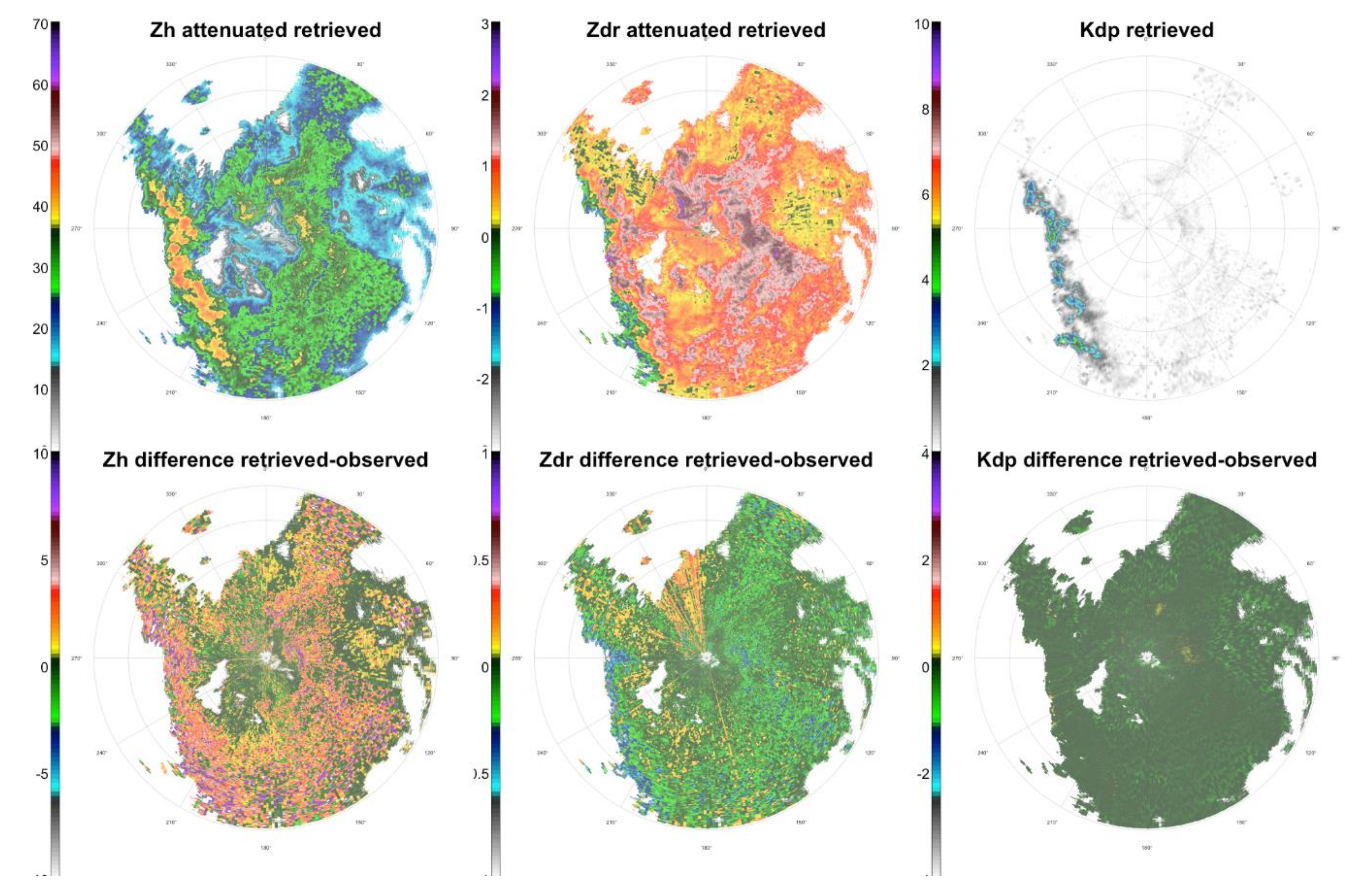
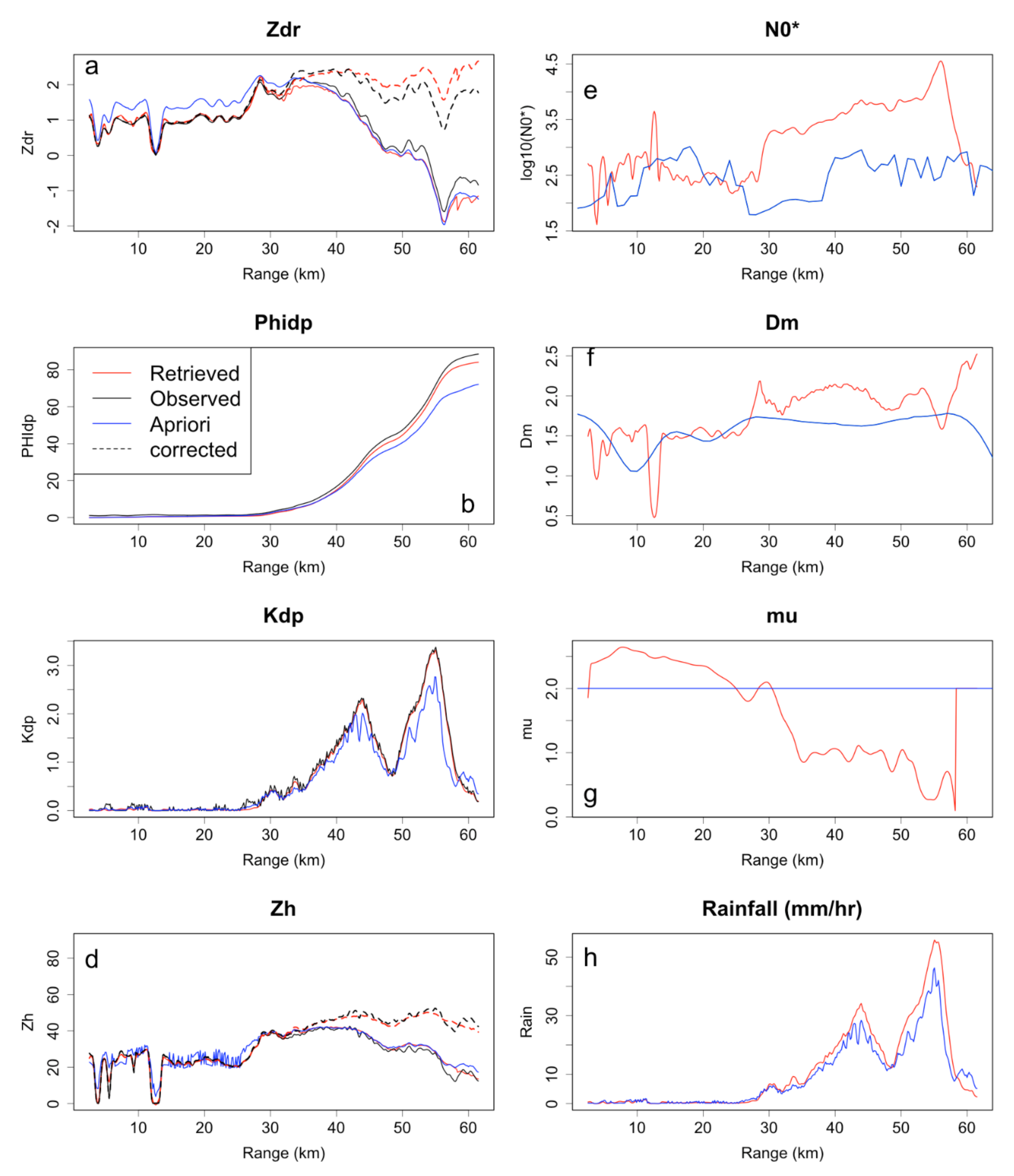
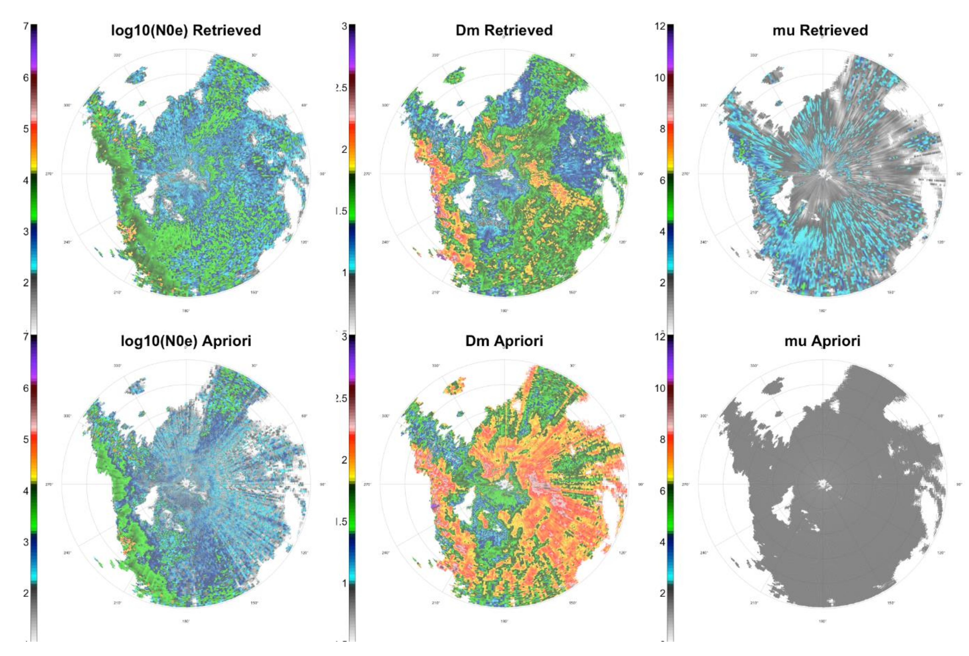
5.1. Retrieved DSD and Gain from an a Priori Solution

Figure 1 illustrates the retrieval along a given radial, extracted from the 28 July 2006 case study (Azimuth 251°; 7h58 UTC; 2.8° elevation PPI). The observed system is typical of African squall lines and $K_{DP}$ shows two peaks of convective rainfall at 42 km and 53 km range, and stratiform rainfall at 30–40 km, while the system is moving away from the radar (Westwards). The left column shows four radar variables along the radial: the observed (thus attenuated) $Z_H$, the attenuated $Z_{DR}$, the differential phase shift ${\Phi }_{DP}$ and the specific differential phase shift $K_{DP}$. On each plot, the observed variables (in black) are displayed together with the radar variables simulated (attenuation included) from a priori DSD (blue) and from the inverse model framework (red). On the right column, the retrieved DSD parameters $N_{0 }^{*},D_{m }, \mu$ (red) are compared with the a priori solution (blue).

The radar variables simulated by the retrieval algorithm are globally closer to the observations than the radar variables only simulated with a priori DSD parameters, thus illustrating that the retrieval algorithm improves a priori estimation by finding a solution more consistent with the observations at the scale of the entire radar radial. The difference between the retrieved solution and the observation is lower for $K_{DP}$ which is due to the low relative uncertainty prescribed on this observation (Section 4.3). In this example, the attenuation is high due to the intense rainfall seen by the X-band radar. It can be noticed that the constraint imposed on ${\Phi }_{DP}$ by Equation (16) is efficient and ensures a low bias in the integrated $K_{DP}$, allowing a good estimation of the attenuation. Concerning $Z_H,$ the observed and retrieved values are very close all along the radial. $Z_{DR}$ show a possible over correction at the end of the radial, probably caused by the use of a fixed oblateness law.

On the right column in Figure 1, the retrieved parameters [$N_0^{*}, D_m$] show peaks at the convective rainfall range (~54 km). The peak of $D_m$ at the end of the radial may be an artifact related to the high peak of $Z_{DR}$: at the end of the radial, the radar signal became closer to the noise level, and the variables were less reliable (also confirmed by low values of the cross-correlation coefficient ${\rho }_{HV}$—not shown).

Figure 2 illustrates the maps of retrieved DSD parameters, and Figure 3 shows the consistency between the observed radar variables and those simulated from the forward model using the retrieved DSDs. The presented PPI is at 2.8° elevation for the 12 September 2006 event at 19:08 UTC. As for Figure 1, the case is typical of an African squall line, with a marked line of convective cells on the West front followed by stratiform rain. The retrieved fields of $N_0^{*}, D_m, \mu$ (Figure 2 top) and from a priori solution based on [8] (Figure 2 bottom) exhibit some differences. The retrieval algorithm leads to a better spatial consistency of the DSD field. The radial stripes that appear on the field $N_0^{*}$ for a priori (bottom left in Figure 2) have disappeared after applying the retrieval algorithm (top left in Figure 2). The stripes in a priori solution are quite typical of radial-to-radial inconsistency in ${\varphi }_{DP}$ which have a strong effect on the DSD retrieval when the attenuation correction based on this variable is applied prior to -and independently of- the retrieval (the 2-step problem already noticed by [38]. The improved radial to radial consistency obtained with the retrieval algorithm is noteworthy as this is not imposed by the algorithm (only a spatial correlation of 3km inside the radial is imposed by the covariance matrix)—it is an indirect benefit of the retrieval method, which absorbs better the observation uncertainty. The previously observed jump [43] between the relatively high value of $N_0^{*}$ in the convective cells and lower values in the stratiform parts is well reproduced in the field. The stratiform and convective regions are clearly differentiable. Comparing a priori field of $N_0^{*}$ and the retrieved, we observe clusters of high $N_0^{*}$ values in the convective region of the retrieved field (yellow dots) associated with convective cells, which are less highlighted in a priori field. A global overestimation of $D_m$ in a priori is corrected by the algorithm—this will be further confirmed by the results in Figure 4.

The retrieved values for μ are globally higher than a priori value (constant $\mu =2$) and especially in the convective part. This is consistent with what was observed statistically with the disdrometer by [43]. The radar variables have a relatively low sensitivity to $\mu$ (except for $Z_{DR}$) and $\mu$ is therefore less constrained by the observations than the two other DSD parameters. The retrieved values of $\mu$ appear weakly correlated with the retrieved values of $D_m$ without imposing such cofluctuation in the retrieval algorithm. According to prior studies using disdrometer data [12,20] $D_m$ and $\mu$ are anticorrelated, which is in contradiction with our results. On the other hand, [47] did not find any evidence of $D_m$-$\mu$ relation on the present dataset. Probably $\mu$ is absorbing the noise in the retrieval procedure.

Figure 3 shows the radar variables simulated with the forward model and the retrieved DSDs and the absolute errors with respect to the observed fields (residuals). For $K_{DP}$ the residuals are non-biased (thanks to the strong constraint on ${\varphi }_{DP}$ at the end of each radial). $Z_{DR}$ shows little or no bias in the fields indistinctly of the type of rainfall. All the errors in the model are absorbed by $Z_H$ in the convective part, where the attenuation is high. As seen in the residual map of $Z_H$ (Figure 3 bottom left), there is a positive bias in the retrieved $Z_H$ in the convective region. The same bias can be observed in Figure 1d in the retrieved $Z_H$ at 54 km.

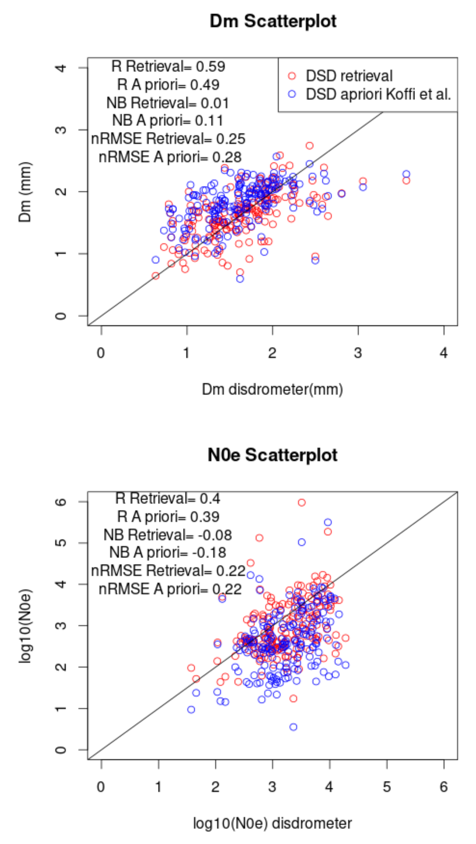
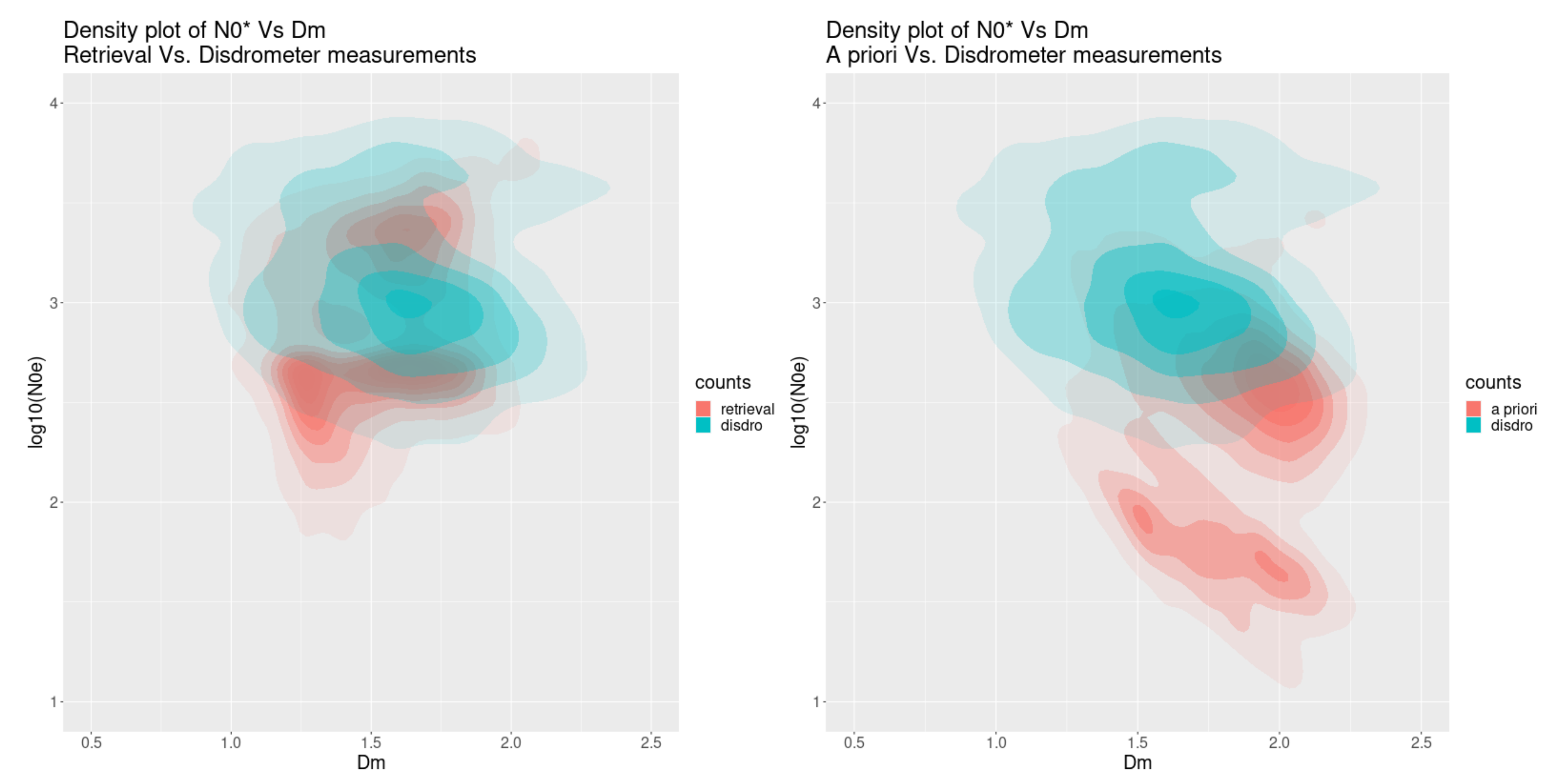
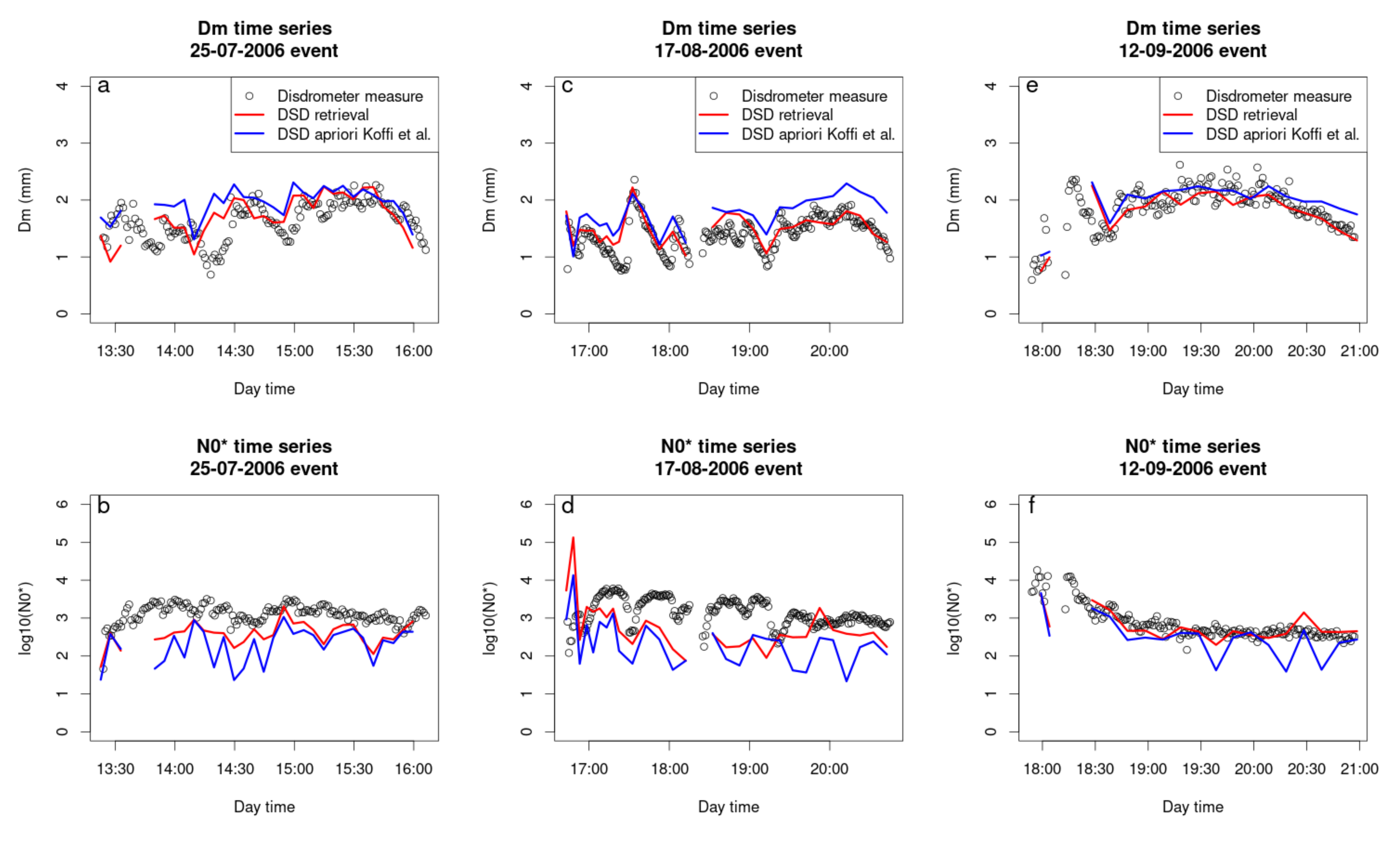
5.2. Comparison of Disdrometer and Radar Derived DSD

In this section, we compare the collocated radar retrieved and disdrometer DSDs. The comparisons are performed for all the organized convective systems observed on site in 2006, as summarized in Table 1. The comparisons are for the disdrometer situated in Copargo, 18 km from the radar. At the disdrometer range, the volume scan of the radar is between 0.7 and 1.2 km height considering a $\pm 0.7°$ radar aperture angle. Considering the typical fall speed of drops, we could expect a few minutes shift between the radar aloft and disdrometer observation at the ground.

Figure 4 shows the time series of DSD parameters retrieved by the radar (a priori and final result) and observed by the disdrometer for three cases that illustrate the variety of obtained results. The retrieved DSD (red) exhibits a good dynamic through the three events when compared with the disdrometer (black circles), and the consistency is better than a priori solution (blue). The improvement between a priori and retrieved solutions is more marked for $N_0^{*}$; the retrieved is much smoother than the a priori value and closer to the ground reference. Nevertheless, a bias on $N_0^{*}$ appears for some events (the highest on 17 August 2006) and is only partially corrected by the retrieval algorithm. A calibration problem on the reflectivities could be the cause of this retrieved bias on $N_0^{*}$—at the moment the calibration constant is not parameterized in the inverse model but could be included in a future extension of the model.

Figure 5 displays the scatter plot of retrieved DSD parameters versus collocated disdrometer measurements for all events reported in Table 1. The improvement of the inverse method compared to the a priori two-step method is visible. The global statistics are improved in terms of correlation and bias, with a slight reduction in nRMSE for Dm). Note that the retrieval skill is almost unchanged when a calibration error of + or—2dBZ is applied to the reflectivities (not shown, see

Table A1. Sensitivity to calibration. Averaged normalized bias in % for the three retrieved parameters (and rainfall) in the a a priori and retrieved solution in convective and stratiform radar gates. Four different perturbation are tested $\pm 2 \mathrm{dB}$ in $Z_h$ and $\pm 0.2 \mathrm{dB}$ in $Z_{DR}$.

			$+2 \mathbf{dB} {\mathit{Z}}_{\mathit{H}}$	$-2 \mathbf{dB} {\mathit{Z}}_{\mathit{H}}$	$+0.2 \mathbf{dB} {\mathit{Z}}_{\mathit{D}\mathit{R}}$	$-0.2 \mathbf{dB} {\mathit{Z}}_{\mathit{D}\mathit{R}}$
Conv	$\mathsf{\Delta }{N}_0^{*}$	Apr.	53.9	17.5	−0.5	33.4
		Retr.	−15.2	26.9	−10.3	29.4
	$\mathsf{\Delta }{D}_m$	Apr.	2.5	−1.8	2.8	−2.3
		Retr.	2.9	−1.8	2.2	−2.3
	$\mathsf{\Delta }\mu$	Apr.	-	-	-	-
		Retr.	112.8	52.4	108.3	86.8
	$\mathsf{\Delta }Rain$	Apr.	16.8	−14.2	−2.8	3.1
		Retr.	−5.7	4.8	−3.1	3.6
Strat	$\mathsf{\Delta }{N}_0^{*}$	Apr.	20.9	−14.3	−27.1	125.7
		Retr.	−21.7	27.2	−13.4	108.4
	$\mathsf{\Delta }{D}_m$	Apr.	0.3	0.0	6.2	−5.8
		Retr.	7.0	−4.2	3.0	−3.4
	$\mathsf{\Delta }\mu$	Apr.	-	-	-	-
		Retr.	17.1	−4.8	−14.3	17.3
	$\mathsf{\Delta }Rain$	Apr.	19.4	−16.4	−6.2	7.4
		Retr.	2.0	0.3	−4.6	15.8

).

Figure 5 indicates an improvement in DSD retrieval. However, some differences remain between the disdrometer and radar retrieved DSDs. The distribution of median diameter D_m is narrower on radar than on the disdrometer dataset. Some of these differences are unavoidable given the different nature of the two datasets. The radar samples a larger volume of the atmosphere and higher above ground than the disdrometer. We can also notice that the disdrometer has points for Dm > 2.7 mm that the retrieval has not. This can be caused by excessive filtering of the polarimetric variables or a wrong representation of the oblateness low.

Figure 6 illustrates the improvement in DSD retrieval compared to a priori solution over the entire disdrometer record. The figure shows the density plot of observed [$N_0^{*}, D_m$] pairs, superimposing the disdrometer (blue) and radar (red) derived datasets. We used radar retrieval of the 12 September 2006 event (7 PPI from 17:59 UTC to 18:48). The disdrometer statistics include all the events sampled for the 2006 and 2007 rainy seasons. The overall agreement is stronger for the inverse method (left plot) than for a priori solution based on [8]. In particular, the range of retrieved $N_0^{*}$ is better matched with the disdrometer for the inverse method, while a priori solution generates lower values. We can also observe that the retrieval reproduces the convective precipitation distribution of [$N_0^{*}, D_m$], which is the blue hook around $D_m>1.75$ and $log10(N_0^{*})>3.5$. A priori solution seems also to reproduce a shifted hook, around $D_m ~ 2$ and $log10(N_0^{*})~3.25$.

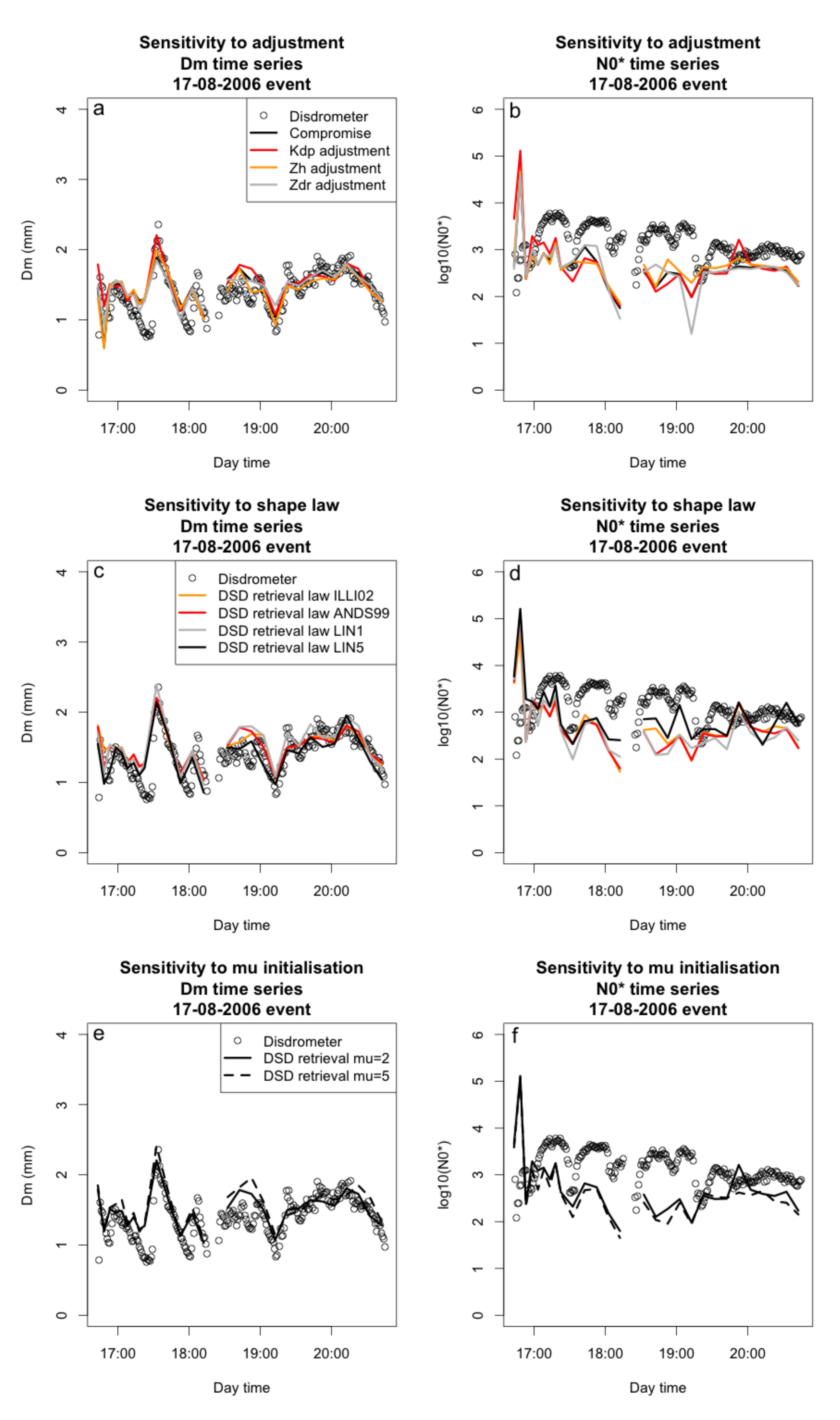
5.3. Sensitivity to Calibration and Model Parameters

The sensitivity test results are presented in detail in the Appendix B.

6. Discussion

The objectives of the implemented methodology are reminded: the proposed algorithm starts with a benchmark method (a priori solution), based on simple parametric formulae (Equations (5) and (6), and Section 4.3); this a priori solution is then improved using the inverse theory framework (Section 4.1) in order to ‘inject in the solution’ what is known about the physics, i.e., the interaction between the drops and the radar wave (Section 3). The physics, described in the forward model (Section 3), relates the properties of the drop size distributions along the radar beam to the polarimetric radar variables and accounts explicitly for the attenuation. In the current implementation, the result of the retrieval once applied to the three independent measured radar variables ($Z_{h }^{att},{ Z}_{dr }^{att},{ K}_{dp }$) of a PPI, is a field of three DSD variables ($N_{0 }^{*},D_{m }, \mu$) as described in Section 3 and Section 4.

One expected benefit from the inverse retrieval is an improvement compared to the benchmark by providing a solution that better accounts for the consistency among the measured variables along each beam. The objective is to achieve the best coherence between the various sources of information available (observed data; a priori solution; forward model) while accounting for the degree of confidence in each source (measurement noise; trust in the forward model; trust in the a priori etc.) as described in Section 4.1.

Figure 2, which compared a priori DSD field with the retrieved one, is a visual illustration of the benefit of the inverse framework. In the benchmark method, some radials were inconsistent with their neighbors, showing a ray-like pattern of high $N_0^{*}$, which does not fit with rain microphysics. The inverse method brought spatial consistency.

Figure 4, Figure 5 and Figure 6, which compared the radar-derived values of $N_0^{*}$ and $D_m$ with those observed by disdrometers, confirm that the retrieval is closer to the observations than a priori is. Compared to a priori, the retrieved solution is characterized by globally lower values of the median diameter $D_m$ and, to a lesser extent, higher values of $N_0^{*}$. This shift is clear on the maps (Figure 2). Figure 4, Figure 5 and Figure 6 confirm that these characteristics are closer to the observations.

The retrieval has relative skill compared to a priori. Can it, however, be considered satisfactory in absolute terms? Figure 4, Figure 5 and Figure 6 show that the match between the retrieved and observed DSDs is indeed not perfect. In the first two events of Figure 4, the retrieved $D_m$ are close to the observations, but a negative bias remains in $N_0^{*}$, even though less marked than for the a priori. The statistics in Figure 5 show that the overall bias, all events considered, is very low. However, some spread is visible, and the nRMSE is about 25% for $D_m$ and 22% for $N_0^{*}$. Comparing results with other studies is difficult as the scores used, the sample size, and the experimental contexts are different. Our nRMSE are of the same order of magnitude—or slightly higher—such as those reported by [25] or [22] The retrieved biases are similar or lower than those reported in the literature [24,26]. None of the other studies that reported direct comparisons between radar and DSDs used an attenuated frequency, and no other experiment was in Africa, dealing with intense convection. The few studies which evaluated DSD retrieval for attenuating frequencies were based on simulations [38] and cannot be compared with actual observations.

The non-negligible errors reported in all studies that compared observed DSDs with radar retrieval have been discussed by various authors [23,64]. An important source of error is the difference in spatio-temporal sampling between a disdrometer at ground level and the resolution volume of a radar. A typical change-of-support problem is expected to introduce error spread (e.g., [48]). The limited sampling volume of a disdrometer can lead to errors in the estimation of the DSD. According to [65], who used a collocated set of 14 disdrometers in Spain, at least 5 disdrometers or a surface of 370 cm² are necessary to provide a robust estimation of the DSD parameters. The problem is expected to be more acute in Africa, where the intense convective rainfall exhibits high spatiotemporal variability and where the presence of big drops may be a challenge for disdrometers.

7. Conclusions

An inverse method to retrieve fields of DSD parameters from radar polarimetric observations at attenuated frequency is presented and tested on X-band data in Africa. Three parameters of a gamma DSD (the volume-weighted mean diameter $D_m$, the scaling parameter of concentration $N_0^{*}$ and a shape parameter, $\mu$) are retrieved at each range gate along a radial. The estimation of the DSD parameters using empirical power laws suited to the local climatology is used as prior information to an inverse algorithm which then finds the solution which best matches the entire radar radial observations. In line with the approach developed by [38], this framework ensures a global consistency between the retrieved DSD and all radar variables. It reduces the errors brought by the uncertainty in the attenuation correction procedure. The iterative algorithm makes use of a strong constraint –like the differential phase shift at the last gate—to ensure robustness.

The forward model needed by the retrieval algorithm relates the observed radar variables to the DSD along the radial. This model is based on explicit calculations of radar variables (reflectivities in horizontal and vertical polarization; specific differential phase shift; specific attenuation coefficient for each polarization) as a function of drop sizes and shapes. T-matrix calculations for drops considered as oblate spheroids were used for this purpose. By convoluting the T-matrix output and the DSD, the radar variables were pre-calculated for gamma DSD over a range of values of the three parameters of interest $D_m$, $N_0^{*}$ and $\mu$. These calculations were made for several assumptions concerning the aspect ratio of drops and the sensitivity to the prescribed temperature also analyzed (and found to be small). In addition to (i) the observed radar variables and (ii) the radial profile of the 3 DSD parameters to be retrieved, many other parameters and a priori information need to be prescribed to the inverse model

The results of the inversion were evaluated through direct comparisons with disdrometer data and also by analyzing the global consistency of the retrieved DSD maps compared to the ‘2 step’ empirical method from [8]. Fifteen rainfall events, for a total of 244 PPI, were used for direct comparison between the disdrometer and the radar DSD retrieved at the closest pixel. The correlation between the time series, of $D_m$ and for $N_0^{*}$ is increased from r = 0.49 for a priori estimate to r = 0.58 for the final solution, and the normalized bias is significantly reduced for both $N_0^{*}$ and $D_m$. These numbers are similar to the scores obtained when radar retrieved DSD is compared with disdrometer data in other studies [23] at non-attenuating frequencies. This is quite remarkable given the intense attenuation encountered in the study region in West Africa.

Compared to empirical methods, the proposed retrieval algorithm, by providing an overall retrieval of the range profile of DSD, leads to a solution that is more consistent with all observed radar variables and shows a better spatial consistency. This is apparent on the retrieved DSD maps based on any given PPI; the spurious radials that tend to appear with the 2 steps method because of errors brought by the attenuation correction disappear with the retrieval method.

These results appear promising, but a more comprehensive assessment of the proposed method is required. For that purpose, various datasets representative of different climatological contexts are needed. In addition, it would be interesting to compare the present method with the method proposed by [38] in order to assess their respective advantages and drawbacks and to explicitly take into account the differential phase shift in the formulation of the inverse algorithm. If these methods were to be used with operational radars and in real-time, the optimization of the processing time compared to retrieval accuracy should be analyzed. Some improvements and new implementations could be added to the inverse model. In the current version, the calibration of reflectivities is assumed to be correct, but a calibration (slowly varying) constant could be added to the model and retrieved as a parameter. In future versions of the algorithm, we will consider including the parameter $\beta$ (slope of the axis ratio law as in [18] to adjust the axis ratio law for different events.

References

1. Atlas, D.; Ulbrich, C.W.; Marks, F.D.; Amitai, E.; Williams, C.R. Systematic Variation of Drop Size and Radar-Rainfall Relations. J. Geophys. Res. Atmos. 1999, 104, 6155–6169. [Google Scholar] [CrossRef]
2. Lee, G.W.; Zawadzki, I. Variability of Drop Size Distributions: Time-Scale Dependence of the Variability and Its Effects on Rain Estimation. J. Appl. Meteorol. 2005, 44, 241–255. [Google Scholar] [CrossRef]
3. Lee, G.W.; Zawadzki, I.; Szyrmer, W.; Sempere-Torres, D.; Uijlenhoet, R. A General Approach to Double-Moment Normalization of Drop Size Distributions. J. Appl. Meteorol. 2004, 43, 264–281. [Google Scholar] [CrossRef]
4. Steiner, M.; Smith, J.A.; Uijlenhoet, R. A Microphysical Interpretation of Radar Reflectivity–Rain Rate Relationships. J. Atmos. Sci. 2004, 61, 1114–1131. [Google Scholar] [CrossRef]
5. Uijlenhoet, R.; Steiner, M.; Smith, J.A. Variability of Raindrop Size Distributions in a Squall Line and Implications for Radar Rainfall Estimation. J. Hydrometeorol. 2003, 4, 43–61. [Google Scholar] [CrossRef]
6. Cao, Q.; Zhang, G.; Brandes, E.; Schuur, T.; Ryzhkov, A.; Ikeda, K. Analysis of Video Disdrometer and Polarimetric Radar Data to Characterize Rain Microphysics in Oklahoma. J. Appl. Meteorol. Climatol. 2008, 47, 2238–2255. [Google Scholar] [CrossRef] [Green Version]
7. Vivekanandan, J.; Zhang, G.; Brandes, E. Polarimetric Radar Estimators Based on a Constrained Gamma Drop Size Distribution Model. J. Appl. Meteorol. 2004, 43, 217–230. [Google Scholar] [CrossRef]
8. Koffi, A.K.; Gosset, M.; Zahiri, E.-P.; Ochou, A.D.; Kacou, M.; Cazenave, F.; Assamoi, P. Evaluation of X-Band Polarimetric Radar Estimation of Rainfall and Rain Drop Size Distribution Parameters in West Africa. Atmos. Res. 2014, 143, 438–461. [Google Scholar] [CrossRef]
9. Bringi, V.N.; Huang, G.-J.; Chandrasekar, V.; Gorgucci, E. A Methodology for Estimating the Parameters of a Gamma Raindrop Size Distribution Model from Polarimetric Radar Data: Application to a Squall-Line Event from the TRMM/Brazil Campaign. J. Atmos. Ocean. Technol. 2002, 19, 633–645. [Google Scholar] [CrossRef]
10. Janapati, J.; Seela, B.K.; Lin, P.-L.; Wang, P.K.; Kumar, U. An Assessment of Tropical Cyclones Rainfall Erosivity for Taiwan. Sci. Rep. 2019, 9, 15862. [Google Scholar] [CrossRef] [Green Version]
11. Protat, A.; Klepp, C.; Louf, V.; Petersen, W.A.; Alexander, S.P.; Barros, A.; Leinonen, J.; Mace, G.G. The Latitudinal Variability of Oceanic Rainfall Properties and Its Implication for Satellite Retrievals: 2. The Relationships Between Radar Observables and Drop Size Distribution Parameters. JGR Atmos. 2019, 124, 13312–13324. [Google Scholar] [CrossRef]
12. Protat, A.; Klepp, C.; Louf, V.; Petersen, W.A.; Alexander, S.P.; Barros, A.; Leinonen, J.; Mace, G.G. The Latitudinal Variability of Oceanic Rainfall Properties and Its Implication for Satellite Retrievals: 1. Drop Size Distribution Properties. JGR Atmos. 2019, 124, 13291–13311. [Google Scholar] [CrossRef]
13. Torres, D.S.; Porrà, J.M.; Creutin, J.-D. A General Formulation for Raindrop Size Distribution. J. Appl. Meteorol. 1994, 33, 1494–1502. [Google Scholar] [CrossRef]
14. Testud, J.; Oury, S.; Black, R.A.; Amayenc, P.; Dou, X. The Concept of “Normalized” Distribution to Describe Raindrop Spectra: A Tool for Cloud Physics and Cloud Remote Sensing. J. Appl. Meteorol. 2001, 40, 1118–1140. [Google Scholar] [CrossRef]
15. Lee, C.K.; Lee, G.W.; Zawadzki, I.; Kim, K.-E. A Preliminary Analysis of Spatial Variability of Raindrop Size Distributions during Stratiform Rain Events. J. Appl. Meteorol. Climatol. 2009, 48, 270–283. [Google Scholar] [CrossRef]
16. Gorgucci, E.; Scarchilli, G.; Chandrasekar, V.; Bringi, V.N. Rainfall Estimation from Polarimetric Radar Measurements: Composite Algorithms Immune to Variability in Raindrop Shape–Size Relation. J. Atmos. Ocean. Technol. 2001, 18, 1773–1786. [Google Scholar] [CrossRef]
17. Gorgucci, E.; Chandrasekar, V.; Bringi, V.N.; Scarchilli, G. Estimation of Raindrop Size Distribution Parameters from Polarimetric Radar Measurements. J. Atmos. Sci. 2002, 59, 2373–2384. [Google Scholar] [CrossRef]
18. Gorgucci, E.; Chandrasekar, V.; Baldini, L. Can a Unique Model Describe the Raindrop Shape–Size Relation? A Clue from Polarimetric Radar Measurements. J. Atmos. Ocean. Technol. 2009, 26, 1829–1842. [Google Scholar] [CrossRef]
19. Zhang, G.; Vivekanandan, J.; Brandes, E. A Method For Estimating Rain Rate And Drop Size Distribution From Polarimetric Radar Measurements. IEEE Trans. Geosci. Remote Sens. 2021, 4, 830–841. [Google Scholar]
20. Brandes, E.A.; Zhang, G.; Vivekanandan, J. Drop Size Distribution Retrieval with Polarimetric Radar: Model and Application. J. Appl. Meteorol. 2004, 43, 461–475. [Google Scholar] [CrossRef]
21. Kim, D.-S.; Maki, M.; Lee, D.-I. Retrieval of Three-Dimensional Raindrop Size Distribution Using X-Band Polarimetric Radar Data. J. Atmos. Ocean. Technol. 2010, 27, 1265–1285. [Google Scholar] [CrossRef]
22. Anagnostou, M.N.; Anagnostou, E.N.; Vulpiani, G.; Montopoli, M.; Marzano, F.S.; Vivekanandan, J. Evaluation of X-Band Polarimetric-Radar Estimates of Drop-Size Distributions From Coincident S-Band Polarimetric Estimates and Measured Raindrop Spectra. IEEE Trans. Geosci. Remote Sens. 2008, 46, 3067–3075. [Google Scholar] [CrossRef]
23. Raupach, T.H.; Berne, A. Retrieval of the Raindrop Size Distribution from Polarimetric Radar Data Using Double-Moment Normalisation. Atmos. Meas. Tech. 2017, 10, 2573–2594. [Google Scholar] [CrossRef] [Green Version]
24. Islam, T.; Rico-Ramirez, M.A.; Han, D. Tree-Based Genetic Programming Approach to Infer Microphysical Parameters of the DSDs from the Polarization Diversity Measurements. Comput. Geosci. 2012, 48, 20–30. [Google Scholar] [CrossRef]
25. Cao, Q.; Zhang, G.; Brandes, E.A.; Schuur, T.J. Polarimetric Radar Rain Estimation through Retrieval of Drop Size Distribution Using a Bayesian Approach. J. Appl. Meteorol. Climatol. 2010, 49, 973–990. [Google Scholar] [CrossRef]
26. Wen, G.; Chen, H.; Zhang, G.; Sun, J. An Inverse Model for Raindrop Size Distribution Retrieval with Polarimetric Variables. Remote Sens. 2018, 10, 1179. [Google Scholar] [CrossRef] [Green Version]
27. Kim, D.-S.; Maki, M.; Lee, D.-I. Correction of X-Band Radar Reflectivity and Differential Reflectivity for Rain Attenuation Using Differential Phase. Atmos. Res. 2008, 90, 1–9. [Google Scholar] [CrossRef]
28. Park, S.G.; Maki, M.; Iwanami, K.; Bringi, V.N.; Chandrasekar, V. Correction of Radar Reflectivity and Differential Reflectivity for Rain Attenuation at X Band. Part II: Evaluation and Application. J. Atmos. Ocean. Technol. 2005, 22, 1633–1655. [Google Scholar] [CrossRef]
29. Shi, Z.; Chen, H.; Chandrasekar, V.; He, J. Deployment and Performance of an X-Band Dual-Polarization Radar during the Southern China Monsoon Rainfall Experiment. Atmosphere 2017, 9, 4. [Google Scholar] [CrossRef] [Green Version]
30. Bringi, V.N.; Keenan, T.D.; Chandrasekar, V. Correcting C-Band Radar Reflectivity and Differential Reflectivity Data for Rain Attenuation: A Self-Consistent Method with Constraints. IEEE Trans. Geosci. Remote Sens. 2001, 39, 1906–1915. [Google Scholar] [CrossRef]
31. Testud, J.; Le Bouar, E.; Obligis, E.; Ali-Mehenni, M. The Rain Profiling Algorithm Applied to Polarimetric Weather Radar. J. Atmos. Ocean. Technol. 2000, 17, 332–356. [Google Scholar] [CrossRef]
32. Matrosov, S.Y.; Clark, K.A.; Martner, B.E.; Tokay, A. X-Band Polarimetric Radar Measurements of Rainfall. J. Appl. Meteorol. 2002, 41, 941–952. [Google Scholar] [CrossRef]
33. Kalogiros, J.; Anagnostou, M.N.; Anagnostou, E.N.; Montopoli, M.; Picciotti, E.; Marzano, F.S. Evaluation of a New Polarimetric Algorithm for Rain-Path Attenuation Correction of X-Band Radar Observations Against Disdrometer. IEEE Trans. Geosci. Remote Sens. 2014, 52, 1369–1380. [Google Scholar] [CrossRef]
34. Gou, Y.; Chen, H.; Zheng, J. An Improved Self-Consistent Approach to Attenuation Correction for C-Band Polarimetric Radar Measurements and Its Impact on Quantitative Precipitation Estimation. Atmos. Res. 2019, 226, 32–48. [Google Scholar] [CrossRef]
35. Gosset, M.; Zahiri, E.-P.; Moumouni, S. Rain Drop Size Distribution Variability and Impact on X-Band Polarimetric Radar Retrieval: Results from the AMMA Campaign in Benin. Q. J. R. Meteorol. Soc. 2010, 136, 243–256. [Google Scholar] [CrossRef]
36. Matrosov, S.Y.; Kingsmill, D.E.; Martner, B.E.; Ralph, F.M. The Utility of X-Band Polarimetric Radar for Quantitative Estimates of Rainfall Parameters. J. Hydrometeorol. 2005, 6, 248–262. [Google Scholar] [CrossRef] [Green Version]
37. Chang, W.-Y.; Vivekanandan, J.; Chen Wang, T.-C. Estimation of X-Band Polarimetric Radar Attenuation and Measurement Uncertainty Using a Variational Method. J. Appl. Meteorol. Climatol. 2014, 53, 1099–1119. [Google Scholar] [CrossRef]
38. Yoshikawa, E.; Chandrasekar, V.; Ushio, T. Raindrop Size Distribution (DSD) Retrieval for X-Band Dual-Polarization Radar. J. Atmos. Ocean. Technol. 2014, 31, 387–403. [Google Scholar] [CrossRef]
39. Tarantola, A. Inverse Problem Theory and Methods for Model Parameter Estimation; Society for Industrial and Applied Mathematics: Philadelphia, PA, USA, 2005; Volume 89, ISBN 0-89871-792-2. [Google Scholar]
40. Menke, W. Geophysical Data Analysis: Discrete Inverse Theory, 4th ed.; Elsevier: Amsterdam, The Netherlands; Academic Press: Cambridge, MA, USA, 2018; ISBN 978-0-12-813555-6. [Google Scholar]
41. Lebel, T.; Parker, D.J.; Flamant, C.; Bourlès, B.; Marticorena, B.; Mougin, E.; Peugeot, C.; Diedhiou, A.; Haywood, J.M.; Ngamini, J.B.; et al. The AMMA Field Campaigns: Multiscale and Multidisciplinary Observations in the West African Region. Q. J. R. Meteorol. Soc. 2010, 136, 8–33. [Google Scholar] [CrossRef]
42. Depraetere, C.; Gosset, M.; Ploix, S.; Laurent, H. The Organization and Kinematics of Tropical Rainfall Systems Ground Tracked at Mesoscale with Gages: First Results from the Campaigns 1999–2006 on the Upper Ouémé Valley (Benin). J. Hydrol. 2009, 375, 143–160. [Google Scholar] [CrossRef]
43. Moumouni, S.; Gosset, M.; Houngninou, E. Main Features of Rain Drop Size Distributions Observed in Benin, West Africa, with Optical Disdrometers. Geophys. Res. Lett. 2008, 35. [Google Scholar] [CrossRef]
44. Cazenave, F.; Gosset, M.; Kacou, M.; Alcoba, M.; Fontaine, E.; Duroure, C.; Dolan, B. Characterization of Hydrometeors in Sahelian Convective Systems with an X-Band Radar and Comparison with in Situ Measurements. Part I: Sensitivity of Polarimetric Radar Particle Identification Retrieval and Case Study Evaluation. J. Appl. Meteorol. Climatol. 2016, 55, 231–249. [Google Scholar] [CrossRef]
45. Hubbert, J.; Bringi, V.N. An Iterative Filtering Technique for the Analysis of Copolar Differential Phase and Dual-Frequency Radar Measurements. J. Atmos. Ocean. Technol. 1995, 12, 643–648. [Google Scholar] [CrossRef]
46. Delahaye, J.-Y.; Barthès, L.; Golé, P.; Lavergnat, J.; Vinson, J.P. A Dual-Beam Spectropluviometer Concept. J. Hydrol. 2006, 328, 110–120. [Google Scholar] [CrossRef]
47. Moumouni, S. Analyse Des Distributions Granulométriques Des Pluies Au Bénin: Caractéristiques Globales, Variabilité et Application à La Mesure Radar. Ph.D. Thesis, Ecole Normale Supérieure Natitingou, Université de Parakou, Parakou, Bénin, 2009. [Google Scholar]
48. Tokay, A.; Short, D.A. Evidence from Tropical Raindrop Spectra of the Origin of Rain from Stratiform versus Convective Clouds. J. Appl. Meteorol. 1996, 35, 355–371. [Google Scholar] [CrossRef]
49. Alcoba, M.; Gosset, M.; Kacou, M.; Cazenave, F.; Fontaine, E. Characterization of Hydrometeors in Sahelian Convective Systems with an X-Band Radar and Comparison with in Situ Measurements. Part II: A Simple Brightband Method to Infer the Density of Icy Hydrometeors. J. Appl. Meteorol. Climatol. 2016, 55, 251–263. [Google Scholar] [CrossRef]
50. Trömel, S.; Kumjian, M.R.; Ryzhkov, A.V.; Simmer, C.; Diederich, M. Backscatter Differential Phase—Estimation and Variability. J. Appl. Meteorol. Climatol. 2013, 52, 2529–2548. [Google Scholar] [CrossRef] [Green Version]
51. Giangrande, S.E.; McGraw, R.; Lei, L. An Application of Linear Programming to Polarimetric Radar Differential Phase Processing. J. Atmos. Ocean. Technol. 2013, 30, 1716–1729. [Google Scholar] [CrossRef]
52. Schneebeli, M.; Berne, A. An Extended Kalman Filter Framework for Polarimetric X-Band Weather Radar Data Processing. J. Atmos. Ocean. Technol. 2012, 29, 711–730. [Google Scholar] [CrossRef]
53. Otto, T.; Russchenberg, H.W.J. Estimation of Specific Differential Phase and Differential Backscatter Phase From Polarimetric Weather Radar Measurements of Rain. IEEE Geosci. Remote Sens. Lett. 2011, 8, 988–992. [Google Scholar] [CrossRef]
54. Reinoso-Rondinel, R.; Unal, C.; Russchenberg, H. Adaptive and High-Resolution Estimation of Specific Differential Phase for Polarimetric X-Band Weather Radars. J. Atmos. Ocean. Technol. 2018, 35, 555–573. [Google Scholar] [CrossRef]
55. Bringi, V.N.; Chandrasekar, V. Polarimetric Doppler Weather Radar: Principles and Applications; Cambridge University Press: Cambridge, UK, 2001; ISBN 1-139-42946-9. [Google Scholar]
56. Beard, K.V.; Bringi, V.N.; Thurai, M. A New Understanding of Raindrop Shape. Atmos. Res. 2010, 97, 396–415. [Google Scholar] [CrossRef]
57. Szakáll, M.; Mitra, S.K.; Diehl, K.; Borrmann, S. Shapes and Oscillations of Falling Raindrops—A Review. Atmos. Res. 2010, 97, 416–425. [Google Scholar] [CrossRef]
58. Gorgucci, E.; Baldini, L.; Chandrasekar, V. What Is the Shape of a Raindrop? An Answer from Radar Measurements. J. Atmos. Sci. 2006, 63, 3033–3044. [Google Scholar] [CrossRef]
59. Andsager, K.; Beard, K.V.; Laird, N.F. Laboratory Measurements of Axis Ratios for Large Raindrops. J. Atmos. Sci. 1999, 56, 2673–2683. [Google Scholar] [CrossRef]
60. Mishchenko, M.I.; Travis, L.D.; Mackowski, D.W. T-Matrix Computations of Light Scattering by Nonspherical Particles: A Review. J. Quant. Spectrosc. Radiat. Transf. 1996, 55, 535–575. [Google Scholar] [CrossRef]
61. Waterman, P.C. Matrix Formulation of Electromagnetic Scattering. Proc. IEEE 1965, 53, 805–812. [Google Scholar] [CrossRef]
62. Waterman, P.C. Symmetry, Unitarity, and Geometry in Electromagnetic Scattering. Phys. Rev. D 1971, 3, 825–839. [Google Scholar] [CrossRef]
63. Tarantola, A.; Valette, B. Generalized Nonlinear Inverse Problems Solved Using the Least Squares Criterion. Rev. Geophys. 1982, 20, 219. [Google Scholar] [CrossRef]
64. Adirosi, E.; Baldini, L.; Tokay, A. Rainfall and DSD Parameters Comparison between Micro Rain Radar, Two-Dimensional Video and Parsivel2 Disdrometers, and S-Band Dual-Polarization Radar. J. Atmos. Ocean. Technol. 2020, 37, 621–640. [Google Scholar] [CrossRef]
65. Tapiador, F.J.; Navarro, A.; Moreno, R.; Jiménez-Alcázar, A.; Marcos, C.; Tokay, A.; Durán, L.; Bodoque, J.M.; Martín, R.; Petersen, W.; et al. On the Optimal Measuring Area for Pointwise Rainfall Estimation: A Dedicated Experiment with 14 Laser Disdrometers. J. Hydrometeorol. 2017, 18, 753–760. [Google Scholar] [CrossRef] [Green Version]
Figure 1. Example of the observed, a priori and retrieved polar variables and DSD parameters for a given radial (251° azimuth of 28 July 2006 07:58 2.8° elevation PPI). (ad): Values of the indicated 4 radar variables as a function of range: the attenuated Z D R , the differential phase shift Φ D P , the specific differential phase shift K D P   and   the   attenuated   Z H . On each plot the observed variables (in black) are displayed together with the radar variables simulated (attenuation included) from a priori DSD (blue) and from the inverse model framework (red). On (ad) the dotted lines are the attenuation corrected reflectivities Z D R , Z H , in red, based on the inverse method and in black, based on the Bringi et al. (2001) method (see text), (fh) the 3 retrieved DSD parameters N 0   * , D m   ,   μ (red) are compared with a priori solution (blue).
Remotesensing 14 01116 g001
Figure 2. Retrieved (top) and a priori (bottom) maps of DSD parameters for the 2.8° PPI for the 12 September 2006 event at 19:08 UTC. As indicated the columns, from left to right are for: l o g 10 ( N 0 * ) D m (mm) and μ .
Remotesensing 14 01116 g002
Figure 3. Retrieved fields of radar observables (simulated from the retrieved DSDs using the forward model) and respective residuals relative to the observations. Same PPI than Figure 2. From left to right attenuated   Z H [ dB ],   attenuated   Z D R [ dB ] and K D P [ deg / km ]. Nota: the color bar range is different for the variables (top) and errors (bottom).
Remotesensing 14 01116 g003
Figure 4. Time series of D m (a,c,e) and l o g 10 [ N 0 * ] (b,d,f) retrieved through the inverse method (red), a priori (blue) and observed (black) by the disdrometer for three events. The parameters from the inversion are retrieved at the radar gate where the disdrometer is located (see text). The event in 4e plot is the same event (12 September 2006) as the DSD fields showed in Figure 2 and Figure 3.
Remotesensing 14 01116 g004
Figure 5. Scatterplot of the radar retrieved (Y axis) DSD parameters against the disdrometer (X axis) for collocated radar gate and time step. Top plot, D m bottom, N 0 * . Both a priori (blue) and the inverse method (red) retrieval are shown. The correlation (R), normalized bias (NB) and normalized root mean square error (nRMSE) compared to the disdrometer for both retrievals are indicated on the plots. Eighteen rainy systems for a total of N = 244 collocated points are displayed.
Remotesensing 14 01116 g005
Figure 6. Contour plot on N 0 * - D m distributions of disdrometer DSD and radar retrieved DSD. Left plot: inverse method; Right plot: a priori DSD. The retrieval is for 12 September 2006 event, 7 PPI from 17:59 UTC to 18:48. The disdrometer data is over 2006 and 2007 seasons. The number of N 0 * - D m pairs in each set are: N i n v = 4 × 10 5 points for the retrieval and N d i s d r o = 7 × 10 3 for the disdrometer.
Remotesensing 14 01116 g006