Article

A Flexible Multi-Temporal and Multi-Modal Framework for Sentinel-1 and Sentinel-2 Analysis Ready Data

1
Department of Electronic and Electrical Engineering, University of Strathclyde, Glasgow G1 1XW, UK
2
Department of Chemical and Process Engineering, University of Strathclyde, Glasgow G1 1XJ, UK
3
Computing Systems Laboratory, National Technical University of Athens, 157 80 Athens, Greece
*
Author to whom correspondence should be addressed.
Remote Sens. 2022, 14(5), 1120; https://doi.org/10.3390/rs14051120
Submission received: 31 January 2022 / Revised: 16 February 2022 / Accepted: 21 February 2022 / Published: 24 February 2022
(This article belongs to the Special Issue Sentinel Analysis Ready Data (Sentinel ARD))

Abstract

:
The rich, complementary data provided by Sentinel-1 and Sentinel-2 satellite constellations host considerable potential to transform Earth observation (EO) applications. However, a substantial amount of effort and infrastructure is still required for the generation of analysis-ready data (ARD) from the low-level products provided by the European Space Agency (ESA). Here, a flexible Python framework able to generate a range of consistent ARD aligned with the ESA-recommended processing pipeline is detailed. Sentinel-1 Synthetic Aperture Radar (SAR) data are radiometrically calibrated, speckle-filtered and terrain-corrected, and Sentinel-2 multi-spectral data resampled in order to harmonise the spatial resolution between the two streams and to allow stacking with multiple scene classification masks. The global coverage and flexibility of the framework allows users to define a specific region of interest (ROI) and time window to create geo-referenced Sentinel-1 and Sentinel-2 images, or a combination of both with closest temporal alignment. The framework can be applied to any location and is user-centric and versatile in generating multi-modal and multi-temporal ARD. Finally, the framework handles automatically the inherent challenges in processing Sentinel data, such as boundary regions with missing values within Sentinel-1 and the filtering of Sentinel-2 scenes based on ROI cloud coverage.

1. Introduction

Earth observation (EO) data are an important foundation in support of achieving global-wide development goals as outlined in the United Nations 2030 Agenda for Sustainable Development [1]. Advances in machine learning (ML) and deep learning (DL) techniques have revolutionised the computer vision, natural language processing (NLP) and time series analysis disciplines; however, their adoption in the Earth observation (EO) domain remains comparatively scarce, primarily owing to the challenges with transforming data from satellite providers into analysis-ready formats. The generation of analysis-ready data (ARD) remains heavily reliant on extensive domain knowledge and expertise in managing geospatial data, which in turn restricts the meaningful analysis of large volumes of data. The European Space Agency (ESA) provides free, open access to low-level products, i.e., Levels 1-2; however, the availability of ARD with global coverage remains a major barrier. The infrastructure requirements to generate ARD products are demanding as satellite data processing is both computationally and memory-intensive. The ready availability of ARD in a format amenable to the development of ML and DL applications would yield unprecedented opportunities to exploit under-utilised satellite data to develop solutions to global challenges such as flood risk mapping [2], water resource management [3], deforestation [4] and glacial lake mapping [5]. Collocated Sentinel-1 and Sentinel-2 data are also used in applications such as land cover mapping [6], crop type classification [7], cloud removal [8], and soil moisture mapping [9].
A number of analysis-ready datasets have been published in recent years. For Sentinel-1, datasets such as OpenSARShip for ship detection [10] and OpenSARUrban for urban area classification [11] have been made available. Similarly, for Sentinel-2, the Uganda dataset for environmental monitoring [12], the Eurosat dataset for land use and land cover classification [13] and the TimeSen2Crop dataset for crop classification [14] have been published. Only a small number of collocated Sentinel-1 and Sentinel-2 analysis-ready datasets are available. For example, the SEN1-2 dataset, consisting of 282,384 pairs of vertically polarised (VV) Sentinel-1 and RGB Sentinel-2 patches, was published for the fusion of Synthetic Aperture Radar (SAR) and optical data sources using deep learning [15]. Subsequently, the SEN12MS dataset, with 180,662 triplets of dual polarised Sentinel-1, multi-spectral Sentinel-2 and MODIS land cover maps, was released [16]. The So2Sat LCZ42 dataset, consisting of Sentinel-1 and Sentinel-2 patches with local climate zone (LCZ) labels, was published for LCZ classification [17]. However, the pre-defined location and temporal span of these datasets restrict their use.
Earth Observation Data Cubes (EODCs) are an emerging trend in terms of providing organised data as a multi-dimensional array in a time-ordered manner. EODC was conceptualised at a nation-wide scale by the Government of Australia through the Landsat archive data [18,19,20], the aims being to address the challenges of volume, variety and velocity in handling Big Data for EO applications. Recently, the Committee on Earth Observation Satellites (CEOS) has championed the Open Data Cube (ODC) initiative in an effort to mitigate the difficulties in generating and accessing ARD. A number of data cubes for multiple territories have become available using ODC technology, e.g., Switzerland [21,22], Columbia [23], Taiwan [24], Australia [25] and Africa [26], providing a combination of SAR and optical data. A recent effort has expanded the scope of ARD to include SAR data with interferometric coherence along with normalised radar backscatter and dual-polarization decomposition for Australia [27]. Currently, nine open data cubes are operational, 14 in development and 32 under review [28], not including those that, as yet, have not been reported. Alongside the ODC initiative, platforms such as FORCE (Framework for Operational Radiometric Correction for Environmental monitoring) implement combined processing pipelines for optical data (Sentinel-2 and Landsat) with the capability to generate cubes [29]. Moreover, EarthServer provides access to spatio-temporal EO data using the Rasdaman array-database system [30] while the Google Earth engine provides access to high-performance computing resources for geospatial data [31]. However, these cloud-based platforms restrict analyses only to their platform and thus limit the development and scope of local solutions [32].
The establishment and ease of accessibility for a spectrum of data cubes for different geographies and applications is a significant first step; however, the configuration, management and operation of a data cube remains cumbersome, hindering the advancement of the state-of-the-art in Earth sciences and the development of more functional applications. The recent proof-of-concept Data Cube on Demand (DCoD) methodology—tested in two sites in Bolivia and the Democratic Republic of Congo (DRC) in the field of environmental monitoring [33]—proposed the use of virtualisation technology to permit rapid operationalisation. The approach has been reported to have the capability to produce ARD for Landsat 5-7-8 and Sentinel-2 for anywhere in the world [33]. Conventional models for ingesting data into a cube require design choices to be made for both the temporal and spatial resolution, cube dimensions and the coordinate reference system [34]. The process is often reliant on the re-sampling of data and, consequently, does not retain the original resolution and bit depth, which has been optimised for a specific application only. Furthermore, the fusion and inter-operability of heterogeneous data cubes acquired from different sensor systems are characterised by inherent challenges owing to the variability in (i) the spatial resolution of different satellites, leading to different pixel sizes, and (ii) the irregular revisit times of satellites, leading to different reference temporal durations [34]. The data cube also needs regular updating to ingest the most recent available data.
Here, a Python open-source framework for the automatic generation of on-demand, temporally matched Sentinel-1 and Sentinel-2 ARD for any location on Earth is detailed. The platform does not require the archiving of ARD in the form of a data cube as all processing is executed for the region of interest (ROI) and a timespan dictated by the requirements of the target user only. SAR data from the Sentinel-1 constellation and optical images from the Multi-Spectral Instrument (MSI) on the Sentinel-2 constellation are temporally aligned to enable the mining of their complementary data. The framework can be utilised to generate collocated, multi-modal and multi-temporal Sentinel-1 (S1) and Sentinel-2 (S2) ARD for a user-defined ROI. In particular, the following are possible: (a) S1 time series, (b) S2 time series, (c) temporally matched S1 and S2 time series. The platform is an enabler for creating time series of multi-modal images with customised temporal resolution, the data foundation that facilitates the development of a variety of downstream applications and services, such as crop mapping [35], deforestation mapping [4], urban fabric mapping [36] and burned area mapping [37,38].
The remainder of the article is organised as follows. Section 2 details the proposed framework, including its configurable parameters, the scene discovery algorithm for the selection of Sentinel tiles, the alternatives for data download, as well as the SAR and optical processing pipelines. Results for an ROI in the United Kingdom are presented in Section 3 as an illustration of the process flow, together with a discussion of the main challenges addressed by the proposed ARD framework and an example of its application to crop monitoring. Conclusions are drawn in Section 4.

2. ARD Framework

The stages of the proposed framework are presented in Figure 1: (i) selection of ROI; (ii) configuration of dates of interest, maximum cloud coverage threshold, Sentinel-1 and Sentinel-2 bands of interest; (iii) selection of satellite products; (iv) download of products; (v) processing and finally (vi) cropping of the image in patches. All output images are geo-referenced and saved using the GeoTIFF file format in a folder following the naming convention described in Appendix A. The framework is made publicly available (on GitHub: https://github.com/cidcom/Sentinel1-Sentinel2-ARD (accessed on 31 January 2022)) and is implemented in the Python programming language, with processing performed using the Graph Processing Tool (GPT) from the ESA SNAP toolbox [39].
The processing steps for Sentinel-1 and Sentinel-2 products vary depending upon the application but certain common steps need to be performed to render the data available for immediate analysis. The CEOS Analysis Ready Data for Land (CARD4L) initiative defines the minimum set of requirements for both radar and optical sensors [40,41]. In summary, general metadata, quality metadata, measurement-based or radiometric calibration and geometric calibration are required for all sensors. Solar, view-angle and atmospheric correction are required for optical sensors, while radiometric correction for both incidence angle and topography is required for radar sensors.

2.1. User-Defined Configuration

The proposed ARD framework incorporates a set of configurable parameters to customise the characteristics of the end-product according to the requirements of the user. The selection of Sentinel-1 and Sentinel-2 bands and masks is user-defined, including the ability to select only Sentinel-1 and/or Sentinel-2. The Sentinel-1 mission comprising the Sentinel-1A satellite and its twin Sentinel-1B provides SAR data operating in the C-band of the electromagnetic spectrum. The high revisit frequency of the Sentinel-1 mission (6 days) and its global coverage together with its active sensing and ability to penetrate clouds make it ideal for all-weather Earth observation [42]. The main acquisition mode of Sentinel-1 for land is the Interferometric Wide (IW) swath mode. Sentinel-1 satellites have a single transmitter chain and can provide dual-polarisation (VV+VH or HH+HV) or single-polarisation (HH or VV) radar data in the IW mode depending upon the geographic location. The Sentinel-1 Level-1 Ground Range Detected (GRD) product is generated from the Single Look Complex (SLC) product by multi-looking and projecting the flange range to the ground range. GRD provides the radar backscatter amplitude and intensity information, while the phase information is not retained. The framework offers the possibility to select the VV and/or VH polarisation bands from the Sentinel-1 GRD product depending on the application.
The Sentinel-2 mission comprising Sentinel-2A and Sentinel-2B satellites has a combined revisit frequency of 5 days and provides MSI imagery with 13 optical spectral bands in the visible and near-infrared spectrum at spatial resolutions of 10 m, 20 m and 60 m for each band [43]. The Sentinel-2 Level-2A products used in the framework are ortho-rectified Bottom of Atmosphere (BoA) reflectance with atmospheric correction already applied. Note that the Level-2A product contains all multi-spectral bands except band 10 as this band does not contain any surface information [44]. The Level-2A product contains water vapour maps, Aerosol Optical Thickness (AOT) maps, cloud masks for opaque clouds, cirrus clouds included in the Level-1C product, scene classification masks for the detection of dark feature shadow, cloud shadow, vegetation, non-vegetation, water, thin cirrus clouds, medium- and high-probability clouds, snow and ice. The proposed ARD framework permits the configuration of bands and masks of interest to reduce the final product size and processing requirements based on user/application requirements.
The temporal frequency of the time series data can be chosen with consideration of the satellite orbital tracks. For example, the Sentinel-2 satellite mission has a revisit frequency of 5 days, but the overlap between neighbouring tracks can increase further the revisit frequency if the target ROI falls within the overlapped region. Sentinel-1 and Sentinel-2 data are combined with the closest temporal match to completely cover the ROI in the case when multi-mode data are requested by the user. For the Sentinel-2 products, filtering can be executed based on the cloud cover so that only minimally cloud-affected Sentinel-2 products are chosen. Moreover, ML applications commonly ingest satellite data in the form of rectangular image patches; the framework allows cropping into patches of customised sizes with user-defined vertical and horizontal overlap between the patches to accommodate this requirement.
The parameters of the ARD framework used during configuration and run-time are summarised in Table A1 and Table A2, respectively, in Appendix A.

2.2. Sentinel Scene Discovery

A description of the selected scene discovery mechanism is useful in order to provide clarity on the terminology used within the framework. ESA provides the following definitions related to Sentinel-1 and Sentinel-2 data [45]:
  • Products: “Products are a compilation of elementary granules of fixed size, along with a single orbit. A granule is the minimum indivisible partition of a product (containing all possible spectral bands).”
  • Tiles: “For Level-1C and Level-2A Sentinel-2 products, the granules, also called tiles, are approximately 100 × 100 km2 ortho-images in UTM/WGS84 projection.”
The following terms are introduced with respect to the proposed framework:
  • Patches: rectangular or square cut-outs of defined pixel sizes from the complete image.
  • Scene: a collection of images covering the entire spatial extent of the target ROI.
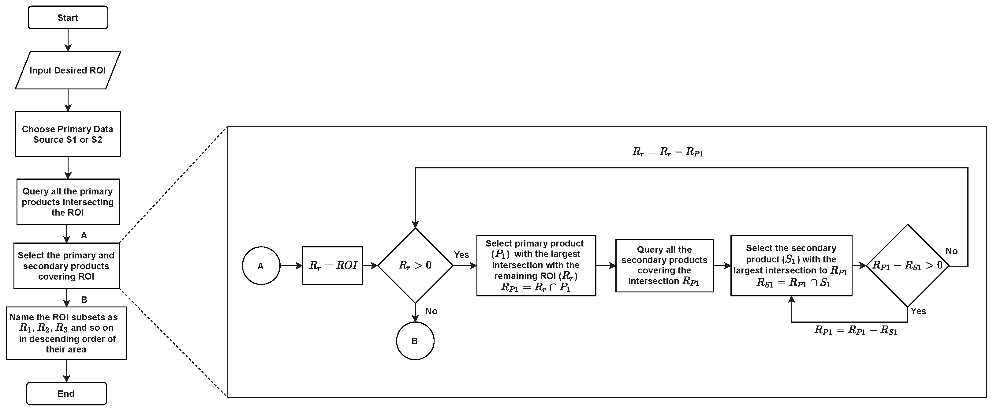
The scene discovery algorithm, shown in Figure 2, starts with the selection of an ROI and the required temporal frequency. The subsequent step is the process of selecting Sentinel products for every date in the time sequence. The selection of the option to obtain Sentinel-1 and Sentinel-2 pairs that cover the target ROI depends on which of the two data sources is considered the primary and secondary satellite, the latter being configurable by the user. The Sentinelsat API queries the Copernicus Data Hub for the metadata on all Sentinel products intersecting with the ROI, including footprints, date of acquisition and percentage of cloud cover within the given temporal duration. The footprint is then used to select the primary product (P1) with the largest overlap to the target ROI, (Rr), resulting in an intersection (RP1). Subsequently, all secondary products (S1) overlapping with RP1 and with close temporal match are queried; the largest secondary product RS1 is selected. Secondary products are searched again until the complete RP1 area is covered. The next primary product is then selected to cover the remaining part of the ROI (Rr-RP1). The process is repeated iteratively until all the target ROI is covered. Finally, all subsets of the ROI are collected and then rearranged in descending order of the overlapping area with the target ROI and named R1, R2, etc. An example of the procedure is illustrated in the case study presented in Section 3.1.

2.3. Data Download and Access

A list of the generated products is forwarded to the download stage on the completion of the scene discovery stage. The framework can ingest data from various data sources, thus enabling instantaneous access to products. The Python Sentinelsat API [46] can query and download data from the Copernicus Open Access Hub [47]. However, the retention policy mandates shifts of old data from the online archive to the Long-Term Archive (LTA); the retention period is 18 months for Copernicus Sentinel-2 L2A. Older products in the LTA can only be accessed upon a trigger generated by a request for each individual product 24 h in advance. The framework implements data retrieval from other platforms that mirror the Copernicus hub, such as the Alaska Satellite Facility (ASF) for Sentinel-1 [48], Google Cloud Storage for Sentinel-2 [49] and Amazon Web Services (AWS) for Sentinel-1 and Sentinel-2 [50,51], limiting the delay for obtaining data. Authentication of the right to access is required from Copernicus, Google Cloud, AWS or ASF to initiate downloading. The downloading stage implements the caching of products to prevent re-downloads of existing products, a considerable time-consuming step.

2.4. Processing Pipelines

The batch processing of Sentinel products is accomplished using the Graph Processing Tool of the ESA SNAP toolbox [39]. The following sections present the processing pipeline for Sentinel-1 and Sentinel-2 products, their collocation, patch creation and output generation. The processing graph described here is provided with the ARD framework; however, custom processing graphs can also be defined, in recognition that applications have the need to alter the processing and its parameters. For instance, there may be a need to disable speckle filtering, change the speckle filtering kernel size or modify calibration or collocation procedures and parameters.
Sentinel-1 products are distributed in the World Geodetic System coordinate reference system, namely the WGS84 (EPSG:4326), whereas the Universal Transverse Mercator (UTM) coordinate system is used by default for Sentinel-2 products. The UTM coordinate system divides the Earth into 60 zones, each 6° wide in longitude and 8° in latitude, transforming the latitude and longitude from the spherical coordinate system to specific zone numbers with corresponding x and y coordinates. The UTM system is preserved for Sentinel-2 products and also followed by Sentinel-1 products through a projection from WGS84 to the corresponding UTM zone, thus maintaining consistency between products.

2.4.1. Sentinel-1 Product Processing

Sentinel-1 products must be processed before they are analysis-ready [52]. The framework adopts a standard processing workflow for GRD products [53] and best practices for the preparation of Sentinel-1 SAR data for the data cube [54]. Informed by reported work, the processing pipeline for Sentinel-1 products implemented in the framework is shown in Figure 3. The Level-1 GRD product must be radiometrically calibrated so that acquisitions captured on different dates can be compared with consideration of the global incidence angle, converting the radar backscatter intensity to the normalised radar cross-section ( σ 0 ). SAR data are impacted by ‘salt-and-pepper’ speckle noise and, although speckle filtering is not a requirement for ARD [40], it is nevertheless performed on the calibrated normalised radar cross-section to minimise further post-processing. Speckle filtering is performed using a Lee-Sigma filter with a window size of 7 × 7, σ of 0.9 and target window size of 3 × 3 [55]. Range Doppler terrain correction is then executed using a Shuttle Radar Topography Mission Height (SRTM) 1 sec HGT Digital Elevation Model (DEM) [56] to remove geometric distortions such as foreshortening, layover and shadow. For illustration, the evolution of the VV band of SAR data through the different stages of the pipeline is shown in Figure 4. The final two steps in the Sentinel-1 processing pipeline are clipping to the required area and the band extractor operation, which selects the bands required in the final product. The cropping of the satellite image to the ROI is implemented in two steps; the subset operator in SNAP crops the tile to the bounds of the ROI to bring down the size of the raster file and reduce the processing time in SNAP, followed by cropping of the image to the exact cut-line of the ROI using the Python Geospatial Data Abstraction Library (GDAL) [57].

2.4.2. Sentinel-2 Product Processing

The processing pipeline for Sentinel-2 products is shown in Figure 5 and follows the procedure recommended by ESA [58]. Sentinel-2 products contain different bands at different spatial resolutions of 10 m, 20 m and 60 m and consequently re-sampling is required to harmonise all bands to the same spatial resolution of 10 m. Masks are obtained from the original product using the BandMaths operator and merged with the re-sampled product using the BandMerge operator. Similarly to the Sentinel-1 processing pipeline, a subset operation in SNAP performs the cropping. The configurable bands are passed as parameters to the band extractor operator to only select the bands and masks required by the user.

2.4.3. Collocation of Sentinel-1 and Sentinel-2 Products

Similar processing steps are followed with the addition of the collocation step when the framework is configured to produce Sentinel-1 and Sentinel-2 pairs; the processing pipeline for collocated Sentinel-1 and Sentinel-2 products is shown in Figure 6. The collocation with bilinear interpolation is performed within the ESA SNAP toolbox by selecting Sentinel-2 as the master product and retaining the UTM projection to maintain the accurate pixel-level alignment between neighbouring tiles required for mosaicking. Collocated tiles are cropped to the boundary of the ROI.

2.5. Patch Creation and Output

The final step in the proposed ARD framework is the creation of patches that are appropriate for input to ML and DL workflows. The ARD framework permits configurations with bespoke patch sizes and overlap between patches in the horizontal and vertical directions. The output pair images are created in a GeoTIFF format containing the bands and masks selected by the user.

2.6. Docker and Parallel Processing

The pipeline, structured around the Metaflow [59] Python framework for the design and management of data science projects, ensures that the multiple steps required to process each satellite product are carried out in the correct order, whilst providing the flexibility to allow end users to extend the framework to shape the ARD for a particular application. Where tasks are able to be processed independently—such as the calibration, filtering and terrain correction of each Sentinel-1 product, or the collocation of matching Sentinel-1 and Sentinel-2 products—the framework can scale horizontally, to fully utilize computing resources and reduce the required processing time, i.e., tasks will be deployed in parallel across each available CPU core.
The generation of ARD is characterised by a number of dependencies. Data sources must be queried, data downloaded, images processed and collocated and optionally cut into separate patches of suitable size for specific applications, e.g., training ML models. The framework specifies all dependencies via a Dockerfile, which can be created and deployed using Docker [60], provisioning a consistent environment managing all necessary dependencies for the preparation of ARD. Docker images are suitable for use on either a personal or office-scale computing infrastructure, and can be readily converted to container images suitable for deployment on a high-performance computing (HPC) infrastructure, such as Singularity [61].

3. Results

A case study showing the generation of combined Sentinel-1 and Sentinel-2 ARD for a region in Scotland is presented for the purposes of providing evidence of the functionality and ease of use of the framework. Inherent challenges in Sentinel products and framework optimisations are then discussed, including the selection of Sentinel-2 products based on local cloud coverage criteria and the avoidance of “no-data” regions at the boundary of Sentinel-1 products. Furthermore, the effect of tile overlaps and an example of the application of the proposed ARD framework to crop monitoring are detailed.

3.1. Case Study: ARD Generation

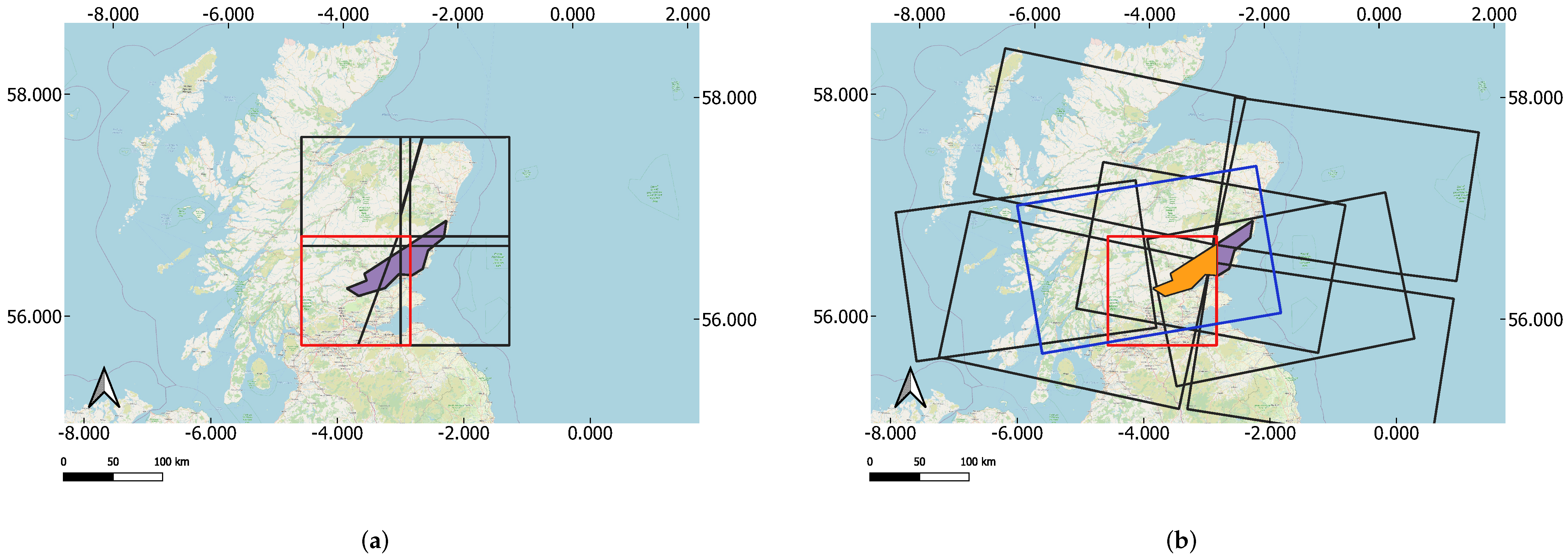
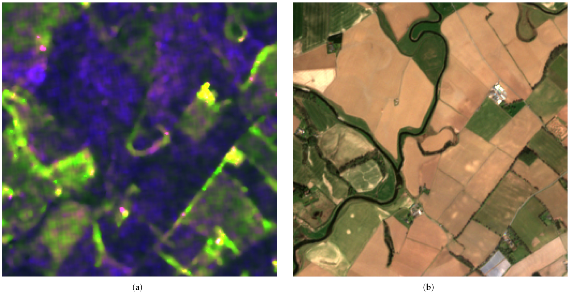
The framework is exercised for a number of locations around the globe to generate collocated multi-modal and multi-temporal data, showcasing the automated end-to-end pipeline. The user can secure Sentinel-1 and Sentinel-2 ARD by specifying the required ROI and time window; for the case study, a region in Scotland, UK, shown in Figure 7, has been selected. The primary product was set as Sentinel-2 and, as a consequence, Sentinel-2 products intersecting with the ROI (violet) are discovered first and the largest product selected (red box), as shown in Figure 7a. After the selection of the primary product is completed (in this case, Sentinel-2), the secondary Sentinel-1 product (blue box) is selected for the above primary product, as shown in Figure 7b. Note that other candidate Sentinel-1 products are not selected either because they do not cover the ROI or because their time difference with the primary Sentinel-2 product is greater. The remaining primary products and their corresponding secondary products are subsequently selected in decreasing order of their intersection area with the ROI. All subsets of the ROI are collected in this manner, shown in Table 1. Figure 8 shows the result of the entire scene discovery process and, in particular, illustrates (a) all Sentinel-2 segments that cover the ROI and (b) and (c) the Sentinel-1 and Sentinel-2 mosaics for the target ROI. Both mosaics, as they are now collocated, can be segmented in patches to create pairs, as shown in Figure 9. Image pairs are analysis-ready—for example, aligned with the needs of developing ML algorithms for downstream services and for further analysis.

3.2. Challenges and Optimisations

Examples of the manner in which the framework treats a number of challenges in building ARD data, particularly cloud cover and “no-data” regions at the boundary of Sentinel-1 products, are described as additional evidence of its utility.

3.2.1. Sentinel-2 Product Selection Based on Cloud Criteria

A number of applications that make use of satellite imagery, such as land cover classification, crop identification or crop growth monitoring, are founded on cloud-free optical images for operation.
The degree of cloud coverage—referred to as the cloud fraction—is measured as the ratio of the area covered by the cloud (irrespective of cloud type) to the total observed area. The global cloud cover fraction can be estimated by the analysis of satellite images or by using synoptic reports taken from ground-based weather stations. The average global cloud cover fraction has been calculated—based on data retrieved from 12 satellite image datasets—to be 68% for clouds of optical depth greater than 0.1, increasing to 72% when sub-visible cirrus clouds are also considered [62]. The global cloud fraction as determined by the Moderate Resolution Imaging Spectroradiometer (MODIS) sensor from the Terra and Aqua satellites is 67%, with lower cloud coverage in land areas (55%) than over the ocean (72%) [63].
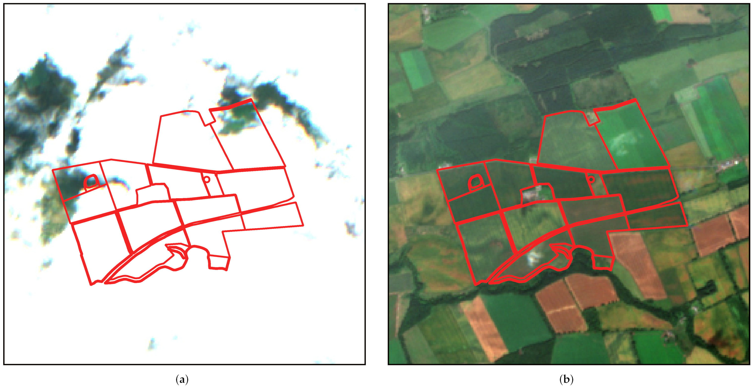
The creation of a minimum cloud-free mosaic for Sentinel-2 optical images is a challenge for areas subject to significant cloud cover, necessitating the strategic selection of tiles. The least cloud-affected tile must be chosen among all the tiles covering a particular ROI within the given time window. Ideally, the cloud fraction should be assessed during the initial selection of the tiles to avoid unnecessary downloads and processing. Sentinel-2 products contain information on the degree of cloud cover evaluated over the entire tile. However, the cloud cover for a particular ROI cannot be determined from tile information alone. In instances where the ROI is cloud-free while the rest of the tile is not, the latter will not be selected if only the average cloud cover statistics are considered. As an example, the tile captured on 21 July 2020 is 19.24% cloud-covered, as shown in Figure 10 for a group of farms in Scotland; however, closer inspection shows significant cloud cover over the ROI (Figure 10a). For a tile captured two days later, on 23 July 2020, the cloud coverage is 90.83% but the ROI is cloud-free (Figure 10b). Therefore, accurate per-pixel metadata are required to guide the tile selection process based on cloud coverage.
In the proposed framework, Sentinel-2 Level-2A scene classification masks (cloud medium probability, cloud high probability, thin cirrus) are downloaded to determine the exact cloud-free area over the ROI. The resultant outputs inform the selection of tiles with minimum cloud coverage, and thus situations such as the one presented in Figure 10 are avoided. In addition, other scene classification masks can be used for semantic enrichment, providing additional information on the presence of vegetation, snow, water, cloud shadows, etc.

3.2.2. “No-Data” Values in Sentinel-1 Products

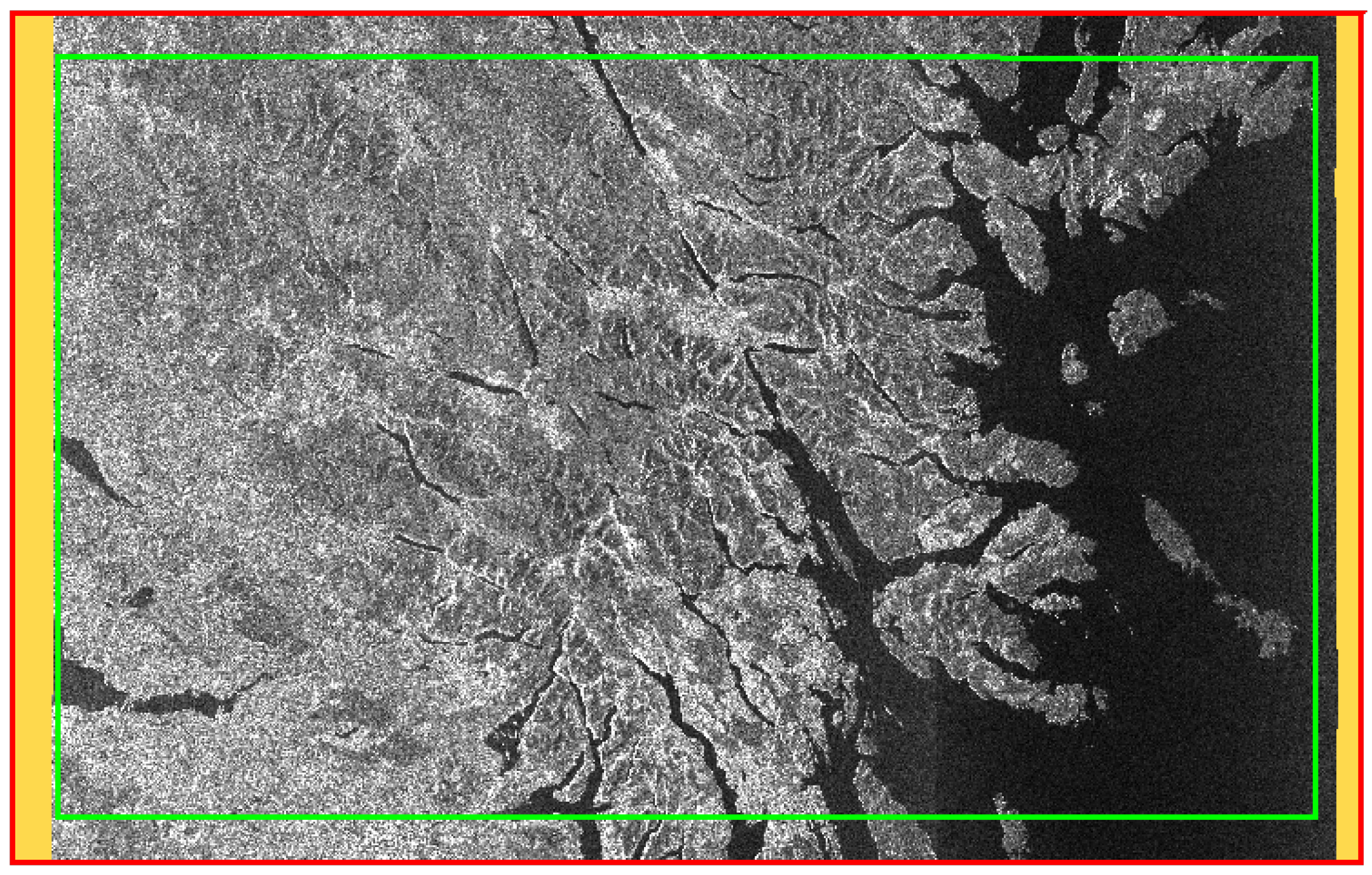
The Sentinel-1 product footprint is used for the selection of tiles covering the ROI, performed prior to downloading products so that only the required data are obtained and processed. However, the footprint provided by the Copernicus product can be larger than the region where data are present, creating a margin of “no-data” values at the boundary of the product, as shown by the yellow region in Figure 11. The mismatch between the original footprint and the region where data are available can lead to the erroneous selection of products when the ROI overlaps with the “no-data” region. One potential solution is to download all the Sentinel-1 products intersecting with the ROI and to process them with the SNAP pipeline to determine the exact footprint. However, this option increases both the download and processing time and memory requirements significantly. Thus, the framework introduces a buffered boundary inside the original footprint, as shown in green in Figure 11, which is then used for the selection of products. The latter approach implements faster product selection, while ensuring that only regions where data are available are downloaded and processed.

3.3. Effect of Tile Overlap

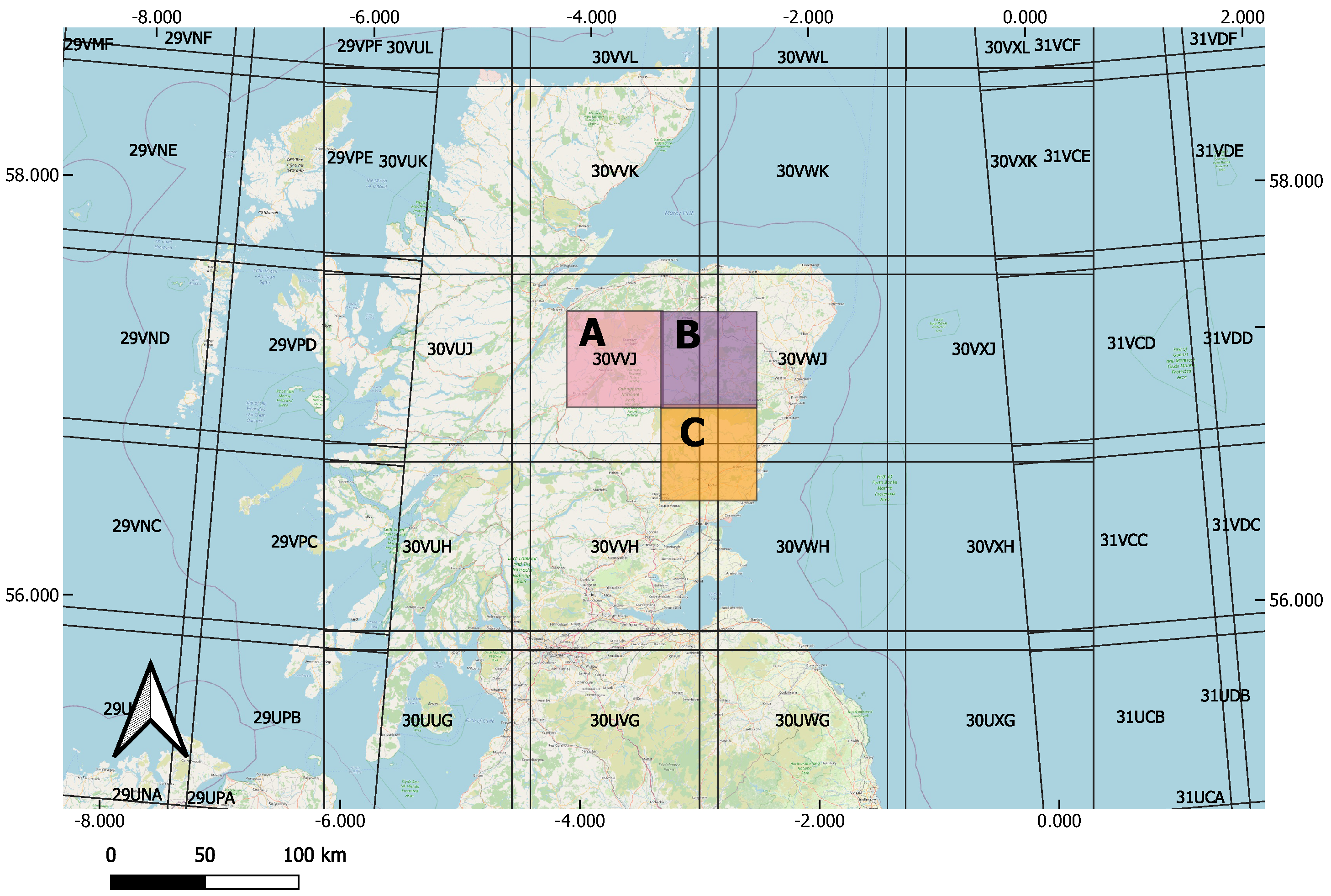
The required number of tiles necessary to fully cover the region varies depending on the location of the target ROI. A case study for an ROI of approximately 51.2 km × 51.2 km in Scotland for the week from the 3 May 2021 to the 9 May 2021 is analysed to give an indication of the processing times required by the framework to generate multi-modal ARD as a function of the required number of tiles for full coverage. Sentinel-2 products are available in pre-defined tiles of approximately 100 km × 100 km area and 800 MB file size [45], with each tile assigned a unique identifier [64]. In this case study, three ROIs of equal area are defined, A, B and C, as shown in Figure 12, spanning one, two and four tiles, respectively, dependent on their location on the Sentinel-2 tile grid. Each Sentinel-2 product could require multiple Sentinel-1 products to generate paired ARD patches. The framework is executed for scene discovery, download and processing of Sentinel-1 and Sentinel-2 products. Both the VV and VH polarization bands are downloaded and processed for Sentinel-1, while, for Sentinel-2, all spectral bands in Level-2A, along with opaque cloud, cirrus cloud and scene classification masks for cloud shadow and medium- and high-probability thin cirrus, are downloaded and processed. The patch size is set to 256 × 256 pixels.
The framework is executed on a 10-physical-core CPU (Intel i9-10900X) Linux server with 126 GB RAM and 9 TB storage. The time required to produce multi-modal ARD for the three scenarios, i.e., A, B, C, is shown in Table 2. The selection time includes the time for querying products using the Sentinelsat API and selecting Sentinel-1 and Sentinel-2 products using the scene discovery algorithm, as discussed in Section 2.2. The processing time includes the processing for Sentinel-1 and Sentinel-2 products, collocation using the SNAP GPT and the creation of patches, as described in Section 2.4. The total time is the aggregate of selection and processing times. The download time is not considered due to the variability of network connections and data provider. As shown in Table 2, the time for processing increases if the ROI falls within the boundaries of the Sentinel-2 tile grid, attributable to the increased number of tile pairs processed. However, the processing time does not scale linearly, due to the varying number of overlapping segments for each collocation.

3.4. Application: Multi-Modal and Multi-Temporal ARD for Crop Monitoring

Vegetation has been proven to strongly absorb the blue and red bands of the visible segment of the electromagnetic spectrum and reflect the near-infrared wavelengths [65]; these characteristics form the basis for the detection of vegetation on the surface of the Earth from satellite sensor data. The Normalised Difference Vegetation Index (NDVI) [66], calculated as the ratio of the difference in reflectance between the near-infrared and the red band to the sum of reflectance between the near-infrared and the red band, as shown in Equation (1), has been defined in this context:
N D V I = N I R R E D N I R + R E D
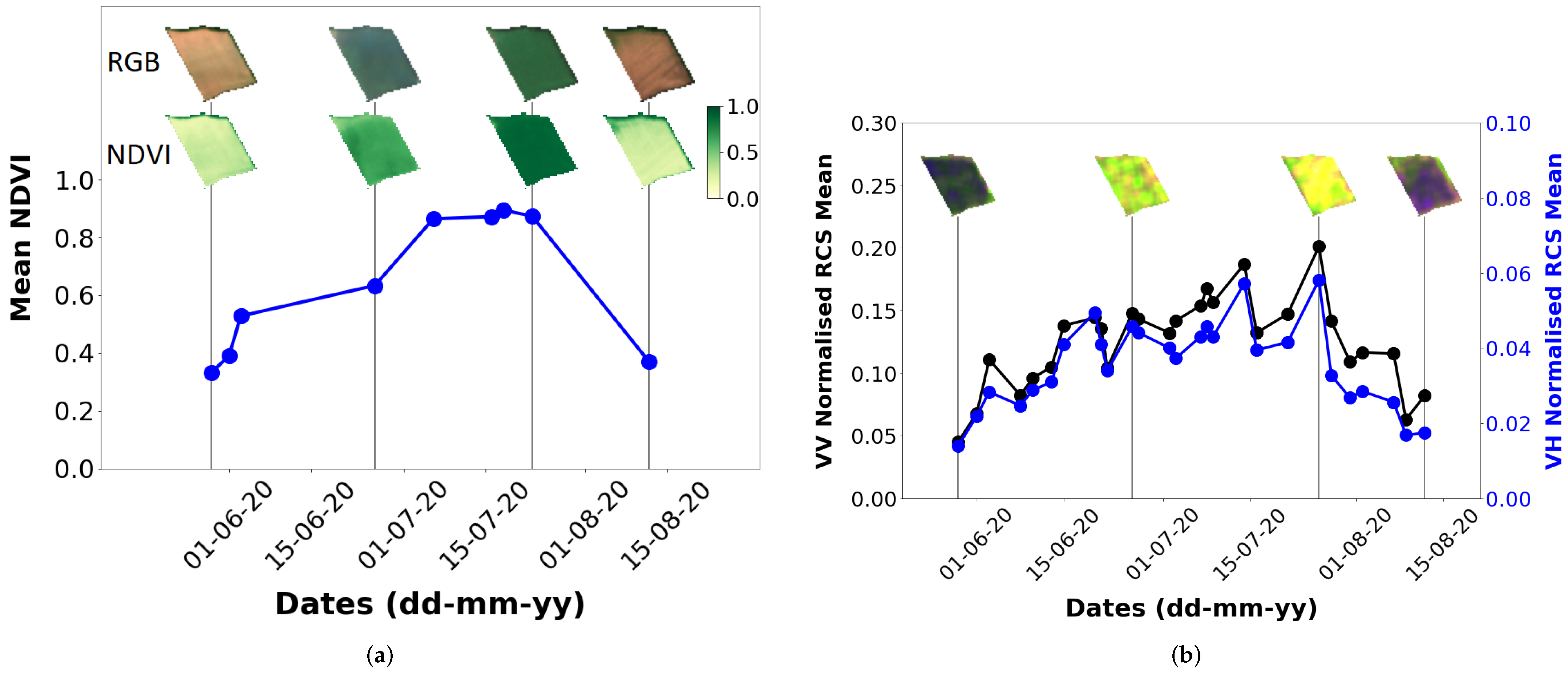
The NDVI ranges from −1 to 1, with negative values indicating clouds and water, positive values close to 0 corresponding to no vegetation and dense vegetation corresponding to a value close to 1. The NDVI has been used to monitor the growth of crops and for the estimation of crop yield [67,68]. An example of the variation of NDVI for a field of peas in Scotland for the period of 29 May 2020 to 12 August 2020 is shown in Figure 13. Figure 13a shows the time series of the mean NDVI along with sample RGB and NDVI cloud-free images; Figure 13b shows the mean of SAR VV and VH polarisation normalised radar cross-section (RCS) along with Sentinel-1 false colour composite images for the field for all available acquisitions in the period. Evident in Figure 13a is that NDVI values are lower before sowing (May–June 2020), viz. when the soil is bare, and after harvest (August 2020); the NDVI increases with crop growth (July–August 2020). A similar trend can be observed in the SAR data shown in Figure 13b, illustrating the potential to facilitate further studies in these applications that combine Sentinel-1 and Sentinel-2 data [69,70,71].

4. Conclusions

The pairing of Sentinel-1 and Sentinel-2 data and the use of their complementary information has considerable potential in a wide range of applications, including land cover classification, crop growth monitoring and deforestation mapping. However, the generation of reliable multi-modal and multi-temporal ARD from low-level Sentinel products remains a challenge. Here, a flexible, user-centric framework is introduced for the on-demand selection, download and processing of Sentinel-1 and Sentinel-2 data for a user-defined ROI and time window. The tool can be configured to meet specific user requirements, enabling rapid access to combined ARD for downstream applications with global coverage. The framework is built in Python and containerised using Docker to ensure a consistent environment treating all necessary dependencies.
The framework selects the minimum number of satellite tiles required to cover a particular ROI within a specific timeframe, optimising the time-consuming process of downloading Sentinel products. Furthermore, when multi-source data are required, the framework follows a standard pipeline for processing Sentinel-1—radiometric calibration, speckle filtering, terrain correction—and Sentinel-2—re-sampling—products, the subsequent collocation of these products and their clipping to the shape of the ROI. Additionally, challenges inherent to Sentinel data, such as the presence of “no-data” regions in Sentinel-1 products and a more appropriate selection of Sentinel-2 products based on local cloud masks instead of tile-level cloud percentages, are addressed. The ability to generate time series of collocated Sentinel-1 and Sentinel-2 ARD is demonstrated, providing further insight to users through time-dependent trends relevant to specific applications, e.g., crop growth monitoring.
The current version of the framework is applicable to Sentinel-1 GRD products that provide radar backscatter amplitude; however, it could be extended to include Sentinel-1 Level-1 Single Look Complex (SLC) products; the latter’s intrinsic phase information can be useful in applications such as land cover mapping and crop monitoring, which rely on interferometric coherence to detect changes in the SAR signal. Moreover, the framework could be extended to include data from other Sentinel missions, providing a wider variety of EO ARD, such as Sentinel-3 data relevant to marine observation and land monitoring, and Sentinel-4 and Sentinel-5 data enabling the potential to monitor air quality.

Author Contributions

Conceptualization, C.T., J.C. and I.A.; methodology, P.U., M.C. and C.D.; software, P.U., C.D. and N.P.; validation, J.C., N.P. and R.A.; investigation, P.U. and M.C.; data curation, P.U., M.C. and C.D.; writing—original draft preparation, P.U., M.C., C.D. and J.C.; writing—review and editing, M.M., I.A., C.M., R.A., K.N. and C.T.; visualization, P.U. and C.D.; supervision, J.C., M.M., I.A., C.M., R.A. and C.T.; project administration, I.A., C.M. and C.T.; funding acquisition, I.A., C.M., R.A. and C.T. All authors have read and agreed to the published version of the manuscript.

Funding

This research was funded by the European Union Horizon 2020 research and innovation programme, grant number 825355.

Institutional Review Board Statement

Not applicable.

Informed Consent Statement

Not applicable.

Data Availability Statement

Publicly available Sentinel-1 and Sentinel-2 data products used in this study can be found at: https://scihub.copernicus.eu/, accessed on 31 January 2022.

Acknowledgments

The work was partially funded by European Union Horizon 2020 research and innovation programme “Fostering Precision Agriculture and Livestock Farming through Secure Access to Large-Scale HPC-Enabled Virtual Industrial Experimentation Environment Empowering Scalable Big Data Analytics (H2020-ICT-2018-2020) (CYBELE)” under the grant agreement NO. 825355.

Conflicts of Interest

The authors declare no conflict of interest. The funders had no role in the design of the study; in the collection, analyses, or interpretation of data; in the writing of the manuscript, or in the decision to publish the results.

Appendix A

Appendix A.1. Naming Convention
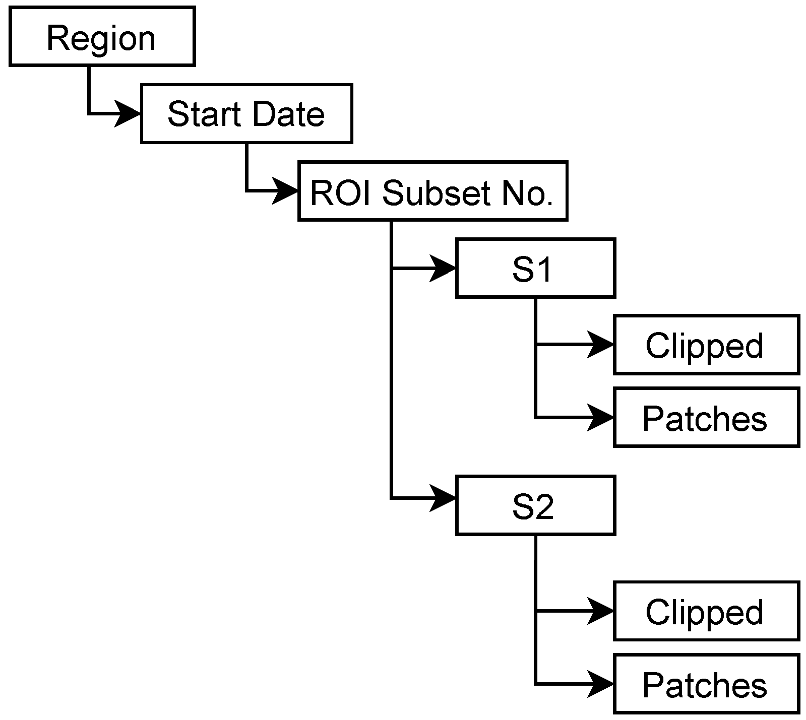
The framework adopts a consistent naming convention and folder structure, as shown in Figure A1. Sentinel-1 and Sentinel-2 data are stored in the S1 and S2 folder, respectively, and contain the ROI in the Clipped folder and the corresponding patches in the Patches folder. S1_id and S2_id are the universally unique identifiers (UUIDs) for Sentinel-1 and Sentinel-2, respectively. ROI subsets are numbered in descending order to their overlapped area with the region of interest, i.e., ROI1 is the Sentinel-2 tile that has the largest intersection with the ROI and so on. start_row_px and start_col_px are the top left corner row and column pixel numbers for the cropped patches of the ROI, and row_size and col_size are the number of pixels in the patch for the rows and columns, respectively. The clipped Sentinel-1 tiles are stored in the following manner:
S1_roi<ROI_no>_<S1_id>.tif
For instance,
S1_roi1_2c522712-e4a5-4bec-a828-4c8d5c0930f4.tif
The generated Sentinel-1 patches are stored in the following manner:
S1_<S1_id>_<start_row_px>_<start_col_px>_<row_size>x<col_size>.tif
For instance,
S1_2c522712-e4a5-4bec-a828-4c8d5c0930f4_0_0_256x256.tif
The generated Sentinel-2 patches are stored following similar naming conventions as Sentinel-1. For collocated Sentinel-1 and Sentinel-2, the patches follow the naming convention shown below.
S1_<S1_id>_S2_<S2_id>_<start_row_px>_<start_col_px>_<row_size>x<col_size>.tif
For instance,
S1_2c522712-e4a5-4bec-a828-4c8d5c0930f4_S2_8a9cbfaa-1a59-4dd4-ad28-5ee48cc5866e_0_0_256x256.tif
Figure A1. Folder structure.
Remotesensing 14 01120 g0a1

Appendix A.2. Configuration Parameters

Table A1. Parameters used in configuration of the ARD Framework.
ParameterDescription
NameThis will set the name of the folder as per convention mentioned in Appendix A.
datesPair of dates (in format YYYYMMDD) specifying the start and end of the period of interest.
geojsonGeojson string representing the ROI.
cloudcoverPair of integers (in range 0..100) specifying lower and upper threshold for cloud cover at the tile level for queries of Sentinel-2 products.
cloud mask filteringThis option is set to build maximum cloud-free Sentinel-2 image based on per pixel cloud mask from scene classification mask.
sizePair of integers specifying the row and column size, in pixels, of patch to generate.
overlapPair of integers specifying the horizontal and vertical overlap between patches, where 0 indicates no overlap, while 1 indicates maximum overlap.
bands_S1The polarization bands required for Sentinel-1 GRD products.
bands_S2The multi-spectral and mask bands required for Sentinel-2 Level-2A products.
callback_snapConfigurable function used to run custom processing for each set of (potentially) multi-modal, multi-temporal products.
callback_find_productsConfigurable function used to identify sets of multi-modal, multi-temporal products.
Table A2. Parameters used for ARD framework run-time.
ParameterDescription
RebuildThis will delete any earlier processed products and rebuild the processed products.
Skip weekThis will skip all weeks that do not yield products covering complete ROI.
Primary productThis option will select primary product as Sentinel-1 or Sentinel-2. The default primary product is set as Sentinel-2. The secondary products are selected around the primary product within the “Secondary Time Delta” days.
Skip secondaryThis will skip the listing and processing of secondary product. This option is used when only one out of Sentinel-1 or Sentinel-2 products is relevant.
External BucketThis will check for Long-Term Archived (LTA) products from AWS, Google, Sentinelhub, ASF.
Available areaThis option will list part of an ROI that matches the required specifications, even if the whole ROI is not available.
Secondary Time DeltaThis option specifies the delta time between primary and secondary products in days.
Primary product frequencyThis option selects the frequency in days between primary products.

References

  1. Anderson, K.; Ryan, B.; Sonntag, W.; Kavvada, A.; Friedl, L. Earth observation in service of the 2030 Agenda for Sustainable Development. Geo-Spat. Inf. Sci. 2017, 20, 77–96. [Google Scholar] [CrossRef]
  2. Schumann, G.J.P.; Brakenridge, G.R.; Kettner, A.J.; Kashif, R.; Niebuhr, E. Assisting Flood Disaster Response with Earth Observation Data and Products: A Critical Assessment. Remote Sens. 2018, 10, 1230. [Google Scholar] [CrossRef] [Green Version]
  3. Guzinski, R.; Kass, S.; Huber, S.; Bauer-Gottwein, P.; Jensen, I.H.; Naeimi, V.; Doubkova, M.; Walli, A.; Tottrup, C. Enabling the Use of Earth Observation Data for Integrated Water Resource Management in Africa with the Water Observation and Information System. Remote Sens. 2014, 6, 7819–7839. [Google Scholar] [CrossRef] [Green Version]
  4. Bouvet, A.; Mermoz, S.; Ballère, M.; Koleck, T.; Le Toan, T. Use of the SAR Shadowing Effect for Deforestation Detection with Sentinel-1 Time Series. Remote Sens. 2018, 10, 1250. [Google Scholar] [CrossRef] [Green Version]
  5. Wangchuk, S.; Bolch, T. Mapping of glacial lakes using Sentinel-1 and Sentinel-2 data and a random forest classifier: Strengths and challenges. Sci. Remote Sens. 2020, 2, 100008. [Google Scholar] [CrossRef]
  6. Gargiulo, M.; Dell’Aglio, D.A.G.; Iodice, A.; Riccio, D.; Ruello, G. Integration of Sentinel-1 and Sentinel-2 Data for Land Cover Mapping Using W-Net. Sensors 2020, 20, 2969. [Google Scholar] [CrossRef]
  7. Orynbaikyzy, A.; Gessner, U.; Mack, B.; Conrad, C. Crop Type Classification Using Fusion of Sentinel-1 and Sentinel-2 Data: Assessing the Impact of Feature Selection, Optical Data Availability, and Parcel Sizes on the Accuracies. Remote Sens. 2020, 12, 2779. [Google Scholar] [CrossRef]
  8. Meraner, A.; Ebel, P.; Zhu, X.X.; Schmitt, M. Cloud removal in Sentinel-2 imagery using a deep residual neural network and SAR-optical data fusion. ISPRS J. Photogramm. Remote Sens. 2020, 166, 333–346. [Google Scholar] [CrossRef]
  9. Gao, Q.; Zribi, M.; Escorihuela, M.J.; Baghdadi, N. Synergetic Use of Sentinel-1 and Sentinel-2 Data for Soil Moisture Mapping at 100 m Resolution. Sensors 2017, 17, 1966. [Google Scholar] [CrossRef] [Green Version]
  10. Huang, L.; Liu, B.; Li, B.; Guo, W.; Yu, W.; Zhang, Z.; Yu, W. OpenSARShip: A Dataset Dedicated to Sentinel-1 Ship Interpretation. IEEE J. Sel. Top. Appl. Earth Obs. Remote Sens. 2018, 11, 195–208. [Google Scholar] [CrossRef]
  11. Zhao, J.; Zhang, Z.; Yao, W.; Datcu, M.; Xiong, H.; Yu, W. OpenSARUrban: A Sentinel-1 SAR Image Dataset for Urban Interpretation. IEEE J. Sel. Top. Appl. Earth Obs. Remote Sens. 2020, 13, 187–203. [Google Scholar] [CrossRef]
  12. Ardö, J. A Sentinel-2 Dataset for Uganda. Data 2021, 6, 35. [Google Scholar] [CrossRef]
  13. Helber, P.; Bischke, B.; Dengel, A.; Borth, D. Introducing Eurosat: A Novel Dataset and Deep Learning Benchmark for Land Use and Land Cover Classification. In Proceedings of the IGARSS 2018—2018 IEEE International Geoscience and Remote Sensing Symposium, Valencia, Spain, 22–27 July 2018; pp. 204–207. [Google Scholar] [CrossRef]
  14. Weikmann, G.; Paris, C.; Bruzzone, L. TimeSen2Crop: A Million Labeled Samples Dataset of Sentinel 2 Image Time Series for Crop-Type Classification. IEEE J. Sel. Top. Appl. Earth Obs. Remote Sens. 2021, 14, 4699–4708. [Google Scholar] [CrossRef]
  15. Schmitt, M.; Hughes, L.H.; Zhu, X.X. The SEN1-2 dataset for deep learning in SAR-optical data fusion. ISPRS Ann. Photogramm. Remote Sens. Spat. Inf. Sci. 2018, IV-1, 141–146. [Google Scholar] [CrossRef] [Green Version]
  16. Schmitt, M.; Hughes, L.; Qiu, C.; Zhu, X. SEN12MS—A Curated Dataset of Georeferenced Multi-Spectral Sentinel-1/2 Imagery for Deep Learning and Data Fusion. arXiv 2019, arXiv:1906.07789. [Google Scholar] [CrossRef] [Green Version]
  17. Zhu, X.X.; Hu, J.; Qiu, C.; Shi, Y.; Kang, J.; Mou, L.; Bagheri, H.; Haberle, M.; Hua, Y.; Huang, R.; et al. So2Sat LCZ42: A Benchmark Data Set for the Classification of Global Local Climate Zones [Software and Data Sets]. IEEE Geosci. Remote Sens. Mag. 2020, 8, 76–89. [Google Scholar] [CrossRef] [Green Version]
  18. Augustin, H.; Sudmanns, M.; Tiede, D.; Lang, S.; Baraldi, A. Semantic Earth Observation Data Cubes. Data 2019, 4, 102. [Google Scholar] [CrossRef] [Green Version]
  19. Lewis, A.; Oliver, S.; Lymburner, L.; Evans, B.; Wyborn, L.; Mueller, N.; Raevksi, G.; Hooke, J.; Woodcock, R.; Sixsmith, J.; et al. The Australian Geoscience Data Cube—Foundations and lessons learned. Remote Sens. Environ. 2017, 202, 276–292. [Google Scholar] [CrossRef]
  20. Lewis, A.; Lymburner, L.; Purss, M.B.J.; Brooke, B.; Evans, B.; Ip, A.; Dekker, A.G.; Irons, J.R.; Minchin, S.; Mueller, N.; et al. Rapid, high-resolution detection of environmental change over continental scales from satellite data – the Earth Observation Data Cube. Int. J. Digit. Earth 2016, 9, 106–111. [Google Scholar] [CrossRef]
  21. Giuliani, G.; Chatenoux, B.; Bono, A.D.; Rodila, D.; Richard, J.P.; Allenbach, K.; Dao, H.; Peduzzi, P. Building an Earth Observations Data Cube: Lessons learned from the Swiss Data Cube (SDC) on generating Analysis Ready Data (ARD). Big Earth Data 2017, 1, 100–117. [Google Scholar] [CrossRef] [Green Version]
  22. Giuliani, G.; Chatenoux, B.; Honeck, E.; Richard, J.P. Towards Sentinel-2 Analysis Ready Data: A Swiss Data Cube Perspective. In Proceedings of the IGARSS 2018—2018 IEEE International Geoscience and Remote Sensing Symposium, Valencia, Spain, 22–27 July 2018; pp. 8659–8662. [Google Scholar] [CrossRef] [Green Version]
  23. Ariza Porras, C.; Bravo, G.; Villamizar, M.; Moreno, A.; Castro, H.; Galindo, G.; Cabera, E.; Valbuena, S.; Lozano-Rivera, P. CDCol: A Geoscience Data Cube that Meets Colombian Needs. In Colombian Conference on Computing; Springer: Cham, Switzerland, 2017; pp. 87–99. [Google Scholar] [CrossRef]
  24. Cheng, M.C.; Chiou, C.R.; Chen, B.; Liu, C.; Lin, H.C.; Shih, I.L.; Chung, C.H.; Lin, H.Y.; Chou, C.Y. Open Data Cube (ODC) in Taiwan: The Initiative and Protocol Development. In Proceedings of the IGARSS 2019—2019 IEEE International Geoscience and Remote Sensing Symposium, Yokohama, Japan, 28 July–2 August 2019; pp. 5654–5657. [Google Scholar] [CrossRef]
  25. Dhu, T.; Dunn, B.; Lewis, B.; Lymburner, L.; Mueller, N.; Telfer, E.; Lewis, A.; McIntyre, A.; Minchin, S.; Phillips, C. Digital earth Australia – unlocking new value from earth observation data. Big Earth Data 2017, 1, 64–74. [Google Scholar] [CrossRef] [Green Version]
  26. Digital Earth Africa (DE Africa). Available online: https://www.earthobservations.org/documents/gwp20_22/DE-AFRICA.pdf (accessed on 5 October 2021).
  27. Ticehurst, C.; Zhou, Z.S.; Lehmann, E.; Yuan, F.; Thankappan, M.; Rosenqvist, A.; Lewis, B.; Paget, M. Building a SAR-Enabled Data Cube Capability in Australia Using SAR Analysis Ready Data. Data 2019, 4, 100. [Google Scholar] [CrossRef] [Green Version]
  28. The “Road to 20” International Data Cube Deployments. Available online: https://ecb55191-c6e7-461e-a453-1feef4c7e8b7.filesusr.com/ugd/8959d6_cfcba3751fe642bc9faec776ab98cb20.pdf (accessed on 5 October 2021).
  29. Frantz, D. FORCE—Landsat + Sentinel-2 Analysis Ready Data and Beyond. Remote Sens. 2019, 11, 1124. [Google Scholar] [CrossRef] [Green Version]
  30. Baumann, P.; Mazzetti, P.; Ungar, J.; Barbera, R.; Barboni, D.; Beccati, A.; Bigagli, L.; Boldrini, E.; Bruno, R.; Calanducci, A.; et al. Big Data Analytics for Earth Sciences: The EarthServer approach. Int. J. Digit. Earth 2016, 9, 3–29. [Google Scholar] [CrossRef]
  31. Gorelick, N.; Hancher, M.; Dixon, M.; Ilyushchenko, S.; Thau, D.; Moore, R. Google Earth Engine: Planetary-scale geospatial analysis for everyone. Remote Sens. Environ. 2017, 202, 18–27. [Google Scholar] [CrossRef]
  32. Giuliani, G.; Masó, J.; Mazzetti, P.; Nativi, S.; Zabala, A. Paving the Way to Increased Interoperability of Earth Observations Data Cubes. Data 2019, 4, 113. [Google Scholar] [CrossRef] [Green Version]
  33. Giuliani, G.; Chatenoux, B.; Piller, T.; Moser, F.; Lacroix, P. Data Cube on Demand (DCoD): Generating an earth observation Data Cube anywhere in the world. Int. J. Appl. Earth Obs. Geoinf. 2020, 87, 102035. [Google Scholar] [CrossRef]
  34. Appel, M.; Pebesma, E. On-Demand Processing of Data Cubes from Satellite Image Collections with the gdalcubes Library. Data 2019, 4, 92. [Google Scholar] [CrossRef] [Green Version]
  35. Planque, C.; Lucas, R.; Punalekar, S.; Chognard, S.; Hurford, C.; Owers, C.; Horton, C.; Guest, P.; King, S.; Williams, S.; et al. National Crop Mapping Using Sentinel-1 Time Series: A Knowledge-Based Descriptive Algorithm. Remote Sens. 2021, 13, 846. [Google Scholar] [CrossRef]
  36. El Mendili, L.; Puissant, A.; Chougrad, M.; Sebari, I. Towards a Multi-Temporal Deep Learning Approach for Mapping Urban Fabric Using Sentinel 2 Images. Remote Sens. 2020, 12, 423. [Google Scholar] [CrossRef] [Green Version]
  37. Roy, D.P.; Huang, H.; Boschetti, L.; Giglio, L.; Yan, L.; Zhang, H.H.; Li, Z. Landsat-8 and Sentinel-2 burned area mapping - A combined sensor multi-temporal change detection approach. Remote Sens. Environ. 2019, 231, 111254. [Google Scholar] [CrossRef]
  38. Pinto, M.M.; Libonati, R.; Trigo, R.M.; Trigo, I.F.; DaCamara, C.C. A deep learning approach for mapping and dating burned areas using temporal sequences of satellite images. ISPRS J. Photogramm. Remote Sens. 2020, 160, 260–274. [Google Scholar] [CrossRef]
  39. SNAP. Available online: https://step.esa.int/main/toolboxes/SNAP/ (accessed on 6 October 2021).
  40. Lewis, A.; Lacey, J.; Mecklenburg, S.; Ross, J.; Siqueira, A.; Killough, B.; Szantoi, Z.; Tadono, T.; Rosenavist, A.; Goryl, P.; et al. CEOS Analysis Ready Data for Land (CARD4L) Overview. In Proceedings of the IGARSS 2018—2018 IEEE International Geoscience and Remote Sensing Symposium, Valencia, Spain, 22–27 July 2018; pp. 7407–7410. [Google Scholar] [CrossRef]
  41. CEOS Analysis Ready Data for Land (CARD4L). Available online: https://ceos.org/document_management/Meetings/Plenary/30/Documents/5.5_CEOS-CARD4L-Description_v.22.docx (accessed on 16 November 2021).
  42. Torres, R.; Snoeij, P.; Geudtner, D.; Bibby, D.; Davidson, M.; Attema, E.; Potin, P.; Rommen, B.; Floury, N.; Brown, M.; et al. GMES Sentinel-1 mission. Remote Sens. Environ. 2012, 120, 9–24. [Google Scholar] [CrossRef]
  43. Drusch, M.; Del Bello, U.; Carlier, S.; Colin, O.; Fernandez, V.; Gascon, F.; Hoersch, B.; Isola, C.; Laberinti, P.; Martimort, P.; et al. Sentinel-2: ESA’s Optical High-Resolution Mission for GMES Operational Services. Remote Sens. Environ. 2012, 120, 25–36. [Google Scholar] [CrossRef]
  44. Sentinel Online—Sentinel-2 Level-2A Processing. Available online: https://sentinels.copernicus.eu/web/sentinel/user-guides/sentinel-2-msi/processing-levels/level-2 (accessed on 29 November 2021).
  45. Sentinel Online—Data Products. Available online: https://sentinels.copernicus.eu/web/sentinel/missions/sentinel-2/data-products (accessed on 6 October 2021).
  46. Sentinelsat. Available online: https://sentinelsat.readthedocs.io/en/master/index.html (accessed on 6 October 2021).
  47. Copernicus Open Access Hub. Available online: https://scihub.copernicus.eu/ (accessed on 6 October 2021).
  48. Copernicus Sentinel-1 Data 2018, 2019, 2020. Retrieved from ASF DAAC 28 July 2021, Processed by ESA. Available online: https://asf.alaska.edu/data-sets/sar-data-sets/sentinel-1/sentinel-1-data-and-imagery/ (accessed on 31 January 2022).
  49. Sentinel-2 Data. Available online: https://cloud.google.com/storage/docs/public-datasets/sentinel-2 (accessed on 6 October 2021).
  50. Registry of Open Data on AWS Sentinel-1. Available online: https://registry.opendata.aws/sentinel-1/ (accessed on 6 October 2021).
  51. Registry of Open Data on AWS Sentinel-2. Available online: https://registry.opendata.aws/sentinel-2/ (accessed on 6 October 2021).
  52. SAR Basics Tutorial. Available online: http://step.esa.int/docs/tutorials/S1TBX%20SAR%20Basics%20Tutorial.pdf (accessed on 6 October 2021).
  53. Filipponi, F. Sentinel-1 GRD Preprocessing Workflow. Proceedings 2019, 18, 11. [Google Scholar] [CrossRef] [Green Version]
  54. Truckenbrodt, J.; Freemantle, T.; Williams, C.; Jones, T.; Small, D.; Dubois, C.; Thiel, C.; Rossi, C.; Syriou, A.; Giuliani, G. Towards Sentinel-1 SAR Analysis-Ready Data: A Best Practices Assessment on Preparing Backscatter Data for the Cube. Data 2019, 4, 93. [Google Scholar] [CrossRef] [Green Version]
  55. Lee, J.S.; Wen, J.H.; Ainsworth, T.; Chen, K.S.; Chen, A. Improved Sigma Filter for Speckle Filtering of SAR Imagery. IEEE Trans. Geosci. Remote Sens. 2009, 47, 202–213. [Google Scholar] [CrossRef]
  56. USGS EROS Archive—Digital Elevation—Shuttle Radar Topography Mission (SRTM) 1 Arc-Second Global. Available online: https://www.usgs.gov/centers/eros/science/usgs-eros-archive-digital-elevation-shuttle-radar-topography-mission-srtm-1-arc (accessed on 15 November 2021).
  57. GDAL. Available online: https://pypi.org/project/GDAL/ (accessed on 15 November 2021).
  58. Synergetic Use of Radar and Optical Data. Available online: http://step.esa.int/docs/tutorials/S1TBX%20Synergetic%20use%20127of%20S1%20(SAR)%20and%20S2%20(optical)%20data%20Tutorial.pdf (accessed on 18 October 2021).
  59. Metaflow: A Framework for Real-Life Data Science. Available online: https://metaflow.org/ (accessed on 26 August 2021).
  60. Merkel, D. Docker: Lightweight linux containers for consistent development and deployment. Linux J. 2014, 2014, 2. [Google Scholar]
  61. Kurtzer, G.M.; Sochat, V.; Bauer, M.W. Singularity: Scientific containers for mobility of compute. PLoS ONE 2017, 12, e0177459. [Google Scholar] [CrossRef]
  62. Stubenrauch, C.J.; Rossow, W.B.; Kinne, S.; Ackerman, S.; Cesana, G.; Chepfer, H.; Girolamo, L.D.; Getzewich, B.; Guignard, A.; Heidinger, A.; et al. Assessment of Global Cloud Datasets from Satellites: Project and Database Initiated by the GEWEX Radiation Panel. Bull. Am. Meteorol. Soc. 2013, 94, 1031–1049. [Google Scholar] [CrossRef]
  63. King, M.D.; Platnick, S.; Menzel, W.P.; Ackerman, S.A.; Hubanks, P.A. Spatial and Temporal Distribution of Clouds Observed by MODIS Onboard the Terra and Aqua Satellites. IEEE Trans. Geosci. Remote Sens. 2013, 51, 3826–3852. [Google Scholar] [CrossRef]
  64. Sentinel-2 Tiling Grid Kml. Available online: https://sentinels.copernicus.eu/documents/247904/1955685/S2A_OPER_GIP_TILPAR_MPC__20151209T095117_V20150622T000000_21000101T000000_B00.kml (accessed on 11 October 2021).
  65. Measuring Vegetation (NDVI & EVI). Available online: https://earthobservatory.nasa.gov/features/MeasuringVegetation/measuring_vegetation_2.php (accessed on 16 November 2021).
  66. Rouse, J.W., Jr.; Haas, R.H.; Schell, J.A.; Deering, D.W. Monitoring Vegetation Systems in the Great Plains with Erts; NASA Special Publication; NASA: Washington, DC, USA, 1974; Volume 351, p. 309. [Google Scholar]
  67. Tan, C.W.; Zhang, P.P.; Zhou, X.X.; Wang, Z.X.; Xu, Z.Q.; Mao, W.; Li, W.X.; Huo, Z.Y.; Guo, W.S.; Yun, F. Quantitative monitoring of leaf area index in wheat of different plant types by integrating NDVI and Beer-Lambert law. Sci. Rep. 2020, 10, 929. [Google Scholar] [CrossRef] [PubMed]
  68. Aranguren, M.; Castellón, A.; Aizpurua, A. Wheat Yield Estimation with NDVI Values Using a Proximal Sensing Tool. Remote Sens. 2020, 12, 2749. [Google Scholar] [CrossRef]
  69. Vreugdenhil, M.; Wagner, W.; Bauer-Marschallinger, B.; Pfeil, I.; Teubner, I.; Rüdiger, C.; Strauss, P. Sensitivity of Sentinel-1 Backscatter to Vegetation Dynamics: An Austrian Case Study. Remote Sens. 2018, 10, 1396. [Google Scholar] [CrossRef] [Green Version]
  70. Filgueiras, R.; Mantovani, E.C.; Althoff, D.; Fernandes Filho, E.I.; Cunha, F.F.D. Crop NDVI Monitoring Based on Sentinel 1. Remote Sens. 2019, 11, 1441. [Google Scholar] [CrossRef] [Green Version]
  71. Alvarez-Mozos, J.; Villanueva, J.; Arias, M.; Gonzalez-Audicana, M. Correlation Between NDVI and Sentinel-1 Derived Features for Maize. In Proceedings of the 2021 IEEE International Geoscience and Remote Sensing Symposium IGARSS, Brussels, Belgium, 11–16 July 2021; pp. 6773–6776. [Google Scholar] [CrossRef]
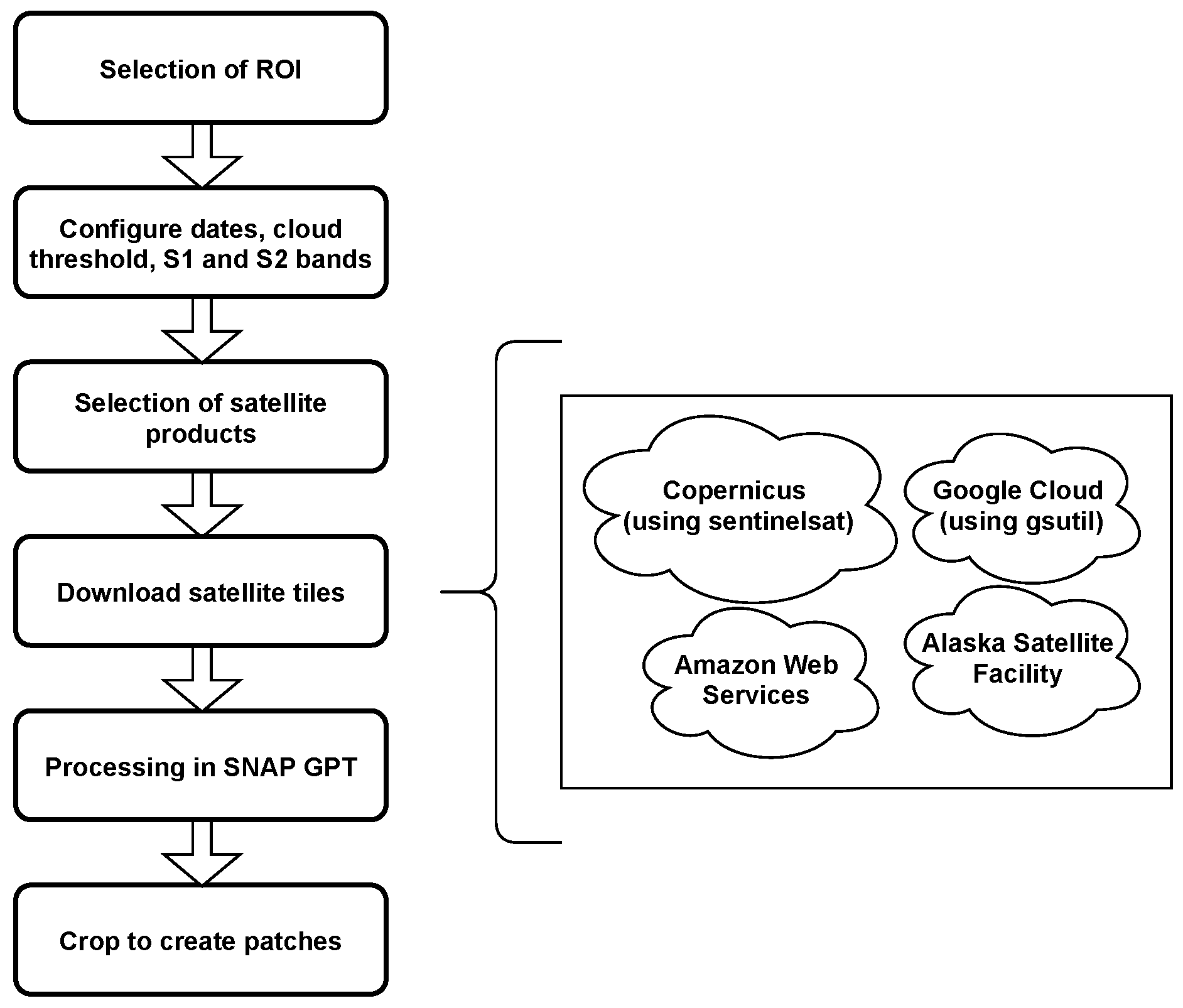
Figure 1. Overview of the proposed ARD framework.
Remotesensing 14 01120 g001
Figure 2. Flow chart for the selection of Sentinel-1 and Sentinel-2 products.
Remotesensing 14 01120 g002
Figure 3. Processing pipeline for Sentinel-1. The suggested framework implements this pipeline using the Graph Processing Tool (GPT) of the ESA SNAP toolbox.
Remotesensing 14 01120 g003
Figure 4. Example of intermediate processing outputs for a Sentinel-1 SAR image (VV polarisation): (a) Subset of the original VV band, (b) Radiometrically calibrated VV band, (c) Speckle filtering output, (d) Terrain-corrected VV band.
Remotesensing 14 01120 g004
Figure 5. SNAP processing pipeline for Sentinel-2.
Remotesensing 14 01120 g005
Figure 6. SNAP processing pipeline for collocated Sentinel-1 and Sentinel-2.
Remotesensing 14 01120 g006
Figure 7. Example of selection of Sentinel-1 and Sentinel-2 products for the ROI shown in violet: (a) Selection of Sentinel-2 product shown in red from all the available overlapping Sentinel-2 products in black, (b) Selection of Sentinel-1 product shown in blue corresponding to the Sentinel-2 product selected in (a) from all the available overlapping Sentinel-1 products in black. The intersection of the ROI and Sentinel-2 is shown in orange. Base layer ©OpenStreetMap contributors in EPSG:32630 UTM projection in Quantum Geographic Information System (QGIS) software.
Remotesensing 14 01120 g007
Figure 8. Example of Sentinel-1 and Sentinel-2 ARD generated with the proposed framework for the ROI selected in Figure 7: (a) ROI division, (b) Sentinel-1 mosaicking shown in false colour composite with red channel as VV, green channel as VH and blue channel as VV/VH, (c) Sentinel-2 RGB mosaicking. Base layer ©OpenStreetMap contributors.
Remotesensing 14 01120 g008
Figure 9. Collocated Sentinel-1 and Sentinel-2 patch: (a) False colour composite of a Sentinel-1 patch (red channel as VV, green channel as VH and blue channel as VV/VH), (b) RGB colour composite of a Sentinel-2 patch.
Remotesensing 14 01120 g009
Figure 10. Sentinel-2 RGB image patch for a group of farms (highlighted in red) in Scotland acquired two days apart: (a) Copernicus cloud percentage for the whole tile (S2A_MSIL2A_20200721T113321_N0214_R080_T30VWH_20200721T141936) is 19.24%, but the ROI is covered with cloud. (b) Copernicus cloud percentage for the whole tile (S2B_MSIL2A_20200723T112119_N0214_R037_T30VWH_20200723T132450) is 90.83%, but the ROI is cloud-free.
Remotesensing 14 01120 g010
Figure 11. Sentinel-1 tile S1A_IW_GRDH_1SDV_20191012T063817_20191012T063842_029422_0358AF _5701 Amplitude VH footprint. The footprint provided by Copernicus is highlighted in red, no-data layer is highlighted in yellow, buffered footprint is highlighted in green.
Remotesensing 14 01120 g011
Figure 12. Regions of interest covering one, two and four Sentinel-2 tiles shown by A, B and C, respectively. The Sentinel-2 tile grid is shown in black, with the tile ID at the centre of each tile. Base layer ©OpenStreetMap contributors.
Remotesensing 14 01120 g012
Figure 13. Example of Sentinel-1 and Sentinel-2 multi-temporal attributes from the 29 May 2020 to the 12 August 2020 for a field growing peas in Scotland. (a) Mean NDVI trend for Sentinel-2 for the cloud-free acquisitions along with examples of RGB images and NDVI maps. (b) Mean of Sentinel-1 VV and VH polarisation normalised radar cross-section (RCS) along with examples of Sentinel-1 false colour composite images.
Remotesensing 14 01120 g013
Table 1. Example of Sentinel-1 and Sentinel-2 product selection showing the overlap with the ROI selected in Figure 7.
ROI SubsetROI Subset
Area (%)
Sentinel Tiles
R160.91Sentinel-1: S1A_IW_GRDH_1SDV_20210421T175920_20210421T175945_037552_046DBA_1823
Sentinel-2: S2B_MSIL2A_20210422T113309_N0300_R080_T30VVH_20210422T130934
R230.79Sentinel-1: S1B_IW_GRDH_1SDV_20210422T175020_20210422T175045_026583_032CA4_6AA2
Sentinel-2: S2B_MSIL2A_20210422T113309_N0300_R080_T30VWH_20210422T130934
R38.29Sentinel-1: S1B_IW_GRDH_1SDV_20210422T175020_20210422T175045_026583_032CA4_6AA2
Sentinel-2: S2B_MSIL2A_20210422T113309_N0300_R080_T30VWJ_20210422T130934
Table 2. Time requirement for the generation of ARD for regions of interest covering one, two and four Sentinel-2 tiles, shown as A, B and C, respectively, in Figure 12.
ScenarioSentinel-2 Tile
Coverage
Selection Time
(s)
Processing
Time (s)
Total Time (s)
A11.2267.8269.0
B22.2343.4345.7
C43.4442.7446.2
Publisher’s Note: MDPI stays neutral with regard to jurisdictional claims in published maps and institutional affiliations.