
Ionospheric Nighttime Enhancements at Low Latitudes Challenge Performance of the Global Ionospheric Maps

 , ,
, ,  ,
, 
Abstract
:1. Introduction
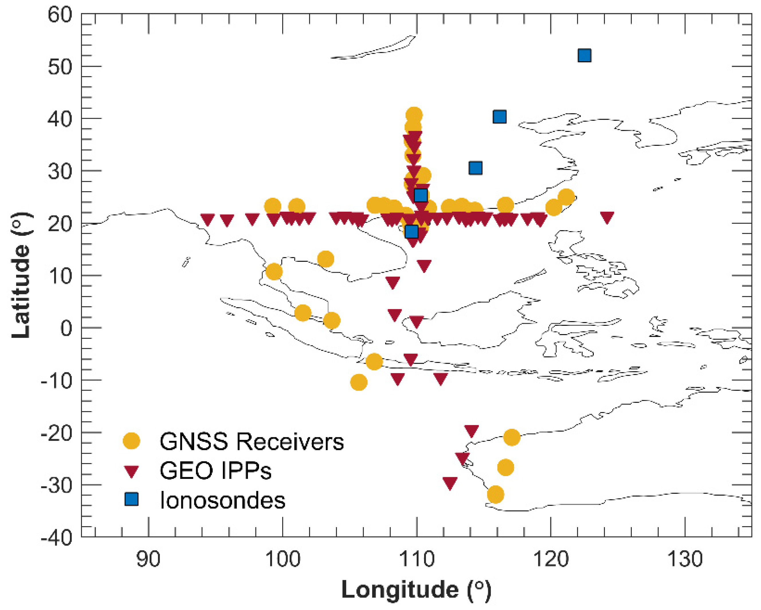
2. Data and Methods
3. Results
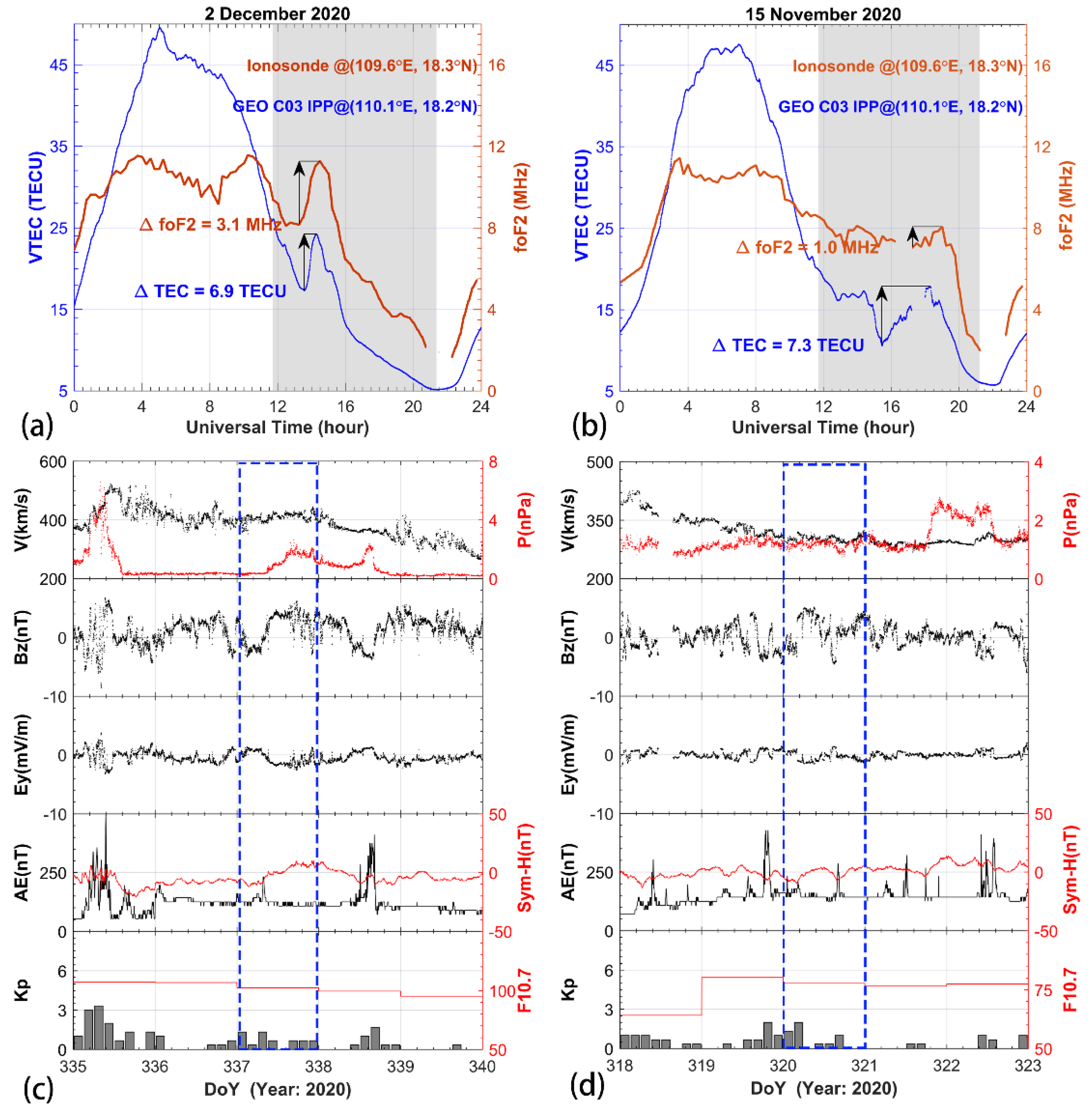
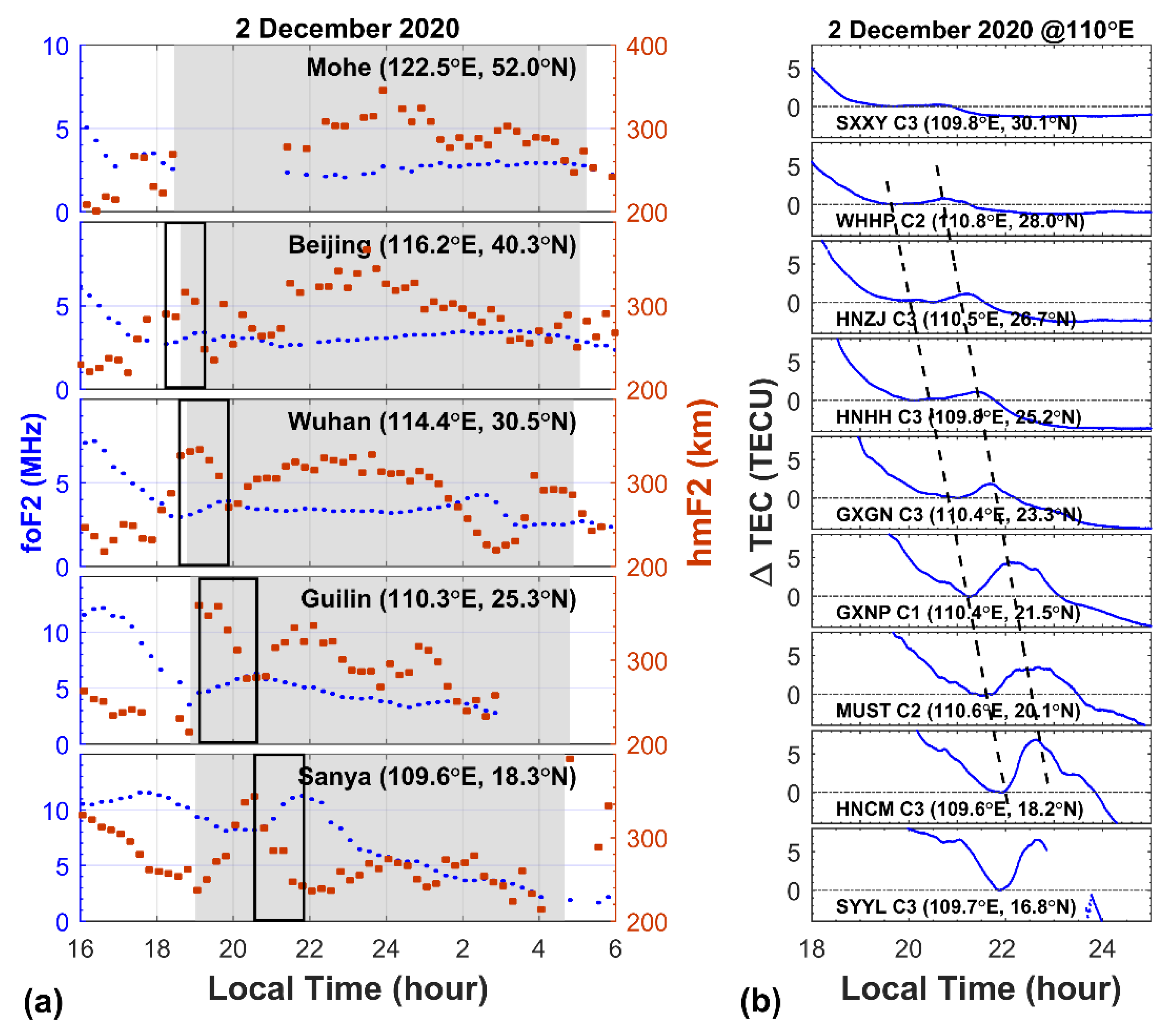
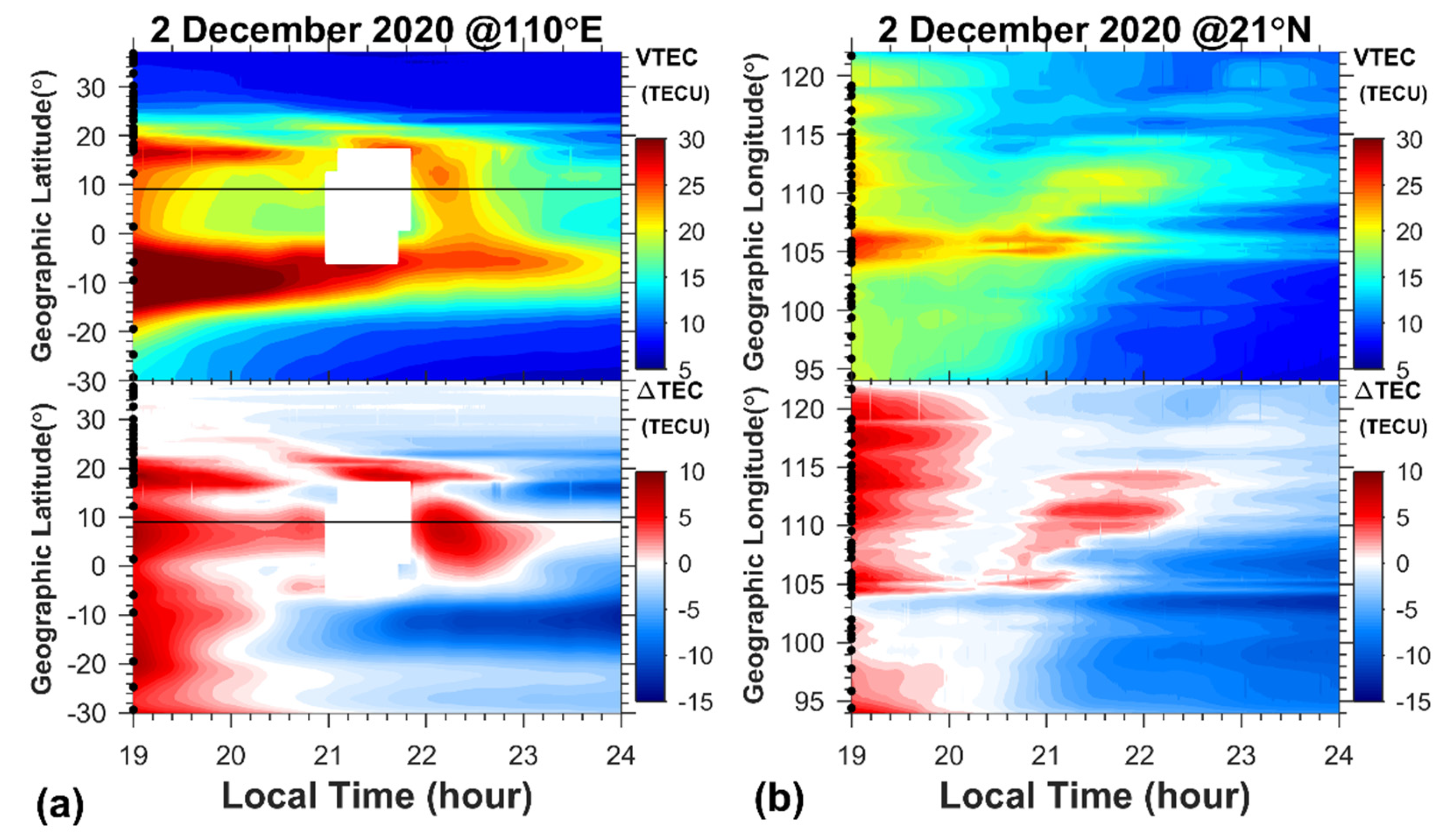
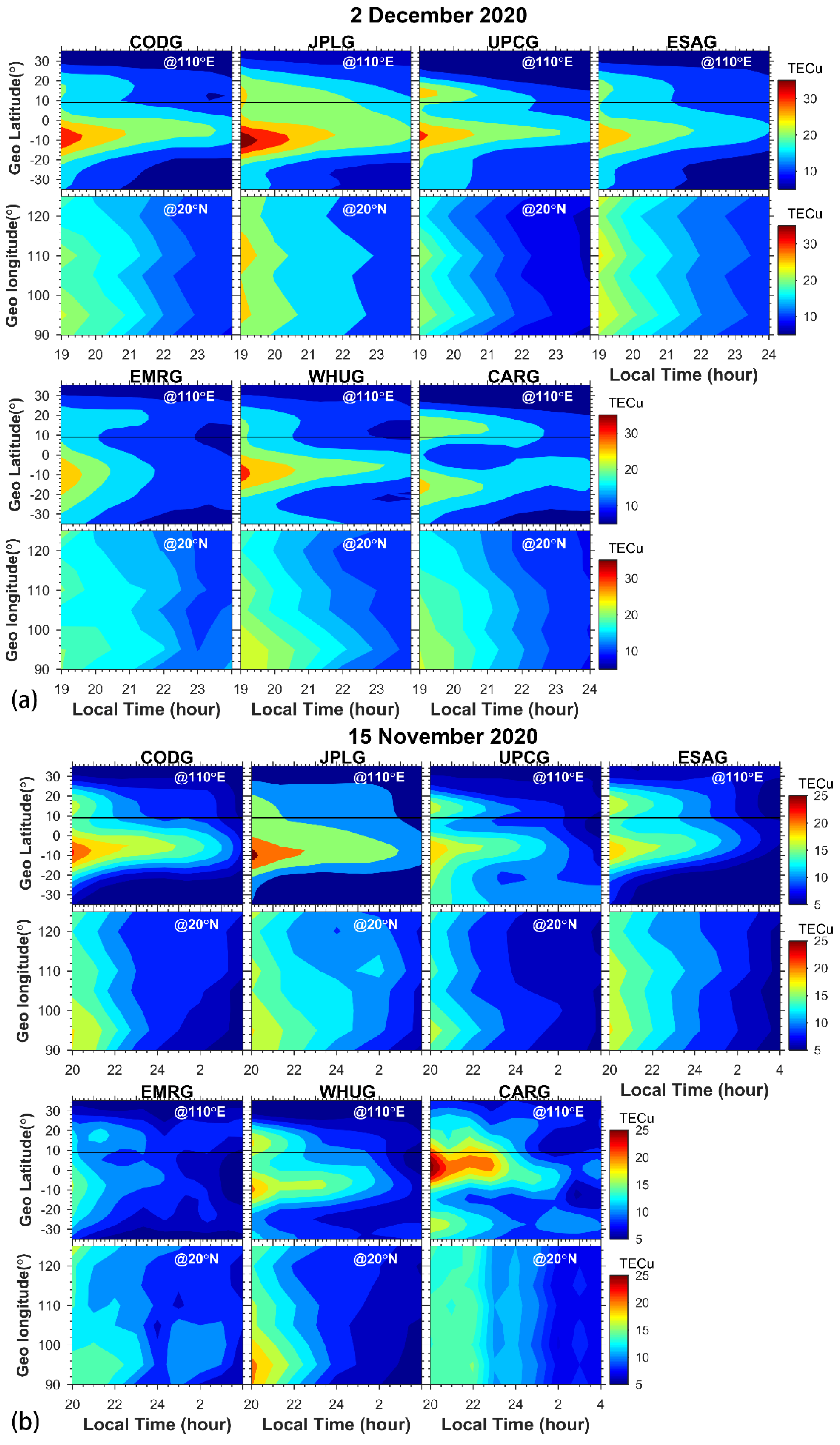
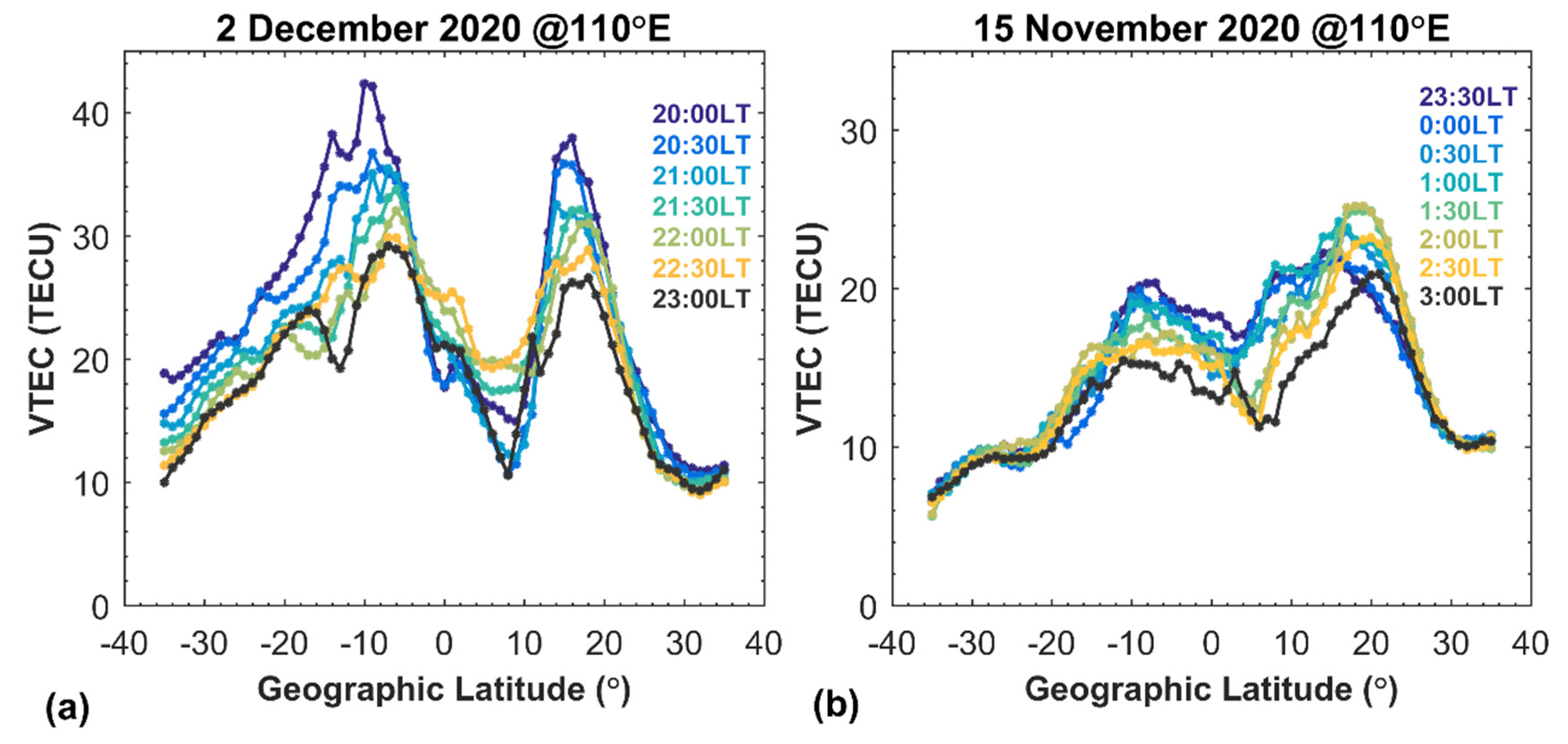
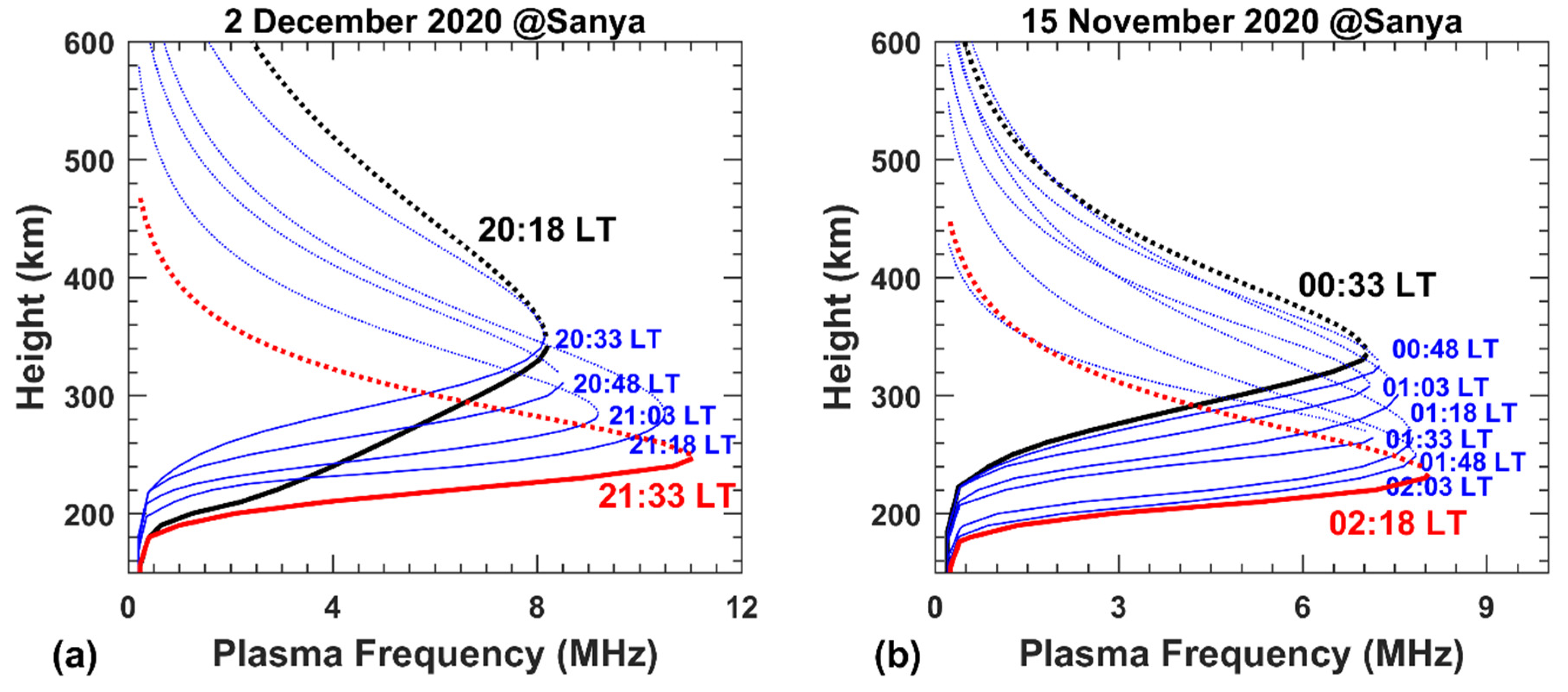
3.1. Case A: 2 December 2020
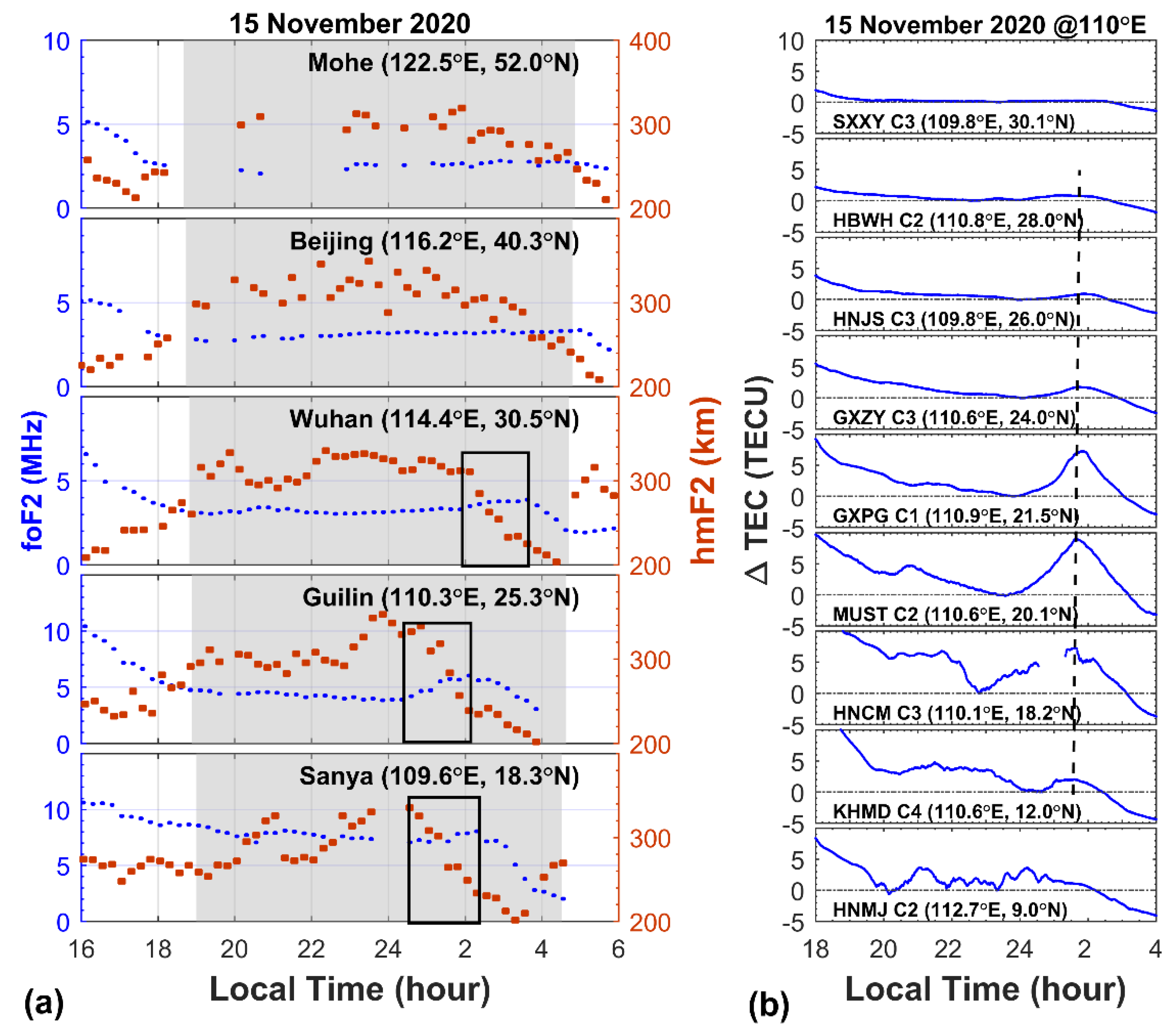
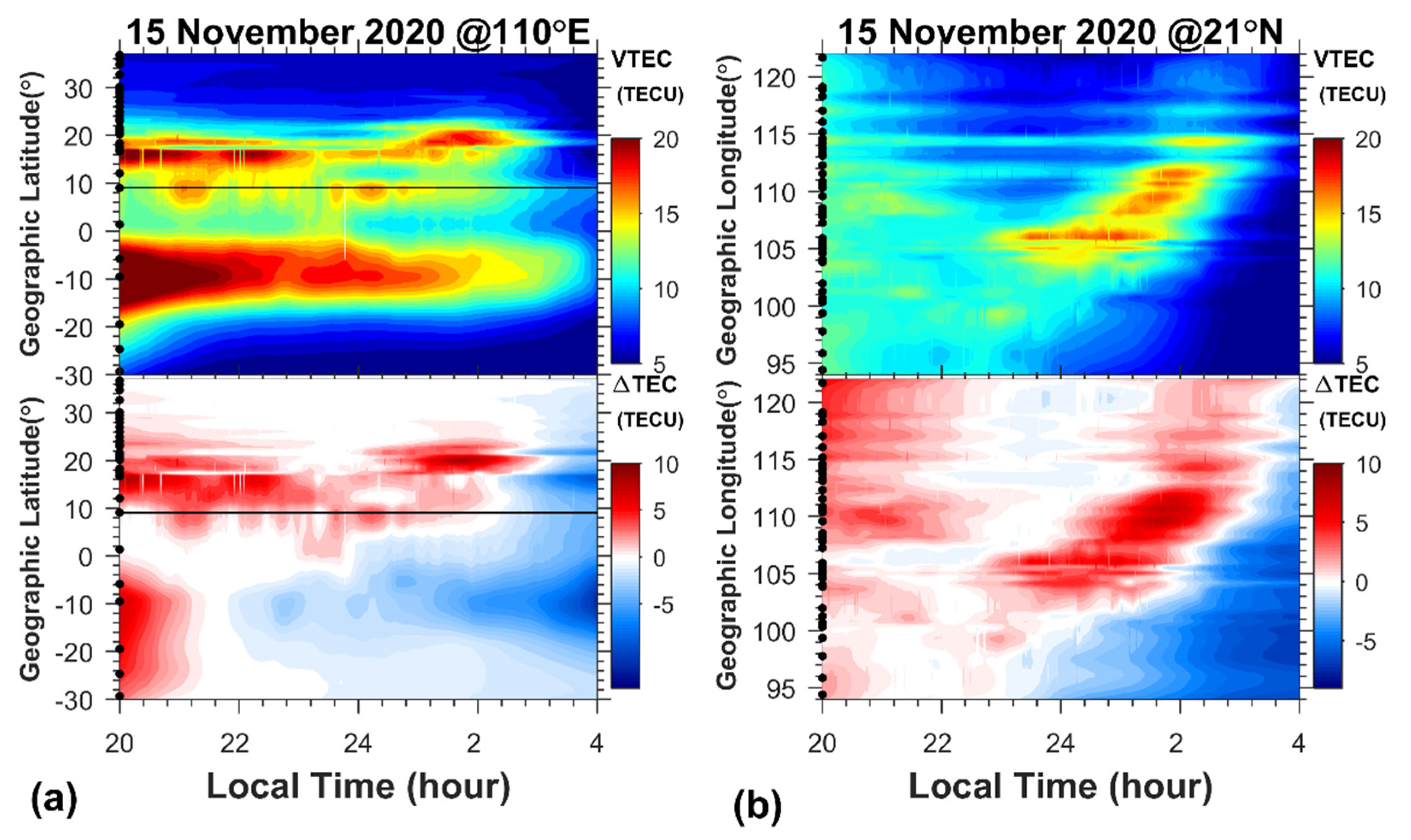
3.2. Case B: 15 November 2020
3.3. Two Cases in GIM
4. Discussion
4.1. Performance of GIMs
4.2. Horizontal and Vertical Variations of INEs
5. Conclusions
Author Contributions
Funding
Data Availability Statement
Acknowledgments
Conflicts of Interest
References
- Mannucci, A.; Wilson, B.; Yuan, D.; Ho, C.; Lindqwister, U.; Runge, T. A global mapping technique for GPS-derived ionospheric total electron content measurements. Radio Sci. 1998, 33, 565–582. [Google Scholar] [CrossRef]
- Hernandez-Pajares, M.; Juan, J.; Sanz, J. New approaches in global ionospheric determination using ground gps data. J. Atmos. Sol. Terr. Phys. 1999, 61, 1237–1247. [Google Scholar] [CrossRef]
- Schaer, S. Mapping and Predicting the Earths Ionosphere Using the Global Positioning System. Ph.D. Dissertation, University of Bern, Bern, Switzerland, 1999. [Google Scholar]
- Wan, W.; Liu, L.; Pi, X.; Zhang, M.-L.; Ning, B.; Xiong, J.; Ding, F. Wavenumber-4 patterns of the total electron content over the low latitude ionosphere. Geophys. Res. Lett. 2008, 35, L12104. [Google Scholar] [CrossRef]
- Mukhtarov, P.; Pancheva, D.; Andonov, B.; Pashova, L. Global TEC maps based on GNSS data: 1. Empirical background TEC model. J. Geophys. Res. Space Phys. 2013, 118, 4594–4608. [Google Scholar] [CrossRef]
- Tariq, M.A.; Shah, M.; Li, Z.; Wang, N.; Shah, M.A.; Iqbal, T.; Liu, L. Lithosphere ionosphere coupling associated with three earthquakes in Pakistan from GPS and GIM TEC. J. Geodyn. 2021, 147, 101860. [Google Scholar] [CrossRef]
- Zhao, J.; Hernández-Pajares, M.; Li, Z.; Wang, N.; Yuan, H. Integrity investigation of global ionospheric TEC maps for high-precision positioning. J. Geod. 2021, 95, 35. [Google Scholar] [CrossRef]
- Jiang, H.; Liu, J.; Wang, Z.; An, J.; Ou, J.; Liu, S.; Wang, N. Assessment of spatial and temporal TEC variations derived from ionospheric models over the polar regions. J. Geod. 2019, 93, 455–471. [Google Scholar] [CrossRef]
- Liu, L.B.; Chen, Y.D.; Zhang, R.L.; Le, H.J.; Zhang, H. Some investigations of ionospheric diurnal variation. Rev. Geophys. Planet. Phys. 2021, 52, 647–661. [Google Scholar] [CrossRef]
- Jee, G.; Lee, H.-B.; Kim, Y.H.; Chung, J.-K.; Cho, J. Assessment of GPS global ionosphere maps (GIM) by comparison between CODE GIM and TOPEX/Jason TEC data: Ionospheric perspective. J. Geophys. Res. Space Phys. 2010, 115, A10319. [Google Scholar] [CrossRef] [Green Version]
- Hernández-Pajares, M.; Roma-Dollase, D.; Krankowski, A.; García-Rigo, A.; Orús-Pérez, R. Methodology and consistency of slant and vertical assessments for ionospheric electron content models. J. Geod. 2017, 91, 1405–1414. [Google Scholar] [CrossRef]
- Li, Z.S.; Wang, N.B.; Li, M.; Zhou, K.; Yuan, Y.B.; Yuan, H. Evaluation and analysis of the global ionospheric TEC map in the frame of international GNSS services. Chin. J. Geophys. 2017, 60, 3718–3729. [Google Scholar] [CrossRef]
- Roma-Dollase, D.; Hernández-Pajares, M.; Krankowski, A.; Kotulak, K.; Ghoddousi-Fard, R.; Yuan, Y.; Li, Z.; Zhang, H.; Shi, C.; Wang, C.; et al. Consistency of seven different GNSS global ionospheric mapping techniques during one solar cycle. J. Geod. 2018, 92, 691–706. [Google Scholar] [CrossRef] [Green Version]
- Klobuchar, J.A. Ionospheric Time-Delay Algorithm for Single-Frequency GPS Users. IEEE Trans. Aerosp. Electron. Syst. 1987, AES-23, 325–331. [Google Scholar] [CrossRef]
- Bellchambers, W.; Piggott, W. Ionospheric Measurements made at Halley Bay. Nature 1958, 182, 1596–1597. [Google Scholar] [CrossRef]
- Evans, J.V. Cause of the mid-latitude evening increase in foF2. J. Geophys. Res. 1965, 70, 1175–1185. [Google Scholar] [CrossRef]
- Essex, E.A.; Klobuchar, J.A. Mid-latitude winter nighttime increases in the total electron content of the ionosphere. J. Geophys. Res. 1980, 85, 6011–6020. [Google Scholar] [CrossRef]
- Balan, N.; Rao, P.B. Latitudinal variations of nighttime enhancements in total electron content. J. Geophys. Res. 1987, 92, 3436–3440. [Google Scholar] [CrossRef]
- Balan, N.; Bailey, G.J. Latitudinal variations of nighttime enhancements in TEC: Solar and magnetic activity effects. Adv. Space Res. 1992, 12, 219–222. [Google Scholar] [CrossRef]
- Balan, N.; Bailey, G.J.; Balachandran Nair, R.; Titheridge, J.E. Nighttime enhancements in ionospheric electron content in the northern and southern hemispheres. J. Atmos. Terr. Phys. 1994, 56, 67–79. [Google Scholar] [CrossRef]
- Mikhailov, A.V.; Leschinkaya, T.Y.; Forster, M. Morphology of NmF2 night-time increases in the Eurasian sector. Ann. Geophys. 2000, 18, 618–628. [Google Scholar] [CrossRef]
- Zhao, B.; Wan, W.; Liu, L.; Igarashi, K.; Nakamura, M.; Paxton, L.J.; Su, S.-Y.; Li, G.; Ren, Z. Anomalous enhancement of ionospheric electron content in the Asian-Australian region during a geomagnetically quiet day. J. Geophys. Res. 2008, 113, A11302. [Google Scholar] [CrossRef] [Green Version]
- He, M.; Liu, L.; Wan, W.; Ning, B.; Zhao, B.; Wen, J.; Yue, X.; Le, H. A study of the Weddell Sea Anomaly observed by FORMOSAT-3/COSMIC. J. Geophys. Res. 2009, 114, A12309. [Google Scholar] [CrossRef] [Green Version]
- Thampi, S.V.; Balan, N.; Lin, C.; Liu, H.; Yamamoto, M. Mid-latitude Summer Nighttime Anomaly (MSNA)—Observations and model simulations. Ann. Geophys. 2011, 29, 157–165. [Google Scholar] [CrossRef] [Green Version]
- Ren, Z.; Wan, W.; Liu, L.; Le, H.; He, M. Simulated midlatitude summer nighttime anomaly in realistic geomagnetic fields. J. Geophys. Res. 2012, 117, A03323. [Google Scholar] [CrossRef] [Green Version]
- Trivedi, R.; Jain, S.; Jain, A.; Gwal, A.K. Solar and magnetic control on night-time enhancement in TEC near the crest of the Equatorial Ionization Anomaly. Adv. Space Res. 2013, 51, 61–68. [Google Scholar] [CrossRef]
- Farelo, A.F.; Herraiz, M.; Mikhailov, A.V. Global morphology of night-time NmF2 enhancements. Ann. Geophys. 2002, 20, 1795–1806. [Google Scholar] [CrossRef] [Green Version]
- Su, Y.Z.; Bailey, G.J.; Balan, N. Night-time enhancements in TEC at equatorial anomaly latitudes. J. Atmos. Sol. Terr. Phys. 1994, 56, 1619–1628. [Google Scholar] [CrossRef]
- Pavlov, A.V.; Pavlova, N.M. Anomalous night-time peaks in diurnal variations of NmF2 close to the geomagnetic equator: A statistical study. J. Atmos. Sol. Terr. Phys. 2007, 69, 1871–1883. [Google Scholar] [CrossRef]
- Luan, X.; Wang, W.; Burns, A.; Solomon, S.C.; Lei, J. Midlatitude nighttime enhancement in F region electron density from global COSMIC measurements under solar minimum winter condition. J. Geophys. Res. 2008, 113, A09319. [Google Scholar] [CrossRef]
- Chen, Y.; Liu, L.; Le, H.; Wan, W.; Zhang, H. NmF2 enhancement during ionospheric F2 region nighttime: A statistical analysis based on COSMIC observations during the 2007–2009 solar minimum. J. Geophys. Res. Space Phys. 2015, 120, 10083–10095. [Google Scholar] [CrossRef]
- Chen, Y.; Liu, L.; Le, H.; Wan, W.; Zhang, H. The global distribution of the dusk-to-nighttime enhancement of summer NmF2 at solar minimum. J. Geophys. Res. Space Phys. 2016, 121, 7914–7922. [Google Scholar] [CrossRef]
- Jiang, C.; Deng, C.; Yang, G.; Liu, J.; Zhu, P.; Yokoyama, T.; Song, H.; Lan, T.; Zhou, C.; Wu, X.; et al. Latitudinal variation of the specific local time of postmidnight enhancement peaks in F layer electron density at low latitudes: A case study. J. Geophys. Res. Space Phys. 2016, 121, 3476–3483. [Google Scholar] [CrossRef] [Green Version]
- Li, Z.; Wang, N.; Liu, A.; Yuan, Y.; Wang, L.; Hernández-Pajares, M.; Krankowski, A.; Yuan, H. Status of CAS global ionospheric maps after the maximum of solar cycle 24. Satell. Navig. 2021, 2, 19. [Google Scholar] [CrossRef]
- Ho, C.M.; Mannucci, A.J.; Lindqwister, U.J.; Pi, X.; Tsurutani, B.T. Global ionosphere perturbations monitored by the worldwide GPS network. Geophys. Res. Lett. 1996, 23, 3219–3222. [Google Scholar] [CrossRef] [Green Version]
- Hernández-Pajares, M.; Juan, J.M.; Sanz, J. Neural network modeling of the ionospheric electron content at global scale using GPS data. Radio Sci. 1997, 32, 1081–1089. [Google Scholar] [CrossRef] [Green Version]
- Komjathy, A.; Sparks, L.; Wilson, B.D.; Mannucci, A.J. Automated daily processing of more than 1000 ground-based GPS receivers for studying intense ionospheric storms. Radio Sci. 2005, 40, RS6006. [Google Scholar] [CrossRef] [Green Version]
- Orús, R.; Hernández-Pajares, M.; Juan, J.M.; Sanz, J. Improvement of global ionospheric VTEC maps by using kriging interpolation technique. J. Atmos. Sol.-Terr. Phys. 2005, 67, 1598–1609. [Google Scholar] [CrossRef]
- Feltens, J. Development of a new three-dimensional mathematical ionosphere model at European Space Agency/European Space Operations Centre. Space Weather 2007, 5, S12002. [Google Scholar] [CrossRef] [Green Version]
- Zhang, H.; Xu, P.; Han, W.; Ge, M.; Shi, C. Eliminating negative VTEC in global ionosphere maps using inequality-constrained least squares. Adv. Space Res. 2013, 51, 988–1000. [Google Scholar] [CrossRef]
- Li, Z.; Yuan, Y.; Wang, N.; Hernandez-Pajares, M.; Huo, X. SHPTS: Towards a new method for generating precise global ionospheric TEC map based on spherical harmonic and generalized trigonometric series functions. J. Geod. 2015, 89, 331–345. [Google Scholar] [CrossRef]
- Huang, X.; Reinisch, B.W. Vertical electron content from ionograms in real time. Radio Sci. 2001, 36, 335–342. [Google Scholar] [CrossRef] [Green Version]
- Hu, L.; Yue, X.; Ning, B. Development of the Beidou Ionospheric Observation Network in China for space weather monitoring. Space Weather 2017, 15, 974–984. [Google Scholar] [CrossRef]
- Wang, C. New Chains of Space Weather Monitoring Stations in China. Space Weather 2010, 8, S08001. [Google Scholar] [CrossRef]
- Beutler, G.; Rothacher, M.; Schaer, S.; Springer, T.A.; Kouba, J.; Neilan, R.E. The International GPS Service (IGS): An interdisciplinary service in support of Earth sciences. Adv. Space Res. 1999, 23, 631–653. [Google Scholar] [CrossRef]
- Liu, L.; Chen, Y.; Le, H.; Ning, B.; Wan, W.; Liu, J.; Hu, L. A case study of postmidnight enhancement in F-layer electron density over Sanya of China. J. Geophys. Res. Space Phys. 2013, 118, 4640–4648. [Google Scholar] [CrossRef]
- Chen, Y.; Ma, G.; Huang, W.; Shen, H.; Li, J. Night-time total electron content enhancements at equatorial anomaly region in China. Adv. Space Res. 2008, 41, 617–623. [Google Scholar] [CrossRef]
Publisher’s Note: MDPI stays neutral with regard to jurisdictional claims in published maps and institutional affiliations. |
© 2022 by the authors. Licensee MDPI, Basel, Switzerland. This article is an open access article distributed under the terms and conditions of the Creative Commons Attribution (CC BY) license (https://creativecommons.org/licenses/by/4.0/).
Share and Cite
Yang, Y.; Liu, L.; Zhao, X.; Xie, H.; Chen, Y.; Le, H.; Zhang, R.; Tariq, M.A.; Li, W. Ionospheric Nighttime Enhancements at Low Latitudes Challenge Performance of the Global Ionospheric Maps. Remote Sens. 2022, 14, 1088. https://doi.org/10.3390/rs14051088
Yang Y, Liu L, Zhao X, Xie H, Chen Y, Le H, Zhang R, Tariq MA, Li W. Ionospheric Nighttime Enhancements at Low Latitudes Challenge Performance of the Global Ionospheric Maps. Remote Sensing. 2022; 14(5):1088. https://doi.org/10.3390/rs14051088
Chicago/Turabian StyleYang, Yuyan, Libo Liu, Xiukuan Zhao, Haiyong Xie, Yiding Chen, Huijun Le, Ruilong Zhang, M. Arslan Tariq, and Wenbo Li. 2022. "Ionospheric Nighttime Enhancements at Low Latitudes Challenge Performance of the Global Ionospheric Maps" Remote Sensing 14, no. 5: 1088. https://doi.org/10.3390/rs14051088
APA StyleYang, Y., Liu, L., Zhao, X., Xie, H., Chen, Y., Le, H., Zhang, R., Tariq, M. A., & Li, W. (2022). Ionospheric Nighttime Enhancements at Low Latitudes Challenge Performance of the Global Ionospheric Maps. Remote Sensing, 14(5), 1088. https://doi.org/10.3390/rs14051088