Article

Using Ensemble-Based Systems with Near-Infrared Hyperspectral Data to Estimate Seasonal Snowpack Density

INRS-Institut National de la Recherche Scientifique (INRS), Québec, QC G1K 9A9, Canada
*
Author to whom correspondence should be addressed.
Remote Sens. 2022, 14(5), 1089; https://doi.org/10.3390/rs14051089
Submission received: 31 December 2021 / Revised: 3 February 2022 / Accepted: 21 February 2022 / Published: 23 February 2022
(This article belongs to the Special Issue Hyperspectral Remote Sensing: Current Situation and New Challenges)

Abstract

:
Estimating the seasonal density of the snowpack has many financial and environmental benefits. Rapid assessment and daily monitoring of its evolution are therefore key to effective prevention. Traditionally, the physical characteristics of snow are measured directly in the field, which involves high costs and personnel mobilization. Hyperspectral imaging is a reliable and efficient technique to study and evaluate this physical property. The spectral reflectance of snow is partly defined by changes in its physical properties, particularly in the Near infrared (NIR) part of the spectrum. Recently, a hybrid snow density estimation model allowing retrieval of density from NIR hyperspectral data was developed, based on an a priori classification of snow samples. However, in order to obtain optimal density estimates with the Hybrid model (HM), the sources of classification and estimation error must be controlled. Following the same principle as the HM, an Ensemble-based system (EBS) was developed. This model reduces the number of misclassification errors produced by the HM. The general concept of EBS algorithms is based on the principle that obtaining more opinions before making a decision is part of human nature, especially when economic and environmental benefits are at stake. This approach has helped to reduce the risk of classification and estimation errors and to develop more robust density results. One hundred and fourteen snow samples collected during three winters (2018–2020) were used to calibrate and validate the EBS. The performance of the EBS was validated using an independent database and the results were satisfactory (R2 = 0.90, RMSE = 44.45 kg m−3, BIAS = 3.87 kg m−3 and NASH = 0.89).

1. Introduction

The measurement and modelling of the physical characteristics of snow, particularly its density, is important for financial and environmental purposes, as this property is essential when estimating the water equivalent of snow, predicting avalanche risk [1] and it is often used to observe and understand the evolution of seasonal snowpacks [2,3]. The physical characteristics of natural snow can vary vertically and horizontally in the snowpack [4,5]. Daily monitoring and advances in measurement techniques for these features are key elements in controlling and reducing the risks related to measurement uncertainties [6], but they requires a significant effort in measuring and collecting samples in the field to ensure the accuracy of the measurements. It has also been shown that standard sampling methods, based on fixed sampling points, insufficiently cover large areas and the resulting temporal resolution is deficient [6,7,8]. High resolution measurement techniques based on remote sensing can be used to validate and improve current physical measurement operations.
Due to its ability to provide information over a wide range of wavelengths, Near infrared (NIR) hyperspectral technology is a promising tool to estimate the physical properties of snow [9,10]. This innovative technique provides useful information on the physical and chemical components of a scanned sample [11,12,13], which can be used for modelling purposes. Indeed, the NIR spectral range has been tested in the laboratory and in the field in several works aimed at estimating the physical properties of snow [4,14,15,16,17]. This is made possible by relating the observed optical changes in the NIR spectral reflectance at specific wavelengths to the physical transformation processes of snow [9,16,18,19]. A review of scientific literature has shown that few works have been dedicated to estimating snow density from optical data. Nonetheless, Gergely, et al. [18] demonstrated that snow density values can be estimated in a cold laboratory using NIR transmittance measurements if the size and shape of the snow grains are known in advance. Varade [10] developed a new approach to estimate snow moisture and density using the infrared bands available with most spectral sensors. Their method based on using the NIR band led them to develop the Normalized difference snow index (NDSI), called PIR-NDSI space.
Recently, a Hybrid model (HM) based on NIR spectral data was developed to estimate snow density [19]. Density estimation using the HM is carried out in two steps: (1) The snow samples are classified into one of three snow classes (Weakly to moderately metamorphosed (WMM), Moderately to highly metamorphosed (MHM) and Highly to very highly metamorphosed (HVM)) and (2) specific estimators corresponding to the selected snow classes are used to estimate the density. When using this model, the selection of the final estimator is critical because the selection of a wrong estimator could lead to the over- or underestimation of density. Moreover, classification algorithms, such as the one used to develop the HM (classification and regression tree), are known to be local and unstable [20]. This instability significantly affects model reliability when used to estimate the density of snow.
In such complex modelling contexts, many authors suggest that the use of an Ensemble-based system (EBS) could lead to more stable and robust results [21,22,23,24,25,26,27]. Two conditions are necessary to build a stable and robust EBS: (1) reaching a high diversity between individual elements (either classifiers, estimators, or both) and (2) applying effective rules to combine individual elements in a way that good decisions are amplified and bad decisions are cancelled [28].
To achieve the desired diversity, EBSs are composed of thousands of different elements, which can be problematic when using remote sensing data. Researchers are often faced with a delicate situation: either reduce the number of features in the EBS which could reduce the solution space or develop a robust EBS with a very long running time. The Gaussian quadrature formula (GQF) could provide an interesting solution to this problem. This method, which is frequently used in uncertainty propagation analysis [29], transforms the problem of a sample with a very large number of solutions (which require laborious integral calculations) into a weighted sum of optimal solutions through simple and accurate numerical solution techniques [30].
The objective of our work is to develop an EBS on the foundation of the previously described HM and GQF to estimate the seasonal density of the snowpack using high-resolution NIR hyperspectral data. The EBS was evaluated by independent validation data and its performance was assessed using four statistical evaluation indices (R2, Root mean square error (RMSE), BIAS, and Nash-criterion (NASH)).

2. Materials and Methods

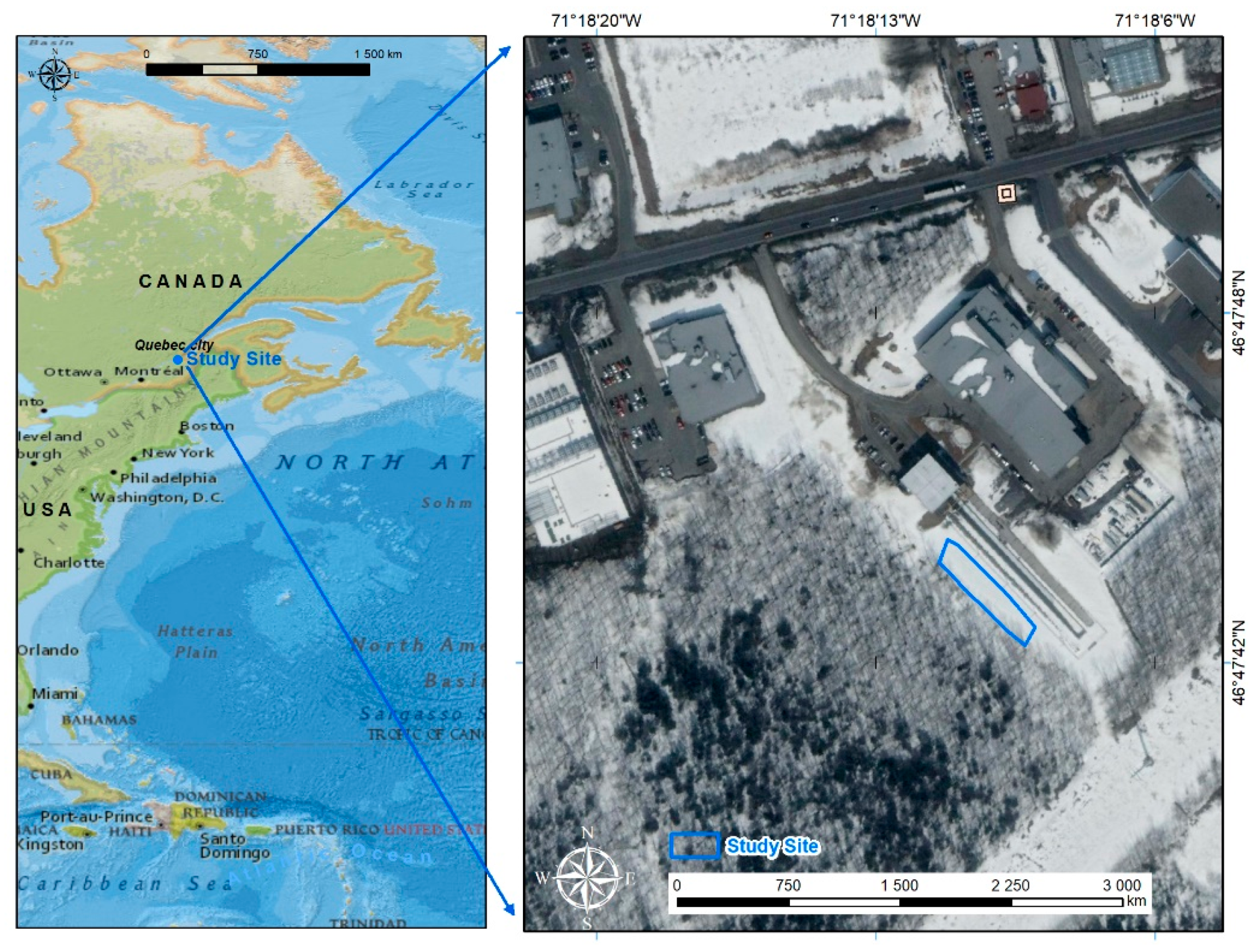
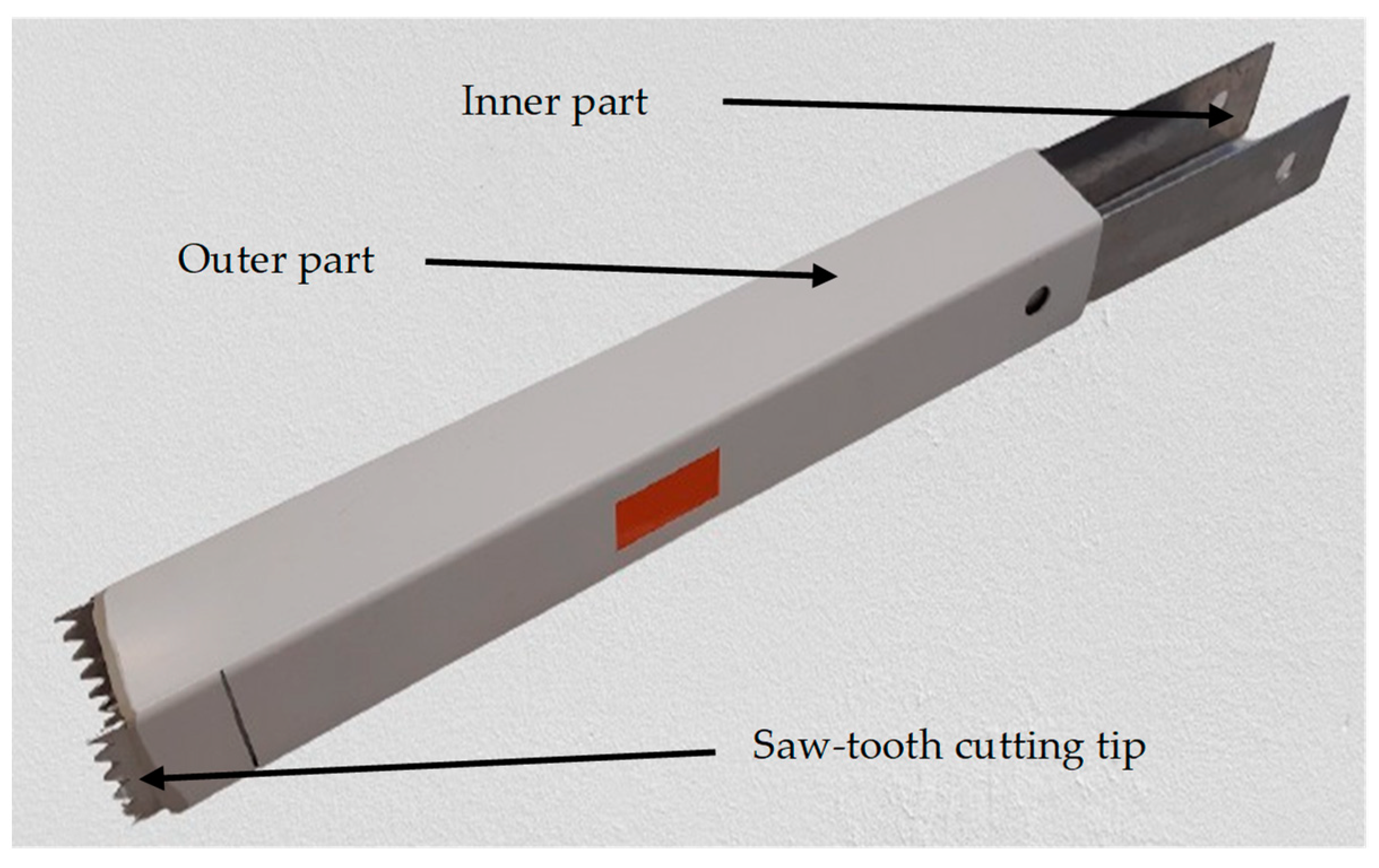
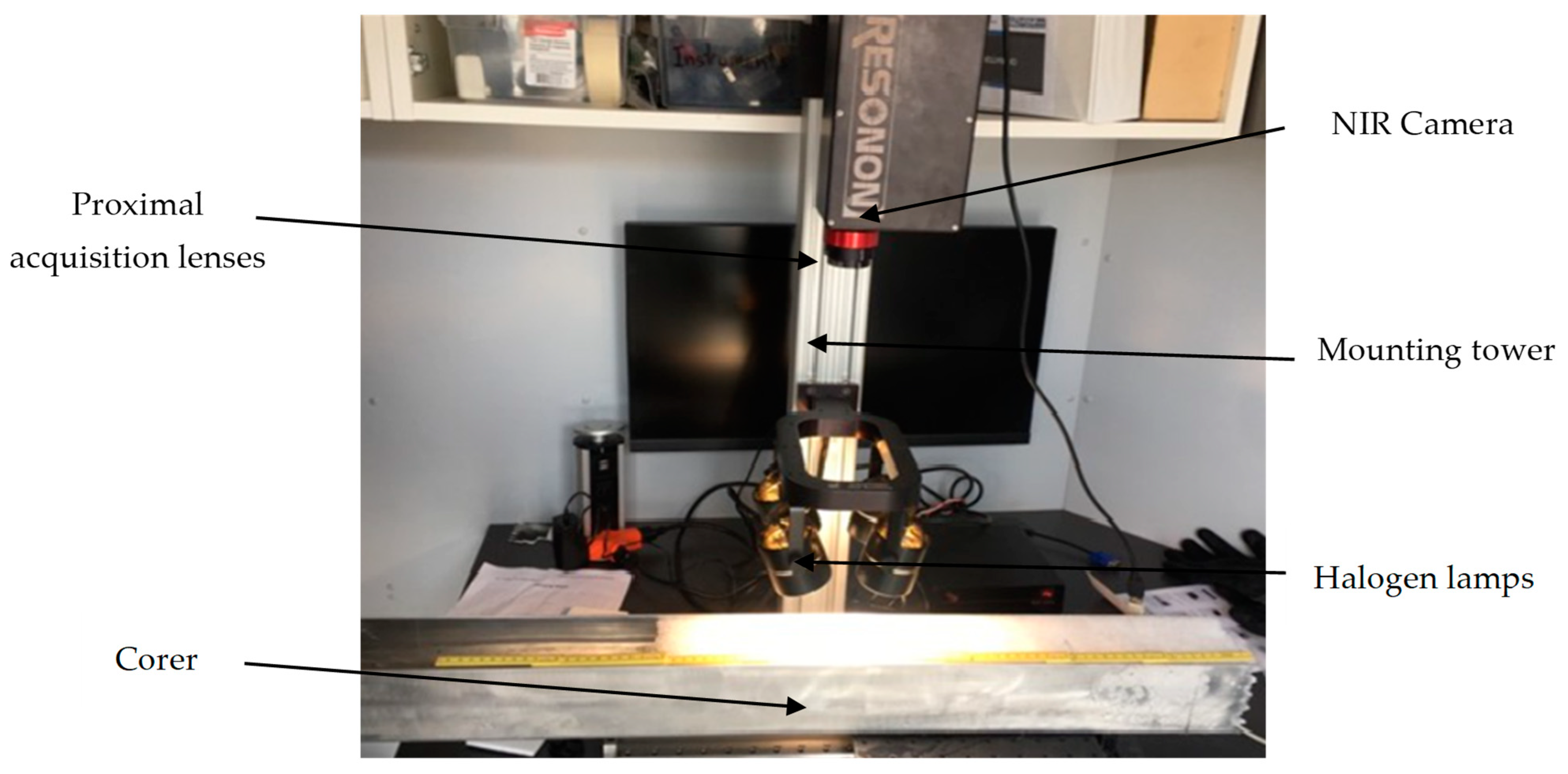
2.1. In Situ Measurements for the Calibration and Validation Database

To achieve the objectives of this study, the calibration and validation databases were composed of two types of data: optical data (spectral reflectance) measured with a proximal acquisition station, and physical data (grain size, grain type, and density) sampled with a snow corer. For all acquisitions, the same equipment and sampling technique was used throughout the study. The study site was located at the INRS’s (National Institute of Scientific Research) Technology Park in the City of Quebec (46°47′43.22′′N and −71°18′10′′W; Figure 1). The area selected for this study is approximately 20 m2, located in an open sector of the experimental site.
The portable rectangular snow corer was designed and built by the INRS’s remote sensing team and is shown in Figure 2. It is used to recover the vertical stratigraphy of the snowpack which allows measuring of the physical and optical properties of the recovered profile. The dimensions of the corer make it possible to recover the entire vertical profile of the snowpack because of its simple operating principle. The corer is made up of two parts, the inner part is made of metal and the outer part of plastic, with a triangular saw-tooth cutting tip. The device is simply inserted into the snow at the required depth. A trench is then made to access the lower part of the corer and a plate is placed under to prevent the snow from falling. The corer is then tilted horizontally and transported to the measurement station. At this point, the handle is pulled and the inner part containing the snow is carefully removed. The snow is only minimally disturbed during the sampling process, resulting in accurate measurements.
The proximal acquisition station used in this work consists of a RESONON PIKA NIR line-scanning hyperspectral camera that allows for the measurement of NIR spectral reflectance at several wavelengths between 900 and 1700 nm, with a spectral resolution of 5.5 nm and 148 spectral bands. The reflectance was calculated by measuring the radiance reflected from the snow surface and from a reference target. The latter has near-Lambertian reflection properties when viewed from the nadir. The station is also equipped with a halogen lighting system, mounting tower, linear translation stage for rapid image acquisition, data acquisition software (Spectronon Pro (Resonon Inc., Bozeman, MT, USA)) and proximal acquisition lenses, as shown in Figure 3.
Once the snow profile has been recovered, the core drill is then placed horizontally on the moving platform in relation to the camera’s field of view (nadir) to record a high spectral resolution image, which is then analyzed with Spectronon Pro software. This image is used to validate the identification of snow layers already measured in the field and to analyze the spectral response of each identified layer. The speed of the platform was selected to achieve equal spatial resolution of the vertical and horizontal axes to avoid distortion of the image size and to fit the predetermined exposure time of the camera.
In situ sampling of the physical properties of snow is carried out by treating the recovered snow profile as a succession of layers. Each visually homogeneous layer is carefully removed from the sampler and the size and type of snow grains are measured using a millimeter grid and a 10× magnifying glass. The sample is then classified according to the International Classification of Seasonal Snow on the Ground [31]. Finally, the isolated layer was weighed to determine its density based on its mass and volume. To ensure consistency in the analysis, all observations and measurements were made by the same person.

2.2. Algorithm Development

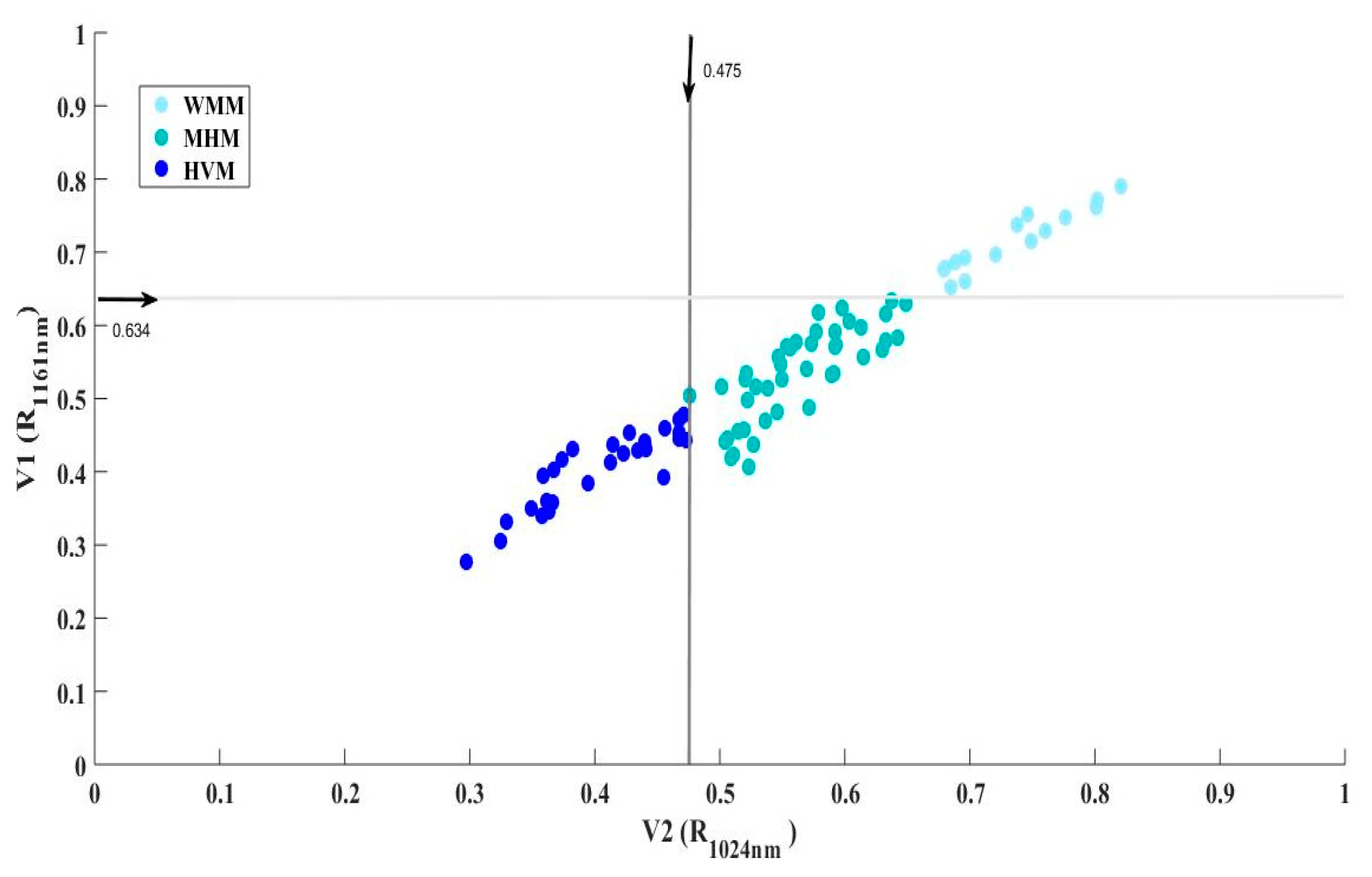
2.2.1. The Hybrid Model

The HM developed by El Oufir, [19] to estimate seasonal snowpack density from hyperspectral data is composed of a classifier and three estimators, each specific to a given snow class (WMM, MHM, and HVM). The HM classifier was trained using the Classification and regression tree (CART) method [32]. Once trained, it was possible to divide the calibration database into the three specific classes mentioned above, based on the reflectance value of the samples at wavelengths 1024 nm and 1161 nm [19]. The classifier was then used to calibrate the three specific estimators of the HM (Figure 4) using a stepwise multivariate regression. Density estimation using the HM is performed in two steps:
Classification of the snow samples into one of the three snow classes using the classifier of the HM;
Estimation of each class’s density using the corresponding specific estimator [19].

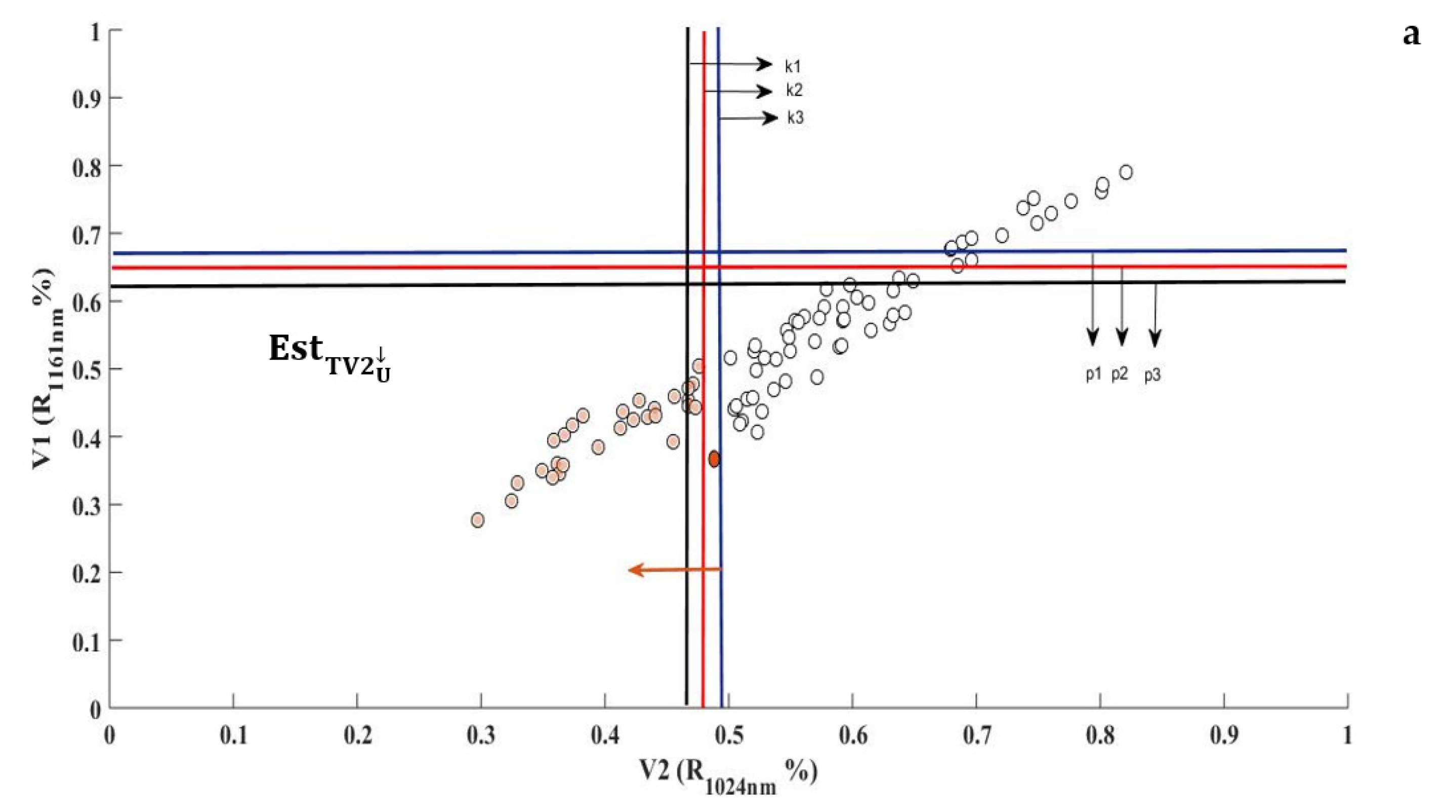
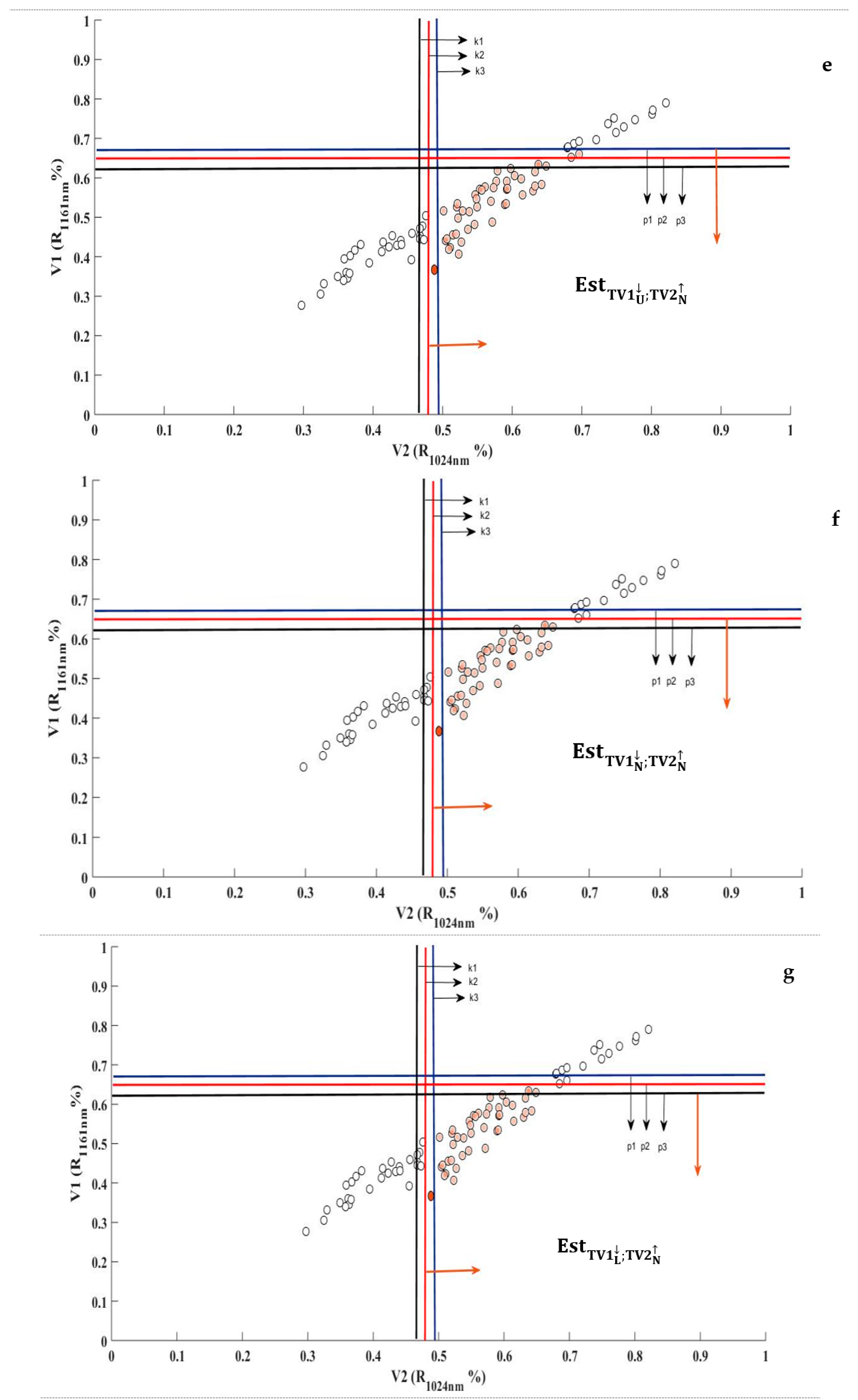
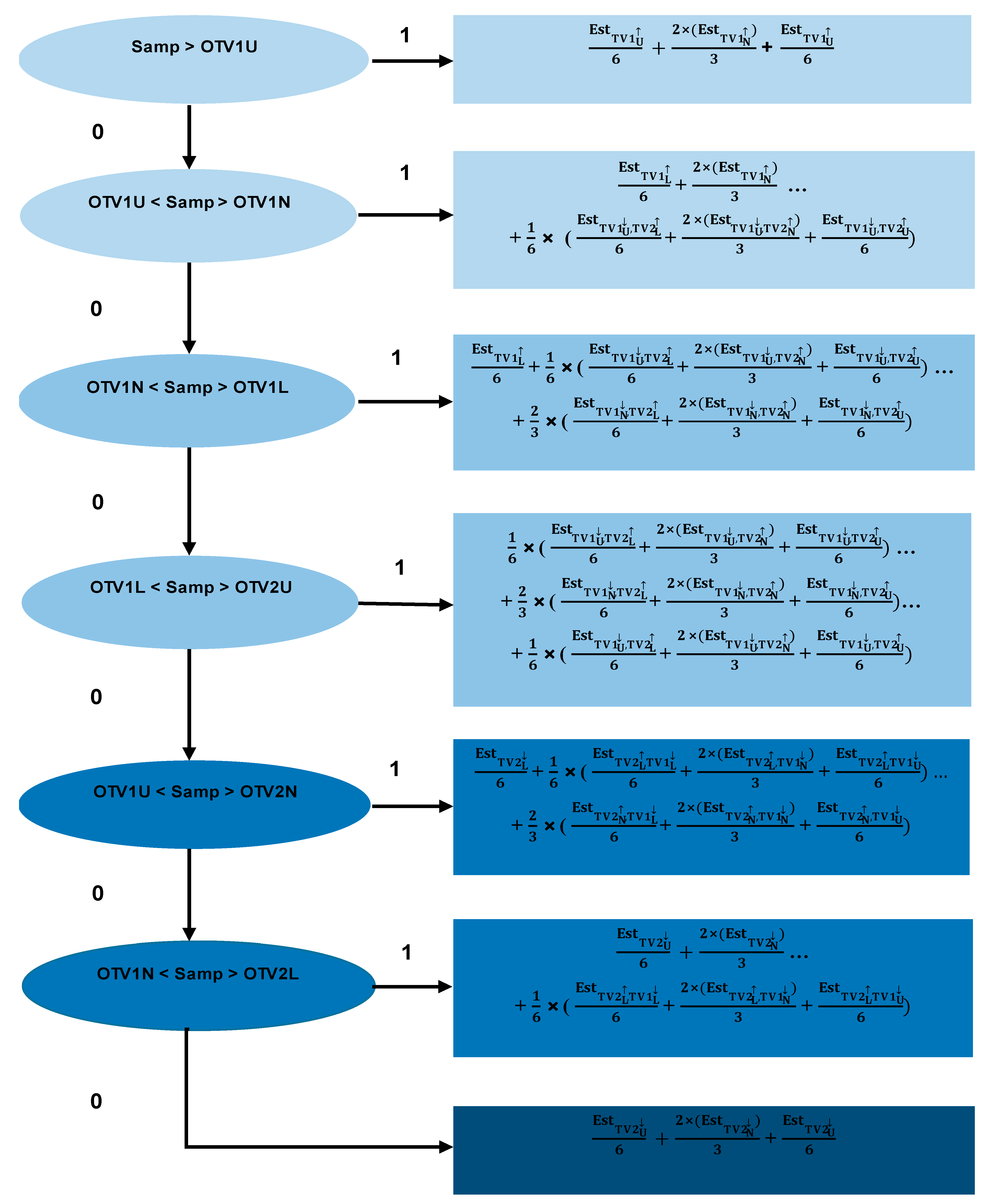
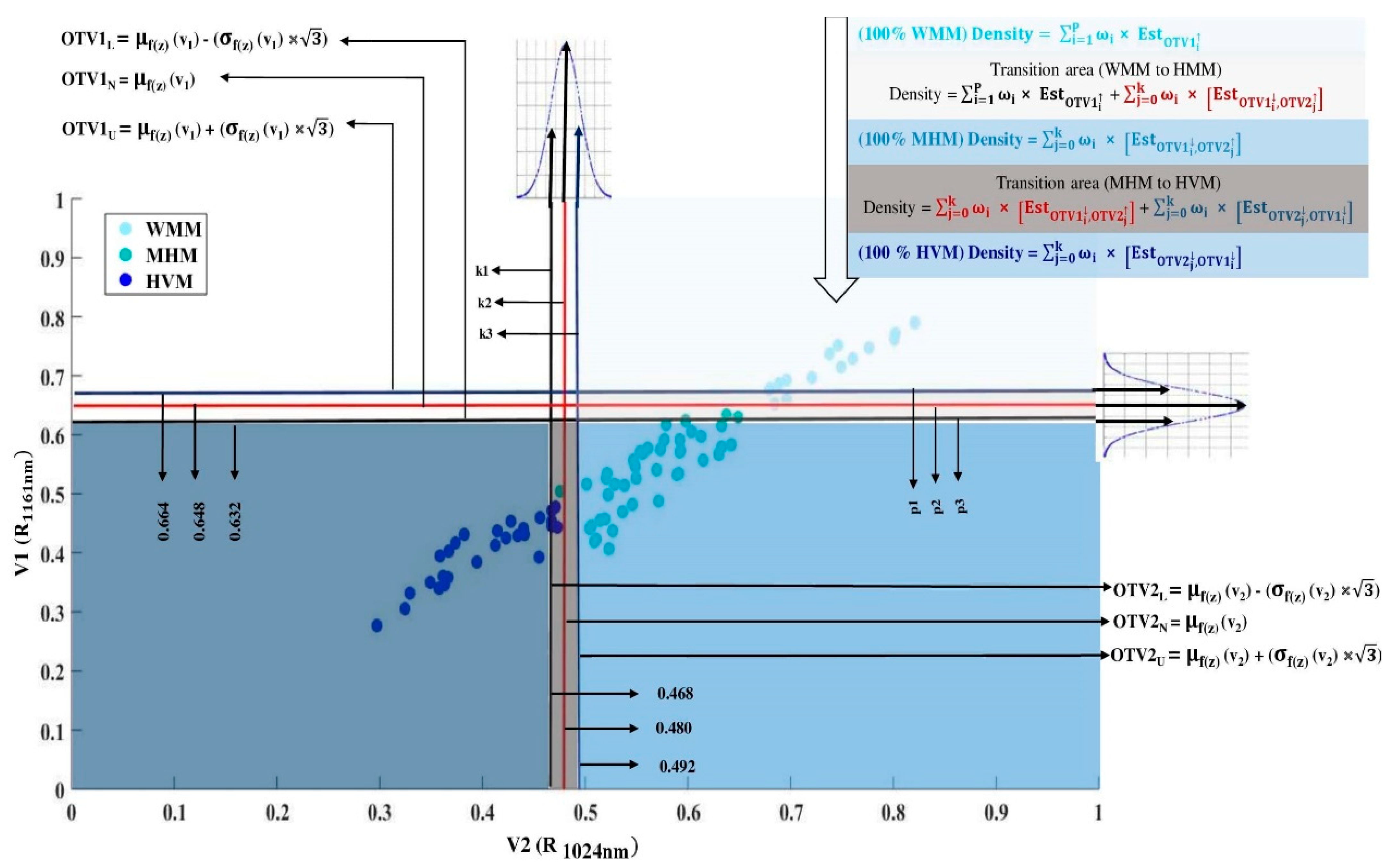
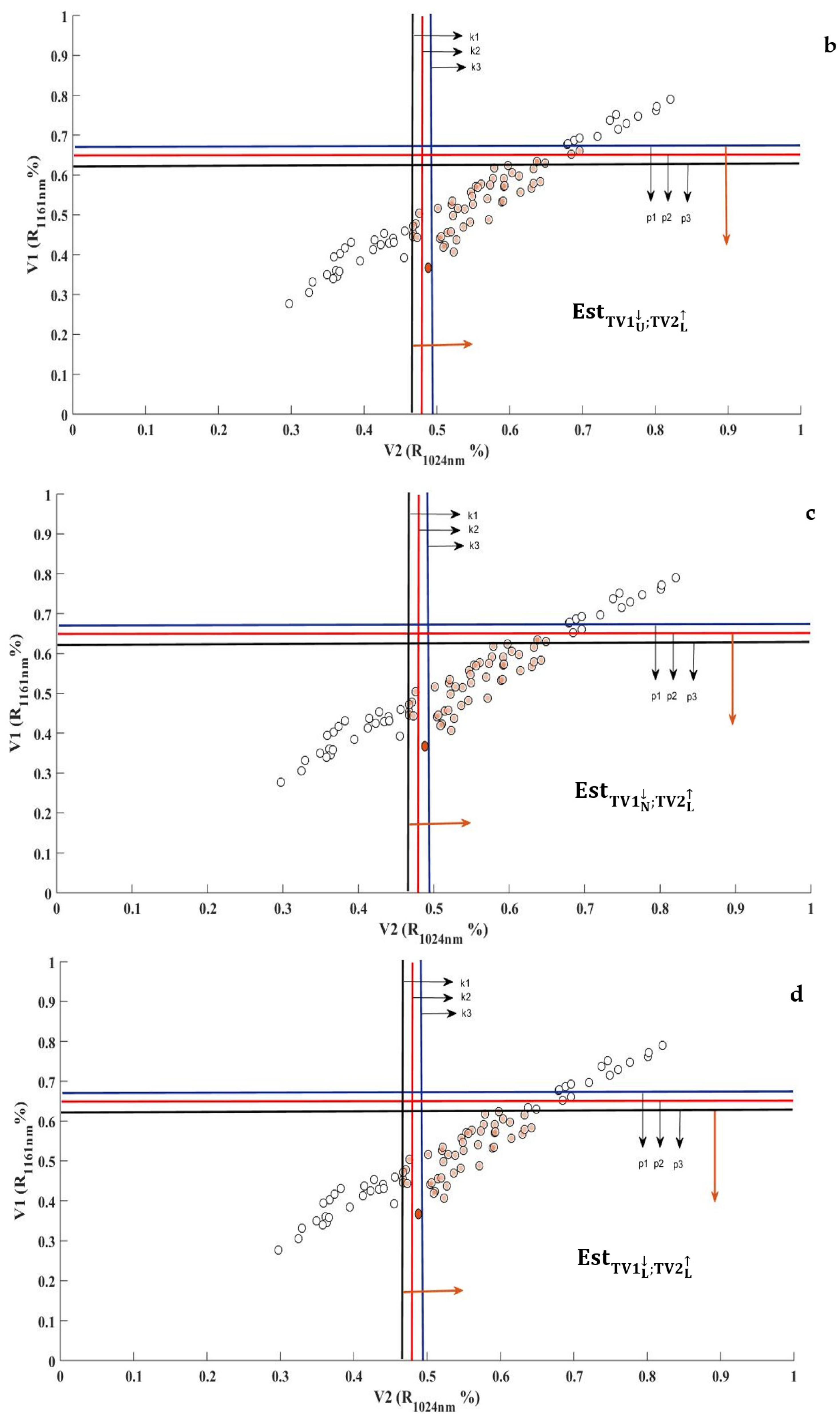
2.2.2. Development of the Ensemble-Based System

In order to optimize density estimates using the HM, the sources of uncertainty in classification and estimation must be controlled. For this purpose, we have developed a mixed EBS comprising both classifiers and ensemble-based estimators.
Parameterization of classifiers based on ensembles
The classification thresholds of the HM proposed by the CART algorithm are optimal, but not unique. A simple change in the training database leads to changes in the decision hierarchy. An effective way to control this error is to quantify the threshold uncertainties of the classifiers and to take them into account when estimating the density. Quantifying classifier uncertainty is possible using the bagging algorithm [33] (n-sampling with replacement; nbagg was set to 25,000), which is one of the most commonly used algorithms to build EBSs [28]. It consists of randomly removing a part of the calibration database and to compute a new classifier using the remaining data using the CART algorithm. The result of each iteration is the calculation of a threshold. The end of this step is marked by the development of two random vectors (v1) and (v2) composed of “n = 25,000” classifiers. The appearance of the thresholds composing the random vectors made it possible to determine a threshold probability distribution for each of the discrimination variables of the HM classifier. This probability is characterized by a mean (μ) and a variance (σ). These two statistical moments are subsequently used to develop the ensemble-based classifier consisting of a nominal (N), lower (L) and upper (U) threshold. Based on these statistical moments, it was possible to quantify the classification uncertainty by using the following equations:
Mean : μ f ( v ) = V · f ( v ) . · P ( v ) · dv
Variance : σ f ( v ) = V · ( f ( v ) μ ) 2 . · P ( v ) · dv
where v is the random vector belonging to V, which represents the space of the input variables of the model, f(v) is the output of the model and P(v) is the conditional distribution of the input variables.
Normally, all classification decisions made by the ensemble-based classifier should be retained and the most frequent decision is considered the correct one [28]. This process minimizes the risk of snow sample misclassification. However, taking into account each output of ensemble-based classifiers to make a decision for each processed sample will surely require a huge processing time. Tørvi and Hertzberg [30] proposed an approach based on the GQF, which converts the probabilistic integrals (Equations (1) and (2)) into weighted summations (Equations (3) and (4)), which are functions of the original distribution’s optimal n-thresholds (nOT). Each Optimal threshold (OT) is weighted according to its occurrence in the random vector (Table 1), fixed at three in our study. Table 1 summarizes the abscissa and weights related to each OT as proposed in the work of Tørvi and Hertzberg [30], where the mathematical details of the GQF demonstration and its validation can also be found. Thus, Equations (1) and (2) take the following forms:
Mean : μ = i = 1 n OT   ω i ×   f   ( z i )
Variance :   σ = i = 1 n OT   ω i ×   f   ( z i   μ ) 2
OTi = μ + σ × Z i
where μ and σ are respectively the empirical mean and variance of the standardized random vector f(z). Zi and ωi are respectively the abscissa and weight related to each optimal threshold (OTi; (i = 1: nOT)), nOT = 3.
Parameterization of estimators based on ensembles
Due to the complexity of the phenomenon to be modelled, the average of several density estimates will reduce the risk of using a single estimation function. Based on this principle and on the results of the ensemble classifier, it is possible to develop an ensemble estimator. Indeed, by means of the different thresholds calculated, it is possible to divide the calibration database into several sub-databases, allowing the calibration of 15 specific estimators, called “experts” in ensemble estimation [28]. Three subgroups of the WMM snow class, composed of the samples with the highest values (OTV1L, OTV1N, and OTV1U), nine subgroups of the MHM snow class, composed of samples in the middle range, and three subgroups of snow class HVM, composed of samples with the lowest values (OTV2L, OTV2N, and OTV2U; Figure 5). On the other hand, it has been shown that estimators based on multivariate regression improve the accuracy of the estimation. Expert calibration was therefore carried out using a stepwise regression. One of the great advantages of these experts is that they are not only specific to the class to be modelled, but also to the transition zones from one class to another, which are often problematic to model. This step marks the development of the ensemble-based estimator. Using this scheme, Equations (3) and (4) take the following form:
μ = i = 1 P ω i × Est OTV 1 i + i = 1 n OT P ω i × ( j = 0 k ω i   ×   ( Est OTV 1 i , OTV 2 j ) + j = 0 k ω i   ×   ( Est OTV 2 j , OTV 1 i )   ) ;   j = 0   for   k = 0
σ = i = 1 P   (   ω i × Est OTV 1 i   μ   )   2   + i = 1 n OT P ω i × ( j = 0 k ω i   × ( Est OTV 1 i , OTV 2 j   μ   ) 2 + j = 0 k ω i   ×   ( Est OTV 2 j , OTV 1 i   μ ) 2   ) ;   j = 0   for   k = 0
where i and j respectively indicate OTV1 and OTV2 (i = 1: nOT and j = 1: nOT; and where 1 refers to Lower (L), 2 refers to Nominal (N), and 3 refers to the Upper threshold (U); Figure 5); ωi and ωj are the weights associated with each particular optimal threshold for V1 and V2 (ω1 = ω3 = 1 6 and ω2 = 2 3 ; Table 1); V1 and V2 are the discrimination variables computed by the CART method; OTV1i and OTV2j are the optimal thresholds calculated by the GQF for V1 and V2 (Equations (3) and (4)); Est OTV 1 i   is the set of estimators (nOT) trained by the subgroups of the WMM snow class; Est OTV 1 i , OTV 2 j is the set of estimators ( n OT 2 ) trained by the subgroups of the MHM snow class; Est OTV 2 j , OTV 1 i is the set of estimators (nOT) trained by the subgroups of the snow class HVM; and k and p are the indices of the OT related to V1 and V2, respectively (k ≤ nOT and p ≤ nOT). More details are available in Appendix A.

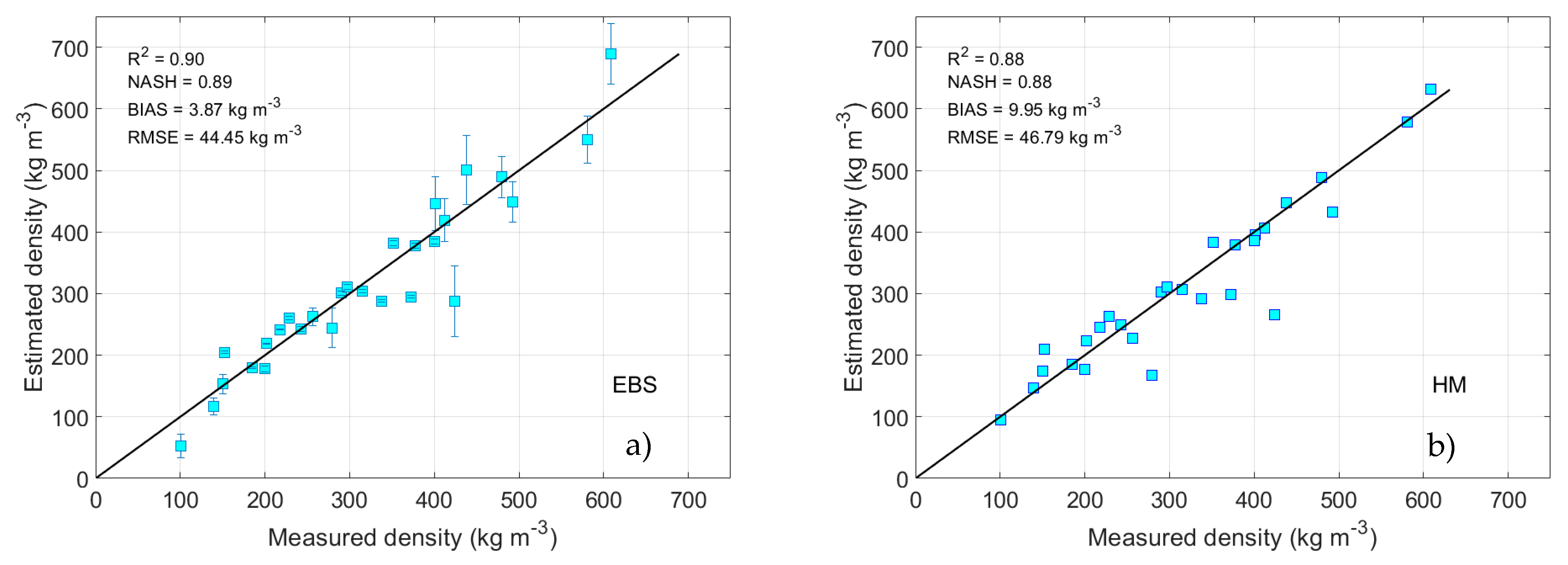
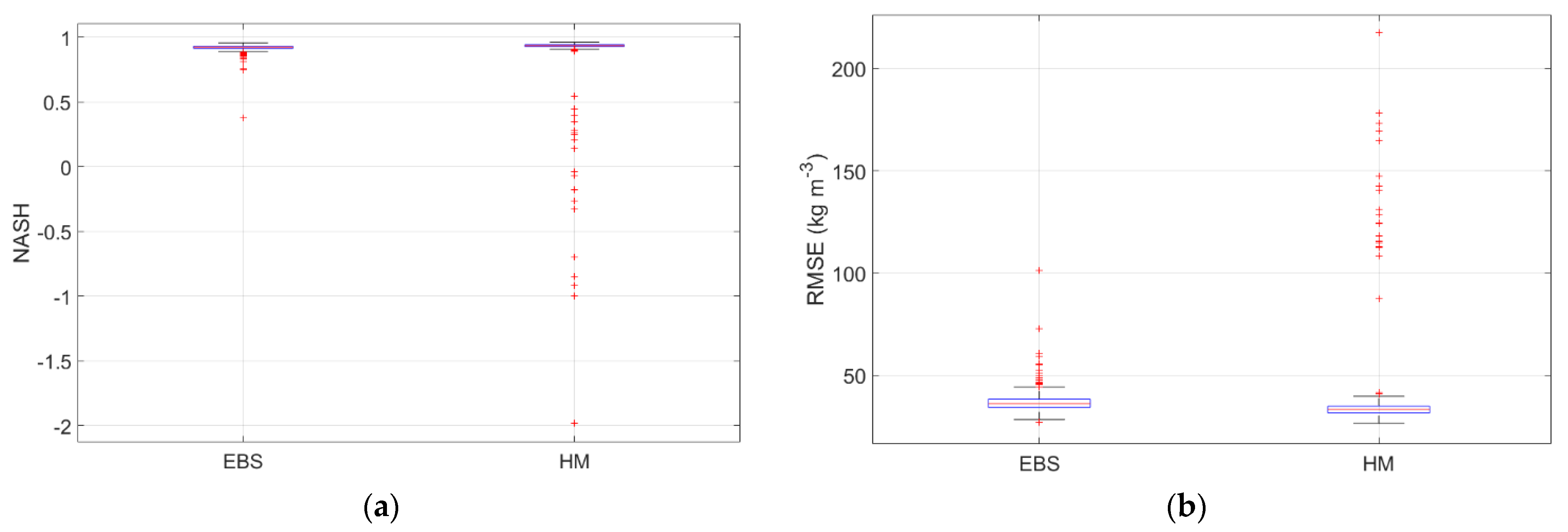
2.3. Accuracy Assessment

Twenty-five percent of the data was systematically selected from the initial database before proceeding to the EBS calibration (every fourth value was selected and set aside starting with low density values). This technique is called systematic split validation. The remaining data were used to calibrate the models by combining an ensemble-based classifier using CART with a multivariate stepwise regression based on fifteen specific estimators. The two models developed were subjected to a robustness test using the k-fold cross-validation method with 1K iterations. The latter is an iterative method (1K times) of random sampling by discount (50% of the data used for calibration and 50% for testing). The k-fold cross-validation approach is summarized in the flow chart in Figure 6.
The four statistical indices (Equations (8)–(11)) used to assess the EBS are: coefficient of determination (R2), BIAS, Root mean square error (RMSE), and Nash–Sutcliffe efficiency (NASH). The NASH criterion assesses performance based on the estimated values and the mean of the in situ measurements. A negative NASH value indicates that the mean of the measurements is more accurate than the model estimates; a NASH value of 1.0 means that the model is perfect [34]. The mathematical equations for the statistical indices used are as follows:
R 2 = [ i = 1 n ( M i M ¯ ) ( Es Es ¯ ) i = 1 n ( M i M ¯ ) 2 i = 1 n ( Es i Es ¯ ) 2 ] 2
RMSE = 1 n i = 1 n ( Es i M i M i ) 2
BIAS = 1 n i = 1 n   ( Es i M i M i )
NASH = 1 i = 1 n ( Es i M i M i ) 2 i = 1 n ( M i M ¯ M ¯ ) 2
where: n is the size of the dataset, M and Es are the measured and estimated density values and M ¯ and Es ¯ are the measured and estimated means.

3. Results and Discussion

3.1. Analysis of In Situ Snow Data

Twenty-four snow cores were collected from 19 January to 27 March 2018, from 10 January to 3 April 2019 and from 29 January to 9 March 2020. A total of 114 homogeneous layer samples were collected. In situ snow sample values are grouped by grain size, grain type, and density in Table 2, which highlights their variability [15]. On the basis of these three physical characteristics, each snow layer was associated to one of three snow classes (WMM, MHM, and VHM) based on the classification of Pahaut [35] and the International Classification of Seasonal Snow on the Ground of Fierz [31].

3.2. Estimator Calibration

By combining the results of the ensemble-based classifiers and estimators, it was possible to achieve a good level of diversity for both parameters since the final snow density estimate is based on at least three classifiers and three estimators (depending on the snow class to be modelled; Equation (6)). The dataset was separated into 15 subgroups, allowing training of 15 specific ensemble-based estimators. Calibration characteristics for the specific estimators are shown in Table 3. The correlation between spectral indices and in situ density measurements ranged from modest (R2 = 0.77 for specific estimators 13 and 14) to high (R2 = 0.97 for estimator 3). It is important to note that the specific estimators designed to estimate the three snow classes (WMM, MHM and HVM) were trained using linear functions.
It is known that the spectral reflectance of the snow cover results from the effect of different parameters, such as the metamorphism, grain size, grain shape, liquid water content, contamination, snow depth, etc. [36,37,38]. Indeed, the natural aging process of snow significantly affects the size, shape and cohesion of snow grains [39], which in turn influences reflectance. The specific estimators were analyzed to identify the wavelengths sensitive to each snow class, which were then used to estimate snow cover density using spectral data. Negi, et al. [40] showed that for changes in liquid water content, grain size and aging (metamorphism) of snow, the greatest spectral variations are observed between 980 and 1160 nm. Eppanapelli [41] suggested that the spectral reflectance of snow in the NIR is inversely proportional to the liquid water content in snow by using the normalized difference water index (NDWI) at 980 nm and 1310 nm. Gallet [16] used the NIR spectrum to determine the size of snow grains. They found that the 1310 nm wavelength, which corresponds to the central section of the NIR spectrum, is sensitive to small snow grains (low to medium density) and that the 1550 nm wavelength, which corresponds to the higher section of the NIR spectrum, is sensitive to large snow grains (denser).
Our results support the works cited above. Because of snow grain aging (high metamorphosis) and the high liquid water content of the HVM snow class, the shorter wavelengths of the NIR spectrum (979 nm and 974 nm) were the most sensitive wavelengths. We found that the reflectance of short wavelengths of the NIR spectrum is highly correlated with snow grain aging and liquid water content, and this is consistent with the works of Negi, Singh, Kulkarni and Semwal [40]. However, for specific estimator 15 (Table 3), which represents the transition class from high to moderate densities, wavelengths corresponding to the medium and long wavelengths of the NIR spectrum (1122 nm and 1441 nm) were the most sensitive. The wavelengths sensitive to the snow classes of low and medium density (WMM and MHM), were a mixture of short (968 nm, 946 nm, and 941 nm), medium (1172 nm), and long (1452 nm, 1617 nm and 1589 nm) wavelengths. This result was somewhat expected as both the WMM and MHM snow classes are composed of low, medium, and high-density snow blends, representing the different physical characteristics of the aging snow in terms of metamorphosis, liquid water content, and snow grain size and shape.

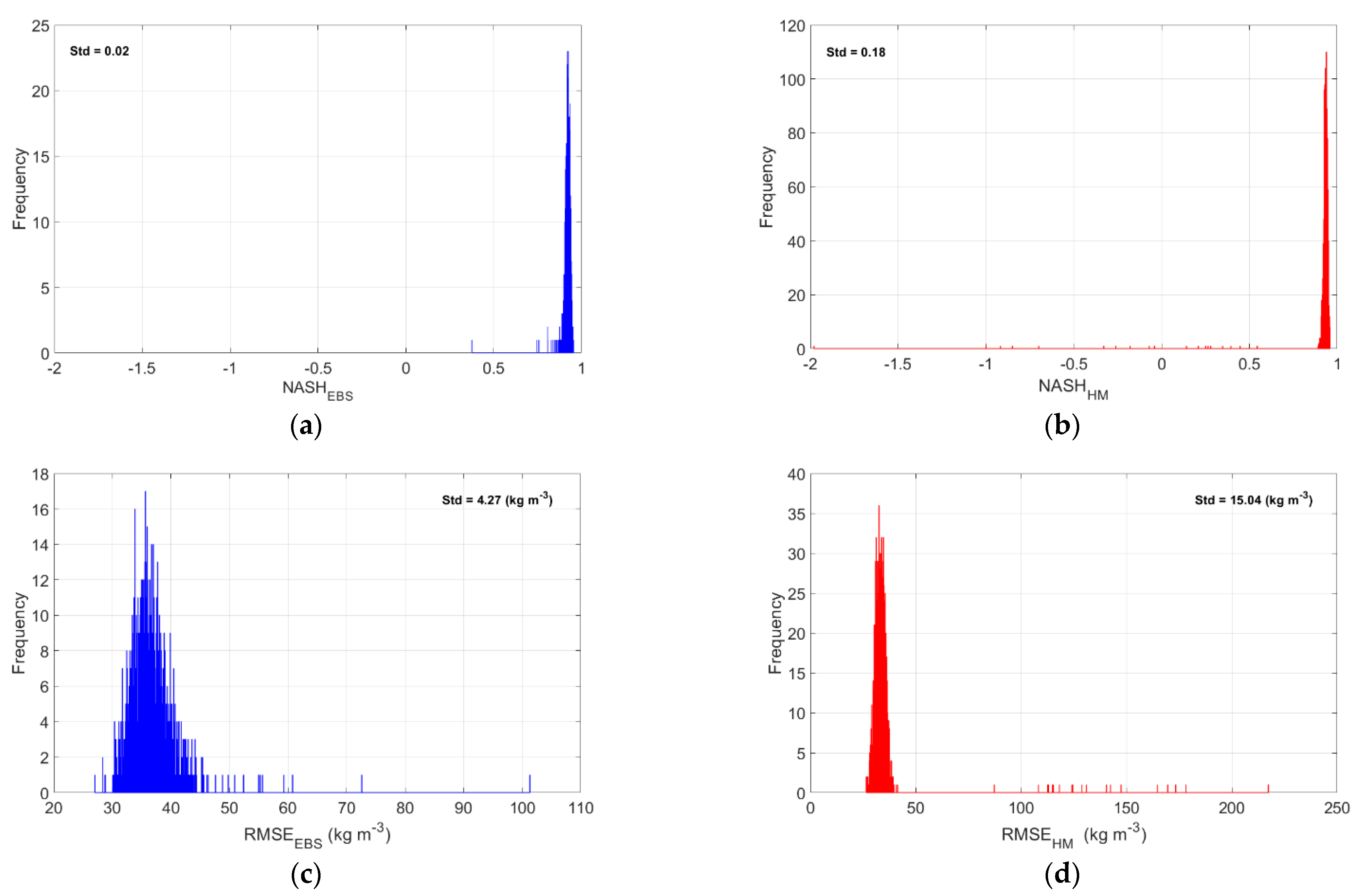
3.3. Evaluation and Validation of the Ensemble-Based System

Validation results obtained with the independent database demonstrate the potential of the EBS as an effective approach for estimating seasonal snowpack density. The performance of the EBS and the HM are compared in Figure 6. The EBS had a coefficient of determination of 0.90, which indicates that it explains up to 90% of the variance in the data. The NASH index indicates that the model is robust with an 89% success rate. The NASH is in fact a more robust statistical index than R2, as it compares the estimates to the mean of the observed measurements and is therefore not influenced by extreme values. An RMSE of 44.45 kg m−3 for such a range of densities is a very acceptable error. The slightly positive BIAS indicates that the EBS tends to overestimate the snow density. The robustness of the EBS was also confirmed by the scatterplot of the in situ measurements against their estimates (Figure 7), where all points are well distributed with respect to the 1:1 line. In summary, the EBS performs similarly to the HM.
It is important to note that for both the HM and EBS models (Figure 7a and b, respectively) we use the same independent database. The general conceptualization of the HM is based on a local classifier and a single specific estimator to calculate the density. In contrast, the EBS is based on a more general and stable classifier, and a combination of several specific estimator outputs driven by different NIR spectral regions (short, medium, and long wavelengths). Indeed, HM modelling is carried out in two steps: (1) classification of the snow samples and (2) estimation of the density of the classified snow samples using the corresponding specific estimator. Any misclassification error could lead to the selection of the wrong specific estimator, and consequently to an over- or underestimation of the density. An important advantage of the EBS is that the classification errors inherent to the HM are reduced and controlled. It is important to note that it is the way in which snow density is estimated with EBS that makes it more robust. Indeed, EBS modelling is based on the results of several experts trained with different spectral regions, hence their diversity. Thus, for each estimate, if all the experts converge toward the same density values using different spectral regions, this increases the estimation accuracy. On the other hand, even if one of the experts estimates the density incorrectly, averaging its result with those of the other experts allows controlling and minimizing of this error. In fact, according to Polikar [28], the averaging may or may not beat the performance of the best classifier in the ensemble, but it certainly reduces the overall risk of making a particularly poor selection.

3.4. Reliability Test

The two developed approaches have undergone a robustness test using the k-fold cross-validation method with 1K iterations. The objective of this test is to quantify the stability and reliability of the two approaches to provide a good estimate of snow density using the bagging technique. The latter is an iterative (1K times) random sampling method by discounting (50% of the data used for calibration and 50% for testing). As expected, the EBS showed great flexibility in providing quality estimates of snow density compared to the HM. The histogram spreads (NASH and RMSE) of the EBS are less wide than those of the HM (Figure 8). This behavior reflects the high robustness and reliability of the EBS (stdNASH = 0.18 and stdRMSE = 15.04 kg m−3 versus stdNASH = 0.02 and stdRMSE = 4.27 kg m−3 for the HM and EBS, respectively). Furthermore, the boxplot results support the histogram results. The boxplots (NASH and MSE) for the MBME are narrower with less data falling outside the normal (boxplot) which means that the values, whether NASH or RMSE, belong to the same population, in other words, the EBS estimates for the 1K iterations do not vary much. This is in contrast to the HM results, where we notice more values that fall outside the boxplot and therefore reflect the non-robust nature of the HM (Figure 9).
The EBS is based on a more general classifier and a combination of several specific estimator outputs driven by different NIR spectral regions (short, medium, and long). This conceptualization mitigates any potential misclassification error, unlike that of the MH, leading to the selection of a wrong specific estimator, and consequently to an overestimation or underestimation of the density. On the other hand, since the EBS outputs are based on a set of experts, it is also possible to associate a confidence interval for each estimate, which is neither the case for the HM nor for the standard models.

4. Conclusions

In this paper, we proposed to use an EBS to estimate the seasonal snowpack density. We used NIR hyperspectral data (900–1700 nm) at a spectral resolution of 5.5 nm. The EBS was developed to control and attenuate the uncertainties associated with the HM. To enhance the reliability of our approach, we created a set of classifiers and estimators. Several innovative aspects were developed in this approach: (1) the use of in situ physical and optical data collected weekly for three winters (2018–2020); (2) the use of an EBS for classification and regression purposes in a proximal remote sensing application, and (3) the use of GQF for runtime optimization. The combination of these points led to the development of a robust method capable of estimating seasonal snowpack density and monitoring its continuous evolution.
The validation technique used to assess the performance of our approach was based on the use of an independent database. The results of the validation with the independent database were satisfactory, with NASH = 0.89 and R2 = 0.90, despite some relatively low-density values (90–120 kg m−3). However, the validation process showcased that the EBS underestimated density values. Since this is a systematic error, it could be corrected during the modelling process.
This work can be a real step forward in identifying and monitoring the different processes that lead to the continuous evolution and regular control of seasonal snow accumulations. Indeed, such a prospect opens the way for the future implementation of multispectral or hyperspectral PIR systems, capable of measuring the density of the vertical stratigraphy of a wide variety of snowpacks (low and high elevation open and closed environments, coastal and continental conditions, mountains, etc.) at high vertical resolution and large scale of snowpack densities, without the need to dig snow pits. The system can also be used for a variety of scientific studies ranging from simple comparative analysis to more in-depth statistical investigations.
The proposed method allows retrieval of robust and accurate density estimates due to the very fine spectral resolution of the NIR hyperspectral sensor. However, the EBS approach is not limited to the NIR spectrum and could be applied to data from any other optical sensor, as high spectral resolution sensors become increasingly available. This new modelling approach could be of great help to water managers in northern regions, by optimizing snow water equivalent estimation. Another application would be to support researchers in their works aimed at understanding the spatio-temporal dynamics of seasonal snowpack’s and their metamorphic evolution. The results of the EBS are comparable to those of the HM, but its robustness and accuracy could motivate its preferred use. Another interesting feature is that our system can be easily customized by the addition of other components and classifiers.

Author Contributions

Conceptualization, M.K.E.O. and K.C.; methodology, M.K.E.O., A.E.A. and K.C.; writing—original draft preparation, M.K.E.O.; writing—review and editing, M.K.E.O., A.E.A. and M.B.; supervision, K.C. and A.E.A. All authors have read and agreed to the published version of the manuscript.

Funding

This research received no external funding.

Institutional Review Board Statement

Not applicable.

Informed Consent Statement

Not applicable.

Data Availability Statement

Not applicable.

Acknowledgments

Many people have reviewed and commented on the drafts of this document. The comments of A.E.A. and M.B. were particularly appreciated. Karem Chokmani’s encouragements were very helpful, as was his valuable guidance. The preparation of this manuscript, the retrieval, measurement and photography of snow profiles and my work on snow metamorphism have been supported over the years in developing this work. Many thanks to Sophie Roberge and David Ethier for their efficient coordination of the field campaign.

Conflicts of Interest

The authors declare that they are submitting the manuscript to the journal without any known conflict of interest.

Appendix A

An example of the subgroup selection used to calibrate the specific estimators for the brown point case in Figure A1. The arrows represent the direction of selection for each optimal threshold used.
The example presented here illustrates the steps taken to select the subgroups used to calibrate the submodels involved in estimating the density under a given physical metamorphosis condition. For example, if we take the case of the brown point on the graph below, p and k will be equal to 3. Thus, Equations (6) and (7) will take the following forms:
μ = 1 6 × Est TV 2 U + 1 6 × ( 1 6 × Est TV 1 U ; TV 2 L + 2 3 × Est TV 1 N ; TV 2 L + 1 6 × Est TV 1 L ; TV 2 L ) + 2 3 × ( 1 6 × Est TV 1 U ; TV 2 N + 2 3 × Est TV 1 N ; TV 2 N + 1 6 × Est TV 1 L ; TV 2 N )
σ = 1 6 × ( Est TV 2 U   μ ) 2 + 1 6 × ( 1 6 × ( Est TV 1 U ; TV 2 L μ ) 2 + 2 3 × ( Est TV 1 N ; TV 2 L μ ) 2 + 1 6 × ( Est TV 1 L ; TV 2 L   μ   ) 2 ) + 2 3 × ( 1 6 × ( Est TV 1 U ; TV 2 N μ ) 2 + 2 3 × ( Est TV 1 N ; TV 2 N   μ   ) 2 + 1 6 × ( Est TV 1 L ; TV 2 N     μ   ) 2 )
where μ is the weighted average of the density estimate and σ is its variance and Est TV 2 U   (Figure A1a) is the expert calibrated with the subgroup of the training data set where the spectral index is below the upper optimal threshold of V2. Estimators Est TV 1 U ; TV 2 L (Figure A1b), Est TV 1 N ; TV 2 L (Figure A1c) and Est TV 1 L ; TV 2 L (Figure A1d) are the experts calibrated with the subgroups of training databases where the spectral indices are both above the lower optimal thresholds for V2 and below the lower, nominal, and upper optimal thresholds for Est TV 1 U ; TV 2 N (Figure A1e), Est TV 1 N ; TV 2 N (Figure A1f), and Est TV 1 L ; TV 2 N (Figure A1g) are the experts calibrated with the subgroups of training databases where the spectral indices are both above the nominal optimal thresholds for V2 and below the lower, nominal, and upper optimal thresholds for V1. This combination of experts is not unique, as it varies according to the snow classes to be modelled (p and k).
Figure A1. Scheme of training subgroup selection in one of the moderate snow class cases (brown points).
Remotesensing 14 01089 g0a1aRemotesensing 14 01089 g0a1bRemotesensing 14 01089 g0a1c

Appendix B

Figure A2. Flow chart of the developed algorithm for density estimation (Samp is the number of samples; OTV1 and OTV2 refer to the optimal thresholds of V1 and V2 and Est are the specific estimators as described in Table 3).
Remotesensing 14 01089 g0a2

References

  1. Schweizer, J.; Bruce Jamieson, J.; Schneebeli, M. Snow avalanche formation. Rev. Geophys. 2003, 41, 4. [Google Scholar] [CrossRef] [Green Version]
  2. Gray, D.; Landine, P. An energy-budget snowmelt model for the Canadian Prairies. Can. J. Earth Sci. 1988, 25, 1292–1303. [Google Scholar] [CrossRef]
  3. McKay, G.; Blackwell, S. Plains snowpack water equivalent from climatological records. In Proceedings of the 29th Annual Western Snow Conference, Spokane, WA, USA, 11–13 April 1961; pp. 2–43. [Google Scholar]
  4. Matzl, M.; Schneebeli, M. Measuring specific surface area of snow by near-infrared photography. J. Glaciol. 2006, 52, 558–564. [Google Scholar] [CrossRef] [Green Version]
  5. Pielmeier, C.; Schneebeli, M. Stratigraphy and changes in hardness of snow measured by hand, ramsonde and snow micro penetrometer: A comparison with planar sections. Cold Reg. Sci. Technol. 2003, 37, 393–405. [Google Scholar] [CrossRef]
  6. Kinar, N.; Pomeroy, J. Measurement of the physical properties of the snowpack. Rev. Geophys. 2015, 53, 481–544. [Google Scholar] [CrossRef]
  7. Berisford, D.F.; Molotch, N.P.; Durand, M.T.; Painter, T.H. Portable spectral profiler probe for rapid snow grain size stratigraphy. Cold Reg. Sci. Technol. 2013, 85, 183–190. [Google Scholar] [CrossRef]
  8. Zuanon, N. IceCube, a portable and reliable instruments for snow specific surface area measurement in the field. In Proceedings of the International Snow Science Workshop, Grenoble-Chamonix, Mont-Blance, France, 7–11 October 2013; pp. 1020–1023. [Google Scholar]
  9. Domine, F.; Salvatori, R.; Legagneux, L.; Salzano, R.; Fily, M.; Casacchia, R. Correlation between the specific surface area and the short wave infrared (SWIR) reflectance of snow. Cold Reg. Sci. Technol. 2006, 46, 60–68. [Google Scholar] [CrossRef]
  10. Varade, D.; Maurya, A.K.; Sure, A.; Dikshit, O. Supervised classification of snow cover using hyperspectral imagery. In Proceedings of the 2017 International Conference on Emerging Trends in Computing and Communication Technologies (ICETCCT), Dehradun, India, 17–18 November 2017; pp. 1–7. [Google Scholar]
  11. ElMasry, G.; Sun, D.-W.; Allen, P. Near-infrared hyperspectral imaging for predicting colour, pH and tenderness of fresh beef. J. Food Eng. 2012, 110, 127–140. [Google Scholar] [CrossRef]
  12. Lorente, D.; Aleixos, N.; Gómez-Sanchis, J.; Cubero, S.; García-Navarrete, O.L.; Blasco, J. Recent advances and applications of hyperspectral imaging for fruit and vegetable quality assessment. Food Bioprocess Technol. 2012, 5, 1121–1142. [Google Scholar] [CrossRef]
  13. Lu, G.; Fei, B. Medical hyperspectral imaging: A review. J. Biomed. Opt. 2014, 19, 010901. [Google Scholar] [CrossRef]
  14. Donahue, C.; Skiles, S.M.; Hammonds, K. In situ effective snow grain size mapping using a compact hyperspectral imager. J. Glaciol. 2021, 67, 49–57. [Google Scholar] [CrossRef]
  15. El Oufir, M.K.; Chokmani, K.; El Alem, A.; Agili, H.; Bernier, M. Seasonal Snowpack Classification Based on Physical Properties Using Near-Infrared Proximal Hyperspectral Data. Sensors 2021, 21, 5259. [Google Scholar] [CrossRef]
  16. Gallet, J.-C.; Domine, F.; Zender, C.; Picard, G. Measurement of the specific surface area of snow using infrared reflectance in an integrating sphere at 1310 and 1550 nm. Cryosphere 2009, 3, 167–182. [Google Scholar] [CrossRef] [Green Version]
  17. Painter, T.H.; Molotch, N.P.; Cassidy, M.; Flanner, M.; Steffen, K. Contact spectroscopy for determination of stratigraphy of snow optical grain size. J. Glaciol. 2007, 53, 121–127. [Google Scholar] [CrossRef] [Green Version]
  18. Eppanapelli, L.K.; Lintzen, N.; Casselgren, J.; Wåhlin, J. Estimation of Liquid Water Content of Snow Surface by Spectral Reflectance. J. Cold Reg. Eng. 2018, 32, 05018001. [Google Scholar] [CrossRef]
  19. Negi, H.; Singh, S.; Kulkarni, A.; Semwal, B. Field-based spectral reflectance measurements of seasonal snow cover in the Indian Himalaya. Int. J. Remote Sens. 2010, 31, 2393–2417. [Google Scholar] [CrossRef]
  20. Gergely, M.; Schneebeli, M.; Roth, K. First experiments to determine snow density from diffuse near-infrared transmittance. Cold Reg. Sci. Technol. 2010, 64, 81–86. [Google Scholar] [CrossRef]
  21. El Oufir, M.K.; Chokmani, K.; El Alem, A.; Bernier, M. Estimating Snowpack Density from Near-Infrared Spectral Reflectance Using a Hybrid Model. Remote Sens. 2021, 13, 4089. [Google Scholar] [CrossRef]
  22. Alpak, F.O.; Vink, J.C.; Gao, G.; Mo, W. Techniques for effective simulation, optimization, and uncertainty quantification of the in-situ upgrading process. J. Unconv. Oil Gas Resour. 2013, 3, 1–14. [Google Scholar] [CrossRef]
  23. Chan, J.C.-W.; Paelinckx, D. Evaluation of Random Forest and Adaboost tree-based ensemble classification and spectral band selection for ecotope mapping using airborne hyperspectral imagery. Remote Sens. Environ. 2008, 112, 2999–3011. [Google Scholar] [CrossRef]
  24. Hansen, L.K.; Salamon, P. Neural network ensembles. IEEE Trans. Pattern Anal. Mach. Intell. 1990, 12, 993–1001. [Google Scholar] [CrossRef] [Green Version]
  25. Ismail, R.; Mutanga, O. A comparison of regression tree ensembles: Predicting Sirex noctilio induced water stress in Pinus patula forests of KwaZulu-Natal, South Africa. Int. J. Appl. Earth Obs. Geoinf. 2010, 12, S45–S51. [Google Scholar] [CrossRef]
  26. Jacobs, R.A.; Jordan, M.I.; Nowlan, S.J.; Hinton, G.E. Adaptive mixtures of local experts. Neural Comput. 1991, 3, 79–87. [Google Scholar] [CrossRef]
  27. Jordan, M.I.; Jacobs, R.A. Hierarchical mixtures of experts and the EM algorithm. Neural Comput. 1994, 6, 181–214. [Google Scholar] [CrossRef] [Green Version]
  28. Oza, N.C.; Tumer, K. Classifier ensembles: Select real-world applications. Inf. Fusion 2008, 9, 4–20. [Google Scholar] [CrossRef]
  29. Wang, S.-j.; Mathew, A.; Chen, Y.; Xi, L.-f.; Ma, L.; Lee, J. Empirical analysis of support vector machine ensemble classifiers. Expert Syst. Appl. 2009, 36, 6466–6476. [Google Scholar] [CrossRef] [Green Version]
  30. Polikar, R. Ensemble based systems in decision making. IEEE Circuits Syst. Mag. 2006, 6, 21–45. [Google Scholar] [CrossRef]
  31. Kelly, K.; Krzysztofowicz, R. A bivariate meta-Gaussian density for use in hydrology. Stoch. Hydrol. Hydraul. 1997, 11, 17–31. [Google Scholar] [CrossRef]
  32. Tørvi, H.; Hertzberg, T. Estimation of uncertainty in dynamic simulation results. Comput. Chem. Eng. 1997, 21, S181–S185. [Google Scholar] [CrossRef]
  33. Fierz, C.; Armstrong, R.L.; Durand, Y.; Etchevers, P.; Greene, E.; McClung, D.M.; Nishimura, K.; Satyawali, P.K.; Sokratov, S.A. The International Classification for Seasonal Snow on the Ground; UNESCO/IHP: Paris, France, 2009; Volume 25. [Google Scholar]
  34. Breiman, L.; Friedman, J.; Olshen, R.; Stone, C. Classification and Regression Trees; Springer: Monterey, CA, USA; Wadsworth, OH, USA, 1984. [Google Scholar]
  35. Breiman, L. Bagging predictors. Mach. Learn. 1996, 24, 123–140. [Google Scholar] [CrossRef] [Green Version]
  36. Nash, J.E.; Sutcliffe, J.V. River flow forecasting through conceptual models part I—A discussion of principles. J. Hydrol. 1970, 10, 282–290. [Google Scholar] [CrossRef]
  37. Pahaut, E. Les Cristaux de Neige et Leurs Métamorphoses; Direction de la Météorologie Nationale: Sarcenas, France, 1975. [Google Scholar]
  38. Dozier, J. Spectral signature of alpine snow cover from the Landsat Thematic Mapper. Remote Sens. Environ. 1989, 28, 9–22. [Google Scholar] [CrossRef]
  39. Warren, S.G. Optical properties of snow. Rev. Geophys. 1982, 20, 67–89. [Google Scholar] [CrossRef]
  40. Wiscombe, W.J. Improved Mie scattering algorithms. Appl. Opt. 1980, 19, 1505–1509. [Google Scholar] [CrossRef] [PubMed]
  41. Colbeck, S. An overview of seasonal snow metamorphism. Rev. Geophys. 1982, 20, 45–61. [Google Scholar] [CrossRef]
Figure 1. Geographical location of the sampling area.
Remotesensing 14 01089 g001
Figure 2. Snow core sampler.
Remotesensing 14 01089 g002
Figure 3. NIR spectral reflectance acquisition device for the vertical profile of snow samples from the company RESONON (Resonon Inc., Bozeman, MT, USA).
Remotesensing 14 01089 g003
Figure 4. Density class determination using the hybrid model. The light blue, the marine blue, and the dark blue dots indicate the WMM, MHM, and HVM classes, respectively, and represent the calibration database used to calibrate the corresponding estimators. The grey lines are the two discrimination thresholds used based on wavelengths V1 (1161 nm) and V2 (1024 nm).
Remotesensing 14 01089 g004
Figure 5. The two-dimensional GQF scheme using variables V1 and V2 and its application to calibrate the EBS. The black, red, and blue lines represent the optimal thresholds (lower, nominal, and upper, respectively) for V1 (OTV1L = 0.632, OT1N = 0.648 and OTV1U = 0.664) and V2 (OTV2L = 0.468, OTV2N = 0.480 and OTV2U = 0.492). k (1–3) and p (1–3) are the indices of the optimal thresholds associated with V1 and V2. The light blue, marine blue, and dark blue points represent the data used for training (WMM, MHM, and HVM, respectively) to calibrate the specific estimators. At the top right is the flow chart of the simplified EBS operational mode. The light blue, marine blue, and dark blue boxes designate the areas with WMM, MHM, and HVM classes, respectively. The overlapping areas in light and dark grey indicate the transitions between low-moderate and moderate-high densities, respectively. The terms of the equations are detailed in Equation (6). A detailed flow chart is presented in Appendix B.
Remotesensing 14 01089 g005
Figure 6. Stability test (k-fold cross-validation) flow chart.
Remotesensing 14 01089 g006
Figure 7. Snow density estimated by the two models (a) EBS and (b) HM compared to the in situ measurements for the independent database.
Remotesensing 14 01089 g007
Figure 8. Histograms showing the robustness test between EBS and HM: (a) standard deviation (NASHEBS) = 0.02, (b) standard deviation (NASHHM) = 0.18, (c) standard deviation (RMSEEBS) = 4.27 kg m−3, (d) standard deviation (RMSEHM) = 16.04 kg m−3.
Remotesensing 14 01089 g008
Figure 9. Boxplots representing the distribution of estimated snow density values expressed in (a) NASH and (b) RMSE, according to the two models EBS and HM.
Remotesensing 14 01089 g009
Table 1. Abscissa and weight of the optimal thresholds.
Optimal Threshold (OT)Abscissa (Zi) Weight   ( ω i )
101
2−1, +1 1 2 ,   1 2
3 3 ,   0 , + 3 1 6 ,   2 3 ,   1 6
Table 2. Distribution of snow density as a function of snow grain type and size (field data: 2018, 2019 and 2020 [15].
Snow ClassType of GrainGrain Size (mm)Number of Samples (N)Density (kg m−3)
WMM ( + λ ) <1 mm19100–250
MHM ( ) 1–2 mm59150–400
HVM ( ˄ ) >2 mm36350–650
Table 3. Calibration equations for each specific estimator. R2 is the coefficient of determination of the multivariate regressions; Samp is the size of the training dataset of each estimator; Exp var is the explanatory variable; U, N, and L are the Upper, Nominal and Lower thresholds; the arrow (↑) indicates an estimator trained with data superior to the threshold; and the downward arrow (↓) indicates an estimator trained with data inferior the threshold; the colors light blue, marine blue, and dark blue refer to the experts used to calculate the snow density of the WMM, MHM and HVM classes, respectively.
Snow ClassEstimator IDSpecific EstimatorCalibration EquationR2Samp Exp var   ( nm )
WMM1 Est TV 1 L −1119.75 × SISUB (1,282,941) − 167.590.91171282–941
2 Est TV 1 N −877.36 × SISUB (1,452,968) − 433.250.95151452–968
3 Est TV 1 U −967.69 × SISUB (1,666,935) − 425.240.97131666–935
MHM4 Est TV 1 U , TV 2 U −1491.40 × SINOR (1,600,946) − 951.090.83451600–946
5 Est TV 1 U , TV 2 N −1491.40 × SINOR (1,600,946) − 951.090.83451600–946
6 Est TV 1 U , TV 2 L −1432.65 × SINOR (1,617,946) − 880.870.84481617–946
7 Est TV 1 N , TV 2 U −1397.68 × SINOR (1,617,941) − 854.960.80431617–941
8 Est TV 1 N , TV 2 N −1397.68 × SINOR (1,617,941) − 854.960.80431617–941
9 Est TV 1 N , TV 2 L −1427.73 × SINOR (1,617,941) − 877.380.82461617–941
10 Est TV 1 L , TV 2 U −1480.06 × SINOR (1,600,946) − 940.110.80411600–946
11 Est TV 1 L , TV 2 N −1480.06 × SINOR (1,600,946) − 940.110.80411600–946
12 Est TV 1 L , TV 2 L −1419.73 × SINOR (1,617,946) − 868.750.82441617–946
HVM13 Est TV 2 U −26,859.26 × SINOR (979,974) + 82.900.7728979–974
14 Est TV 2 N −26,859.26 × SINOR (979,974) + 82.900.7728979–974
15 Est TV 2 L −1378.90 × SISUB (14,411,122) + 1207.810.86221441–1122
Publisher’s Note: MDPI stays neutral with regard to jurisdictional claims in published maps and institutional affiliations.

