Abstract
Multispectral (MS) pansharpening is crucial to improve the spatial resolution of MS images. MS pansharpening has the potential to provide images with high spatial and spectral resolutions. Pansharpening technique based on deep learning is a topical issue to deal with the distortion of spatio-spectral information. To improve the preservation of spatio-spectral information, we propose a novel three-stage detail injection pansharpening network (TDPNet) for remote sensing images. First, we put forward a dual-branch multiscale feature extraction block, which extracts four scale details of panchromatic (PAN) images and the difference between duplicated PAN and MS images. Next, cascade cross-scale fusion (CCSF) employs fine-scale fusion information as prior knowledge for the coarse-scale fusion to compensate for the lost information during downsampling and retain high-frequency details. CCSF combines the fine-scale and coarse-scale fusion based on residual learning and prior information of four scales. Last, we design a multiscale detail compensation mechanism and a multiscale skip connection block to reconstruct injecting details, which strengthen spatial details and reduce parameters. Abundant experiments implemented on three satellite data sets at degraded and full resolutions confirm that TDPNet trades off the spectral information and spatial details and improves the fidelity of sharper MS images. Both the quantitative and subjective evaluation results indicate that TDPNet outperforms the compared state-of-the-art approaches in generating MS images with high spatial resolution.
1. Introduction
Remote sensing images (RSIs) are broadly employed in different aspects, for instance, obtaining geographic data, obtaining earth resource information, hazard prediction and analysis, urban investigation, yield estimation and others [1]. However, in these applications, RSIs with high spatial, spectral or time resolution are usually required [2,3,4]. The spatial and spectral resolutions of RSIs constrain each other limited by sensor technology, i.e., panchromatic (PAN) images are with high spatial and low spectral resolutions, multispectral (MS) images are with low spatial and multispectral resolutions (LRMS) and hyperspectral (HS) images are with low spatial and high spectral resolutions [1,5]. The PAN images and MS or HS images need to be fused to produce high spatial resolution MS (HRMS) images or high spatial resolution HS (HRHS) images. This technique is also called panchromatic sharpening (pansharpening). Pansharpening for MS and PAN images is studied. Pansharpening methods can be approximately comprised of traditional approaches and deep learning (DL) methods [1,2,5]. Traditional approaches comprise the component substitution (CS) approach, multiresolution analysis (MRA) method and variational optimization (VO) technique [2,5].
CS methods first transform the MS images to other coordinate systems, and extract the spatial detail information. Then, the spatial detail information is substituted for the PAN image. Eventually, the substituted image is projected to the original coordinate system by inverse transformation to generate the HRMS image. Various CS methods have been developed, mainly including intensity-hue-saturation (IHS) [6], adaptive IHS (AIHS) [7], generalized IHS (GIHS) [8], Gram-Schmidt (GS) [9], GS adaptive (GSA) [1], Brovey [5] and partial replacement adaptive component substitution (PRACS) [10]. CS methods are simple and easy to implement, which greatly improve the spatial resolution of MS images. CS methods have the disadvantage of severe spectrum distortion and oversharpening.
MRA methods first decompose MS images and PAN images into images of different scales. Then, the corresponding scale images are fused by a fusion technique. Finally, an HRMS image is generated by an inverse transformation. The decomposition methods used generally include the discrete wavelet transform (DWT) [11,12], fusion for MS and PAN images employing the Induction scaling approach (Indusion) [13], generalized Laplacian pyramid (GLP) transform [14], modulation transfer function-GLP (MTF_GLP) transform [15], à trous wavelet transform (ATWT) [16], and other spectral and wavelet decomposition techniques [17,18,19]. MRA methods retain more spectral information and lessen the spectrum distortion. However, the spatial information is not rich and the resolution is lower.
The key to the VO method is to establish an energy function and optimization method [20,21,22,23]. Bayesian-based methods [24,25] and sparse representation-based methods [26,27,28,29] can also be classified into this category. Although the VO method can reduce spectral distortion, the optimization calculation is more complicated.
With the rapid development of DL, various types of convolutional neural networks (CNN)-based models are increasingly used in pansharpening and closely related tasks [30,31,32] of RSIs. Giuseppe et al. [33] proposed a CNN-based pansharpening method (PNN). PNN consists of only three layers and uses the nonlinear mapping of the CNN to reconstruct the LRMS image generating the HRMS image. The advantage of the PNN is that it has few layers and is easy to implement, but it also has the disadvantage of overfitting and limited expression ability. Wei et al. [34] put forward a deep residual network-based pansharpening technique (DRPNN). The DRPNN employs residual blocks to improve the fusion ability and reduce overfitting. Yang et al. [35] put forward a PanNet method based on residual modules and trained it in the frequency domain. To retain more spectrum information, add the upsampled MS image to the residual information. The model is trained in the frequency field to retain more spatial structure information, and the generalization ability of the network is better. Scarpa et al. [36] proposed a target-adaptive pansharpening means based on a CNN (TA-PNN). TA-PNN proposes a target-adaptive usage mode to deal with problems of data mismatch, multisensor data, and insufficient data. Liu et al. [37] designed a PsGan technique, which contains a generator and discriminator. The generator is a two-stream fusion structure that generates an HRMS image with MS and PAN images as inputs. The discriminator is composed of a full CNN to discriminate between the reference image and the produced HRMS image. Ma et al. [38] proposed a generative adversarial network-based model for pansharpening (Pan-Gan). Pan-Gan employs a spectral discriminator to discriminate the spectral information between the fused HRMS image and LRMS image. The spatial discriminator is employed to discriminate the spatial structure information between the HRMS and PAN images. Zhao et al. [39] designed an FGF-GAN method. The FGF-GAN generator uses a fast guided filter to retain details and a spatial attention module for fusion. FGF-GAN reduces network parameters and training time. Deng et al. [40] designed a CS/MRA model-based detail injection network (FusionNet). The injected details are acquired through the deep CNN based on residual learning, and then the upsampled MS image is added to the output of the detail extraction network. For FusionNet, the difference between the MS and PAN images (i.e., the duplicated PAN image of N channels, N is the channels of the MS image) is taken as the input. The multispectral information is introduced into the detail extraction network to lessen the spectral distortion. Wu et al. [41] designed a residual module-based distributed fusion network (RDFNet). RDFNet extracts multilevel features of MS images and PAN images, respectively. Then the corresponding level features and the fusion result of the previous step are fused to obtain the HRMS image. Although the network uses multilevel MS and PAN features as much as possible, it is affected by the depth of the network and cannot obtain more details and spectral information. Obviously, although various networks are used for pansharpening of RSIs and have acquired good results, there is rising space in terms of model complexity, implementation time, generalization ability, spectrum fidelity, retention of spatial details and so on.
In this article, we propose a novel three-stage detail injection network for pansharpening of RSIs by preserving spectral information to reduce spectral distortion and preserving details to strengthen spatial resolution. The main contributions of the work are as follows.
- A dual-branch multiscale feature extraction block is established to extract four-scale details of PAN images and the difference between duplicated PAN and MS images. The details are retained, and the MS image is introduced to preserve the spectrum information.
- Cascade cross-scale fusion (CCSF) employs fine-scale fusion information as prior knowledge for the coarse-scale fusion based on residual learning. CCSF combines the fine-scale and coarse-scale fusion, which compensates for the loss of information and retains details.
- A multiscale high-frequency detail compensation mechanism and a multiscale skip connection block are designed to reconstruct the fused details, which strengthen spatial details and reduce parameters.
- The quantitative evaluation and subjective evaluation of three satellite data sets are implemented at reduced and full resolutions.
2. Materials and Methods
2.1. Data Sets
To prove the performance of the designed pansharpening approach, three data sets are used for evaluation. The specific information of these data sets is as follows.
Gaofen-1 (GF-1) data set: These data are collected from Guangdong and Yunnan, China. The MS images have 4 bands. The resolutions of the PAN and MS images are 2 m and 8 m, respectively, and the radiometric resolution is 10 bits. The reduced resolution data are produced by Wald’s protocol [42], and the training samples, validation data and testing data are randomly selected. The number of data pairs in the data set is 21,560, 6160 and 3080, respectively. The number of full resolution testing data is 147.
QuickBird data set: These data are collected from Chengdu, Beijing, Shenyang and Zhengzhou, China. The MS images have 4 bands. The resolutions of the PAN and MS images are 0.6 m and 2.4 m, respectively, and the radiometric resolution is 11 bits. The number of training samples, validation data and testing data pairs is 20,440, 5840 and 2920, respectively. The number of full resolution testing data is 158.
Gaofen-2 (GF-2) data set: These data are collected from Beijing and Shenyang, China. The MS images have 4 bands. The resolutions of the PAN and MS images are 1 m and 4 m, respectively, and the radiometric resolution is 10 bits. The number of training samples, validation data and testing data pairs is 21,000, 6000 and 3000, respectively. The number of full resolution testing data is 286.
The sizes of the LMS (the reduced resolution form of the MS image), MS and (the reduced resolution form of the PAN image) images of the training data are 16 × 16 × 4, 64 × 64 × 4 and 64 × 64 × 1, respectively. The sizes of the MS and PAN images of the testing data at full resolution are 100 × 100 × 4 and 400 × 400 × 1, respectively.
2.2. Evaluation Indicators
The evaluation of pansharpening performance is performed at reduced and full resolutions. Subjective visual evaluation and objective evaluation are implemented on the experimental results. The objective evaluation indicators used in the reduced resolution experiment include the universal image quality index (UIQI) [43] extended to 4-band (Q4) [44], spectral angle mapping (SAM) [44], structural similarity (SSIM) [45], spatial correlation coefficient (SCC) [44] and erreur relative global adimensionnelle de Synthése (ERGAS) [44].
UIQI [43] assesses image quality from three sides: correlation, luminance and contrast. The representation of UIQI is Equation (1).
where g and f indicate the ground truth (GT) and pansharpened images, respectively. means the covariance between g and f images. and are the means and variance of g. and are the means and variance of f. The optimal value for UIQI is 1, and the pansharpening result is optimum.
The expression for Q4 [44] is Equation (2).
where and indicate the 4-band GT and pansharpened images, respectively. is the covariance between and . and are the means and variance of . and are the means and variance of .
SAM [44] is an error indicator, which represents the angle difference of spectral vector between the GT and pansharpened images. The expression of SAM is Equation (3).
where and are the spectrum vector of the GT and pansharpened images. SAM expresses the spectral distortion. When SAM = 0, the pansharpening performance is the best.
SSIM [45] represents the proximity of structural information between the GT and pansharpened images. SSIM is shown as Equation (4).
where and are constants. When SSIM = 1, the pansharpening result is the best.
SCC [44] represents the correlation of spatial details between the GT and pansharpened images. Spatial details are acquired through the high-pass filter. When SCC = 1, the pansharpened and GT images are most relevant.
ERGAS [44] is an error indicator, which shows the global effect of the pansharpened image. The representation of ERGAS is Equation (5).
where and indicate the spatial resolution of PAN and MS images, respectively. N is the number of bands. expresses the root mean square error of the bth band between the GT image and pansharpened image. indicates the mean of the bth band. The smaller the ERGAS, the better the pansharpening result. The optimum value for ERGAS is 0.
The objective evaluation indicators used in the full resolution experiment include the quality with no-reference (QNR), and [46].
denotes the spectrum distortion, the representation is Equation (6).
where and are the b-band and c-band low spatial resolution MS images, and are the b-band and c-band pansharpened images, and s is a positive integer to amplify the difference.
denotes the spatial distortion, the expression is Equation (7).
where p and mean the PAN image and degraded version of PAN image, and t is a positive integer to amplify the difference.
The representation for QNR [46] is shown as Equation (8).
where and are constants. When and , QNR is the largest and the pansharpening effect is the best. The optimum value for QNR is 1, and the ideal values for and are 0.
2.3. Implementation Settings
The implementation of the pansharpening network is the TensorFlow framework and a workstation containing an NVIDIA Tesla V100 PCIE GPU with 16 GB RAM and Intel Xeon CPU. The batch size is 32, and the number of iterations is . We employ the Adam optimizer [47] to optimize the pansharpening model, with the learning rate , , and . The channels of input and output of the network can be set according to the image channels used. The number of output channels of the network is 4 since the bands of MS and PAN are 4 and 1. To compare the pansharpening effect fairly, the CNN-based experiments are completed on the GPU, and the CS/MRA-based experiments are conducted in MATLAB on the CPU.
2.4. Network Structure
We propose a novel three-stage detail injection pansharpening network (TDPNet) for RSIs. Figure 1 represents the structure of TDPNet. Because of the lack of reference images, TDPNet is trained on the reduced resolution image. We employ the reduced resolution images LMS and of the MS and PAN images. The ↑LMS image is an upsampled LMS image, the same size as . MS represents the reference image, and H_MS indicates the generated pansharpening result. Here, m is the ratio of the resolution of the MS and PAN images. TDPNet includes three stages: a dual-branch multiscale detail extraction stage, cascade cross-scale detail fusion stage, and reconstruction stage of injecting details. The dual-branch multiscale detail extraction stage extracts multiscale details from the PAN image and ↑LMS image generating details of four scales. The first stage consists of two branches. One branch extracts multiscale details from the PAN image. The other branch extracts multiscale features from the difference image between the image (the image is duplicated N channels, where N is the channels of the LMS image.) and ↑LMS image. The second is a cascade cross-scale detail fusion stage. Cascade cross-scale fusion is achieved by combining fine-scale and coarse-scale fusion based on residual learning and prior information of four scales. Cascade cross-scale fusion employs the fine-scale fusion information as prior knowledge for the coarse-scale fusion to compensate for the loss of information caused by downsampling and retain details. The third is a reconstruction stage of injecting details. In this stage, the key information generated in the second stage is reconstructed. To compensate for the loss of information, we design a multiscale detail compensation mechanism. In addition, the fusion results generated in the cascade cross-scale fusion stage are used as the prior knowledge to reconstruct details (i.e., a multiscale skip connection block). This can strengthen spatial details and reduce parameters. Finally, the pansharpening result is produced by adding the reconstructed details to the ↑LMS image.
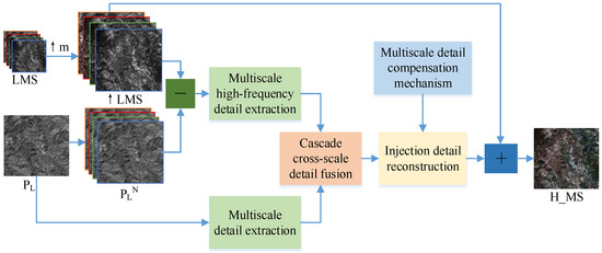
Figure 1.
The structure of the three-stage detail injection network for pansharpening.
2.4.1. Dual-Branch Multiscale Detail Extraction Stage
FusionNet [40] introduces the details of the difference between MS and PAN images, which has better performance than directly obtaining the details from the PAN image. Inspired by this approach, we propose a dual-branch multiscale detail extraction network. The composition of the network is shown in Figure 2. The proposed network is trained using the reduced resolution image and LMS image. One branch takes the difference between the ↑LMS and images as the input to obtain the high-frequency details of four scales. The introduction of MS details reduces the spectrum distortion and details distortion caused by the lack of relevant spectrum information in the PAN image. The details extracted by this branch are named composite high-frequency details (CHFDs). The other branch is to acquire the details of four scales of the image. In Figure 2, – represent the extracted CHFDs of four scales. – represent the extracted PAN details of the four scales.

Figure 2.
The dual-branch multiscale detail extraction network.
The conv module in Figure 2 adopts a residual learning block [48], and Figure 3 shows the structure. t represents the dimension of the input, and n represents the dimension of the output. In Figure 2, the sizes of the convolution kernels of the four conv modules are 3 × 3 × 32, 3 × 3 × 64, 3 × 3 × 128 and 3 × 3 × 256. The downsampling adopts the maximum pooling operation, and the sizes of the convolution kernels are 2 × 2 × 64, 2 × 2 × 128 and 2 × 2 × 256. The sizes of the and images are of those of the and images. The expressions for extracting the CHFDs are Equations (9)–(12).
where () shows the CHFDs of the jth scale, and are the reduced resolution images of the MS and PAN images, ↑ is an upsampled image, and ↑ presents the difference between MS and PAN images. represents the function of the direct connection part of the residual module. ∗ is a convolution operation. () represents the parameter of the direct connection part, and the convolution kernel size is 1 × 1, and the numbers are 32, 64, 128 and 256, respectively. expresses the residual part function of the residual module, () represents the parameter of the residual part, the convolution kernel size is 3 × 3, and the numbers are 32, 64, 128 and 256, respectively. indicates the function of the maximum pooling operation.
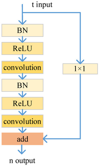
Figure 3.
Residual learning block.
The expressions for extracting details from the image are Equations (13)–(16).
where () means the PAN detail of the jth scale. () represents the parameter of the direct connection part, and the convolution kernel size is 1 × 1, and the numbers are 32, 64, 128 and 256, respectively. () represents the parameter of the residual part, the convolution kernel size is 3 × 3, and the numbers are 32, 64, 128 and 256, respectively.
2.4.2. Cascade Cross-Scale Detail Fusion Stage
This section describes the second stage of the TDPNet method, i.e., the cascade cross-scale detail fusion stage. The structure of this stage is shown in Figure 4. In this stage, the CHFDs and PAN details of four corresponding scales are concatenated, and then they are fused at the same scale. CCSF employs fine-scale fusion information as prior knowledge for coarse-scale fusion. CCSF is achieved by combining fine-scale and coarse-scale fusion based on residual learning and prior information of four scales. The representation of each content in Figure 4 is the same as the representation in Figure 2. First, the CHFDs and the PAN details are concatenated and then fused at the same scale to generate the prior fusion result . Then, the fine-scale fusion result provides the prior information for coarse-scale fusion. Cross-scale fusion ( and ) requires a scale transfer module to convert the fine-scale information into coarse-scale information. The scale transfer module used is a maxpooling operation, as shown in the red module of Figure 4. Then is downsampled and is generated. The and are fused, and the fusion result provides a priori information for the fusion of the next scale (i.e., ). In this way, the CCSF of four scales is carried out by combining the fine-scale and coarse-scale fusion, and finally, the key information is generated.
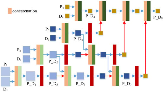
Figure 4.
Structure of the cascade cross-scale detail fusion network.
The expression of the cascade cross-scale detail fusion stage is Equation (17).
where shows the fused information of the cascade cross-scale detail fusion stage, indicates the function of the cascade cross-scale detail fusion network, and means the parameter.
2.4.3. Injection Detail Reconstruction Stage
This section is the third stage of the proposed TDPNet approach generating injection detail, i.e., the reconstruction stage of injection detail. The structure is shown in Figure 5. To compensate for the lost information, we design a multiscale high-frequency detail compensation mechanism. In addition, we take the fusion results generated in the cascade cross-scale fusion stage as a multiscale prior compensation module by multiscale skip connections. Finally, the pansharpening result is produced by adding the reconstructed injection detail to the ↑LMS image. This stage consists of three upsampling operations (i.e., deconvolution operation) and three convolutions after concatenating operations.

Figure 5.
The structure of the high-frequency details reconstruction network.
As shown in Figure 5, considering that some details will be lost in the downsampling process, to enhance the injection details generated by reconstruction, the fusion results of the first scale , the second scale and the third scale are introduced, forming multiscale skip connections. The multiscale skip connections not only reduce the network parameters but also compensate for the details. To further compensate for the information lost in the downsampling operations, we also design a multiscale high-frequency detail compensation mechanism, i.e., – in Figure 5. To match the scale of the reconstructed information, we design a scale transfer block for the compensation details. Figure 6 describes the structure diagram of the compensation details –. means the reduced form of the image. is obtained from the difference between and , and then two-scale details and are obtained by the downsampling operation. In this way, the detail compensation mechanism can further compensate for the information lost in the downsampling of the fusion stage and enhance the reconstruction details.
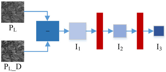
Figure 6.
Structure diagram for obtaining compensated details.
As shown in Figure 5, the result of CCSF undergoes a deconvolution operation, and convolution is performed after concatenating and , generating a finer scale image. After three such operations in turn, the final injection detail is generated. Finally, and ↑LMS images are added to obtain the pansharpening image.
The expression of obtaining the injection detail is Equation (18).
where presents the injection detail, d is the function of the three-stage injection detail extraction network, and indicates the parameter of the network.
The expression for pansharpening model TDPNet is Equation (19).
where indicates the generated pansharpening result.
The optimization objective of the pansharpening network TDPNet is the loss function, expressed as Equation (20).
where is the loss function, K indicates the number of training data in each iteration, and represents the reference image.
3. Results
To validate the pansharpening ability of the proposed TDPNet approach , the state-of-the-art CS/MRA-based techniques PRACS [10], Indusion [13] and MTF_GLP [15] and the CNN-based methods PNN [33], DRPNN [34], PanNet [35], FusionNet [40] and RDFNet [41] are employed for comparative experiments. The experimental results of reduced resolution, full resolution and evaluation indices on three data sets are as follows.
3.1. Experimental Results on GF-1 Data Set
This section describes the reduced and full resolution experiments on the GF-1 data set. Figure 7 shows the experimental results at reduced resolution of various comparison methods. Figure 7a shows a reduced resolution PAN (LPAN) image, and Figure 7b shows an upsampled reduced resolution MS image obtained by a polynomial kernel with 23 coefficients (EXP) [49]. The pansharpened results of the PRACS, Indusion, MTF_GLP, PNN, DRPNN, PanNet, FusionNet, RDFNet and TDPNet approaches are shown in Figure 7c–k, respectively. Figure 7l shows the reference MS image, i.e., the GT image. To conveniently observe the differences between various methods, we enlarge the red box area. To observe the pansharpening performance more conveniently, we also show the average intensity difference map and the average spectral difference map (calculated according to SAM) between the pansharpened result and the reference image, as shown in Figure 8 and Figure 9. We employ color to represent the difference, and the value gradually increases from blue to yellow. To highlight the difference, the values of the color bar of the average intensity difference map and the average spectral difference map are 0–0.5 and 0–1, respectively. The top row and the third row of Figure 8 and Figure 9 represent the difference map of the whole pansharpened result. The second row and the bottom row of Figure 8 and Figure 9 show an enlarged view of the corresponding region in the red box of Figure 7. Table 1 shows the quantitative evaluation indices of the experiment at reduced resolution.
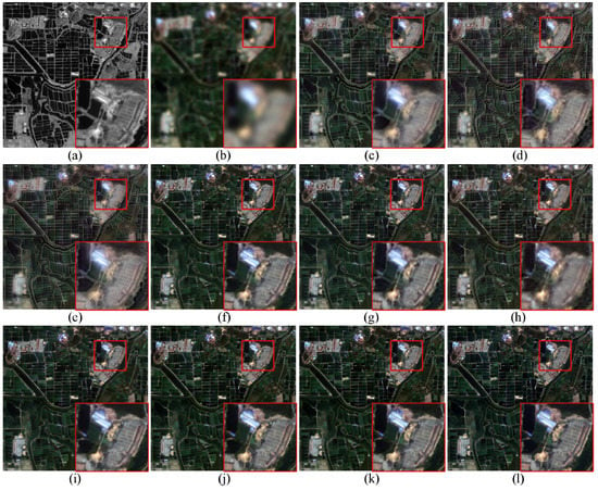
Figure 7.
The experimental results of various compared methods on GF-1 testing data at reduced resolution. (a) LPAN. (b) EXP. (c) PRACS. (d) Indusion. (e) MTF_GLP. (f) PNN. (g) DRPNN. (h) PanNet. (i) FusionNet. (j) RDFNet. (k) TDPNet. (l) Ground Truth.
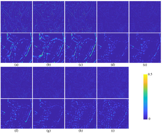
Figure 8.
The average intensity difference map between the generated image and GT on GF-1 testing data. The top row and the third row represent the difference map of the whole pansharpened result. The second row and the bottom row show the enlarged view of the corresponding region in the red box of Figure 7. (a) PRACS. (b) Indusion. (c) MTF_GLP. (d) PNN. (e) DRPNN. (f) PanNet. (g) FusionNet. (h) RDFNet. (i) TDPNet.
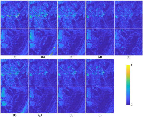
Figure 9.
The average spectral difference map between the fused image and GT on GF-1 testing data. The top row and the third row represent the difference map of the whole pansharpened result. The second row and the bottom row show the enlarged view of the corresponding region in the red box of Figure 7. (a) PRACS. (b) Indusion. (c) MTF_GLP. (d) PNN. (e) DRPNN. (f) PanNet. (g) FusionNet. (h) RDFNet. (i) TDPNet.

Table 1.
Quantitative evaluation of various compared methods on GF-1 testing data at reduced resolution.
From Figure 7, it is clearly found that the Indusion and MTF_GLP methods exhibit severe spectral distortion. The pansharpening results of the PRACS, Indusion, MTF_GLP and PanNet methods are relatively blurred. The pansharpening results of the PNN, DRPNN and FusionNet are also slightly vague compared to the GT image. RDFNet and the proposed method TDPNet have better pansharpening results. However, combined with Figure 8 and Figure 9, we find that the difference between TDPNet and GT is smaller, and the pansharpening result is better. In Table 1, the objective evaluation indices Q4, UIQI, SCC, SSIM and SAM of the proposed method are better. Although the ERGAS of the proposed method ranks second, it is only 0.0006 from the optimal value. The TDPNet is better in preserving spectrum information and details.
Figure 10 presents the experimental results at full resolution of each method. Figure 10a indicates the PAN image at full resolution, Figure 10b means the corresponding upsampled MS image, and the pansharpened results of the PRACS, Indusion, MTF_GLP, PNN, DRPNN, PanNet, FusionNet, RDFNet and TDPNet approaches are shown in Figure 10c–k, respectively. Table 2 presents the quantitative evaluation metrics of experimental results at full resolution. In the quantitative evaluation indices of the tables, black bold formatting indicates the best result.
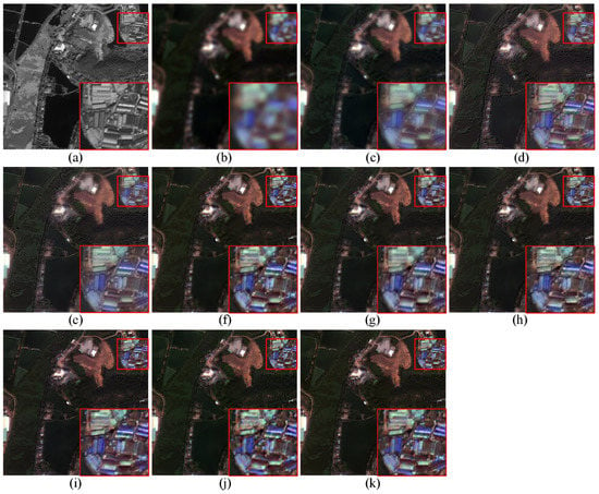
Figure 10.
The experimental results of various compared approaches of GF-1 testing image at full resolution. (a) PAN. (b) EXP. (c) PRACS. (d) Indusion. (e) MTF_GLP. (f) PNN. (g) DRPNN. (h) PanNet. (i) FusionNet. (j) RDFNet. (k) TDPNet.

Table 2.
Quantitative evaluation of various compared approaches on GF-1 testing data at full resolution.
From Figure 10, we can clearly find that the spectral distortions of PRACS, Indusion and MTF_GLP are relatively severe and that the MTF_GLP result is relatively fuzzy. Compared with the pansharpening results of other methods, the result of TDPNet is clearer and retains more spectral information. From Table 2, the objective evaluation indicators indicate that the of TDPNet is not the best; although PRACS and Indusion retain more details, their spectral distortions are more severe. The proposed method TDPNet has the best retention of spectral information, and the value of QNR is also optimal. Comprehensively, the pansharpening result of TDPNet is better than those of the other approaches.
3.2. Experimental Results on QuickBird Data Set
This section describes the experiment on the QuickBird data set. Figure 11 shows the experimental outcomes of the compared approaches at reduced resolution. Figure 12 and Figure 13 show the average intensity difference map and the average spectral difference map, respectively. Figure 14 shows the full resolution experimental results of the compared methods. Table 3 describes the quantitative evaluation indices of the experimental results at reduced resolution of the compared approaches. Table 4 presents the quantitative evaluation indices of the full resolution experimental results.
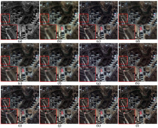
Figure 11.
The experimental results of various compared approaches on QuickBird testing data at reduced resolution. (a) LPAN. (b) EXP. (c) PRACS. (d) Indusion. (e) MTF_GLP. (f) PNN. (g) DRPNN. (h) PanNet. (i) FusionNet. (j) RDFNet. (k) TDPNet. (l) Ground Truth.
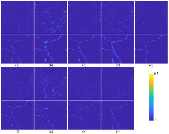
Figure 12.
The average intensity difference map between the fused MS image and GT on QuickBird testing data. The top row and the third row represent the difference map of the whole pansharpened result. The second row and the bottom row show the enlarged view of the corresponding region in the red box of Figure 11. (a) PRACS. (b) Indusion. (c) MTF_GLP. (d) PNN. (e) DRPNN. (f) PanNet. (g) FusionNet. (h) RDFNet. (i) TDPNet.
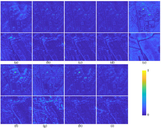
Figure 13.
The average spectral difference map between the fused image and GT on QuickBird testing data. The top row and the third row represent the difference map of the whole pansharpened result. The second row and the bottom row show the enlarged view of the corresponding region in the red box of Figure 11. (a) PRACS. (b) Indusion. (c) MTF_GLP. (d) PNN. (e) DRPNN. (f) PanNet. (g) FusionNet. (h) RDFNet. (i) TDPNet.
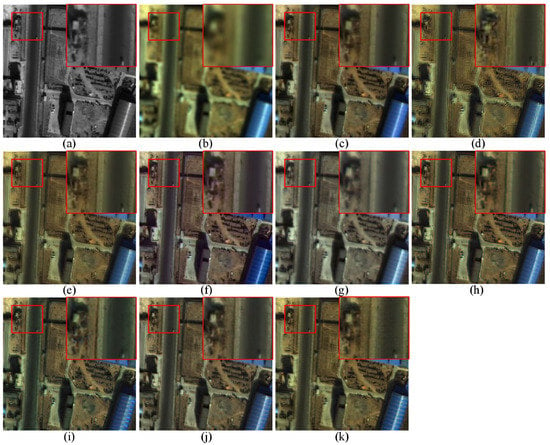
Figure 14.
The experimental results of various compared approaches on the QuickBird testing data at full resolution. (a) PAN. (b) EXP. (c) PRACS. (d) Indusion. (e) MTF_GLP. (f) PNN. (g) DRPNN. (h) PanNet. (i) FusionNet. (j) RDFNet. (k) TDPNet.

Table 3.
Quantitative evaluation of various compared approaches on QuickBird testing data at reduced resolution.

Table 4.
Quantitative evaluation of various compared approaches on QuickBird testing data at full resolution.
The pansharpening result of the DRPNN method in Figure 11 contain the most severe spectral distortion. Artifacts appear in the pansharpening result of the Indusion method. Combined with Figure 12 and Figure 13, the result shows that the proposed method retains more details while retaining spectral information. As shown in Table 3, the evaluation indices Q4 and SCC of TDPNet rank second. For Q4, the difference between TDPNet and RDFNet is very small. The proposed method TDPNet is the best for indicators UIQI, SCC, SSIM, SAM and ERGAS. The spectral distortion of the PNN and DRPNN in Figure 14 is severe. The result of the Indusion method exhibits artifacts and is relatively fuzzy. From Table 4, although the indices and of the proposed method TDPNet are both ranked second, TDPNet is the best in terms of retaining both spectral information and details simultaneously.
3.3. Experimental Results on GF-2 Data Set
This section describes the experiment on the GF-2 data set. Figure 15 shows the experimental results of the compared methods at reduced resolution. The average intensity difference map and the average spectral difference map are shown in Figure 16 and Figure 17. Figure 18 shows the full resolution experimental results of the compared methods. The quantitative evaluation indices of the experimental results at reduced resolution for the compared methods are shown in Table 5. The quantitative evaluation indices of the full resolution experimental results of each method are shown in Table 6.
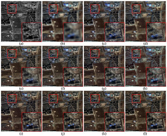
Figure 15.
The experimental results of various compared approaches on GF-2 testing data at reduced resolution. (a) LPAN. (b) EXP. (c) PRACS. (d) Indusion. (e) MTF_GLP. (f) PNN. (g) DRPNN. (h) PanNet. (i) FusionNet. (j) RDFNet. (k) TDPNet. (l) Ground Truth.

Figure 16.
The average intensity difference map between the fused MS image and GT on GF-2 testing data. The top row and the third row represent the difference map of the whole pansharpened result. The second row and the bottom row show the enlarged view of the corresponding region in the red box of Figure 15. (a) PRACS. (b) Indusion. (c) MTF_GLP. (d) PNN. (e) DRPNN. (f) PanNet. (g) FusionNet. (h) RDFNet. (i) TDPNet.
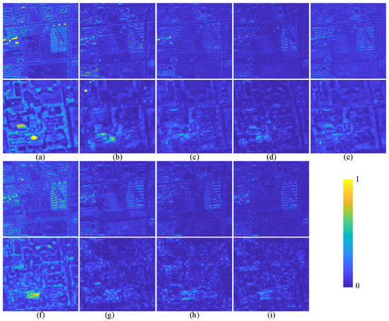
Figure 17.
The average spectral difference map between the fused image and GT on GF-2 testing data. The top row and the third row represent the difference map of the whole pansharpened result. The second row and the bottom row show the enlarged view of the corresponding region in the red box of Figure 15. (a) PRACS. (b) Indusion. (c) MTF_GLP. (d) PNN. (e) DRPNN. (f) PanNet. (g) FusionNet. (h) RDFNet. (i) TDPNet.
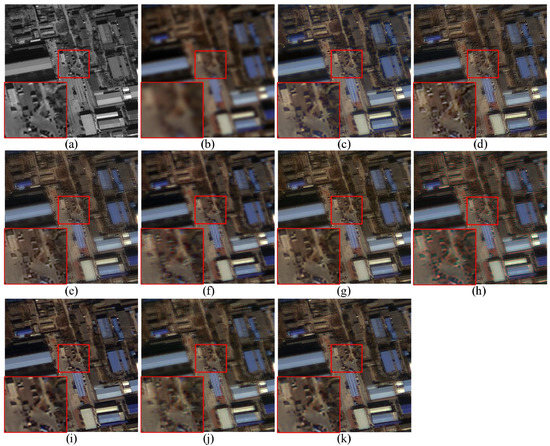
Figure 18.
The experimental results of various compared approaches on the GF-2 testing data at full resolution. (a) PAN. (b) EXP. (c) PRACS. (d) Indusion. (e) MTF_GLP. (f) PNN. (g) DRPNN. (h) PanNet. (i) FusionNet. (j) RDFNet. (k) TDPNet.

Table 5.
Quantitative evaluation of various compared approaches on GF-2 testing data at reduced resolution.

Table 6.
Quantitative evaluation of various compared methods on GF-2 testing data at full resolution.
The pansharpening results of PRACS and PanNet in Figure 15 exhibit the most severe spectrum distortion. The pansharpening result of Indusion is blurry. Combined with Figure 16 and Figure 17, the results show that the PNN, RDFNet and TDPNet methods retain more spectral information, whereas the TDPNet method retains more details. The objective indicators in Table 5, except SAM, indicate that the results of TDPNet are optimal. From the visual effect of Figure 18, the spectral distortion of PanNet is the most severe, and the results of the PNN and RDFNet methods are blurred. Although the index of Indusion in Table 6 is the best, the spectral distortion is severe. Although the index of PNN is the best, more spatial details are lost. Combined with the overall spectral distortion and the retention of spatial structure information, the pansharpening performance of the proposed method TDPNet is better than that of the other approaches.
3.4. Implementation Time
Table 7 shows the implementation time of pansharpening for the compared approaches at full resolution. The sizes of the MS and PAN images are 100 × 100 × 4 and 400 × 400 × 1, respectively. Note that the approaches based on CNN are realized on the GPU, and the approaches based on CS and MRA are realized on the CPU. Although the implementation time is not the shortest, it is acceptable for the CNN-based method.

Table 7.
Implement time (seconds) of pansharpening for compared methods.
4. Discussion
Based on the aforementioned experimental results, it is evidently found that the proposed TDPNet well trade off the contents of spectral and spatial. This section discusses the major compositions of TDPNet, the number of iterations and the consumed time in the training and testing processes.
4.1. Major Compositions of TDPNet
We discuss impacts of compositions of the three stages of the proposed TDPNet on the pansharpening performance from three main contents. The following discussion is based on the experimental results of the GF-2 data.
First, the dual-branch multiscale high-frequency detail extraction stage comprises two branches to extract the features of ↑ and images respectively. Verifying the effectiveness of features extracted from ↑ image, we compare the performance of the dual-branch with ↑ and images (i.e., TDPNet-n-p) with that of the dual-branch with ↑ and images (TDPNet). TDPNet-n-p extracts the four-scale information from ↑ and respectively, and the other parts are the same as TDPNet. The compared results are shown in Figure 19. We clearly observe that the pansharpening performance of TDPNet is better than that of TDPNet-n-p in terms of preserving spectral and spatial information.
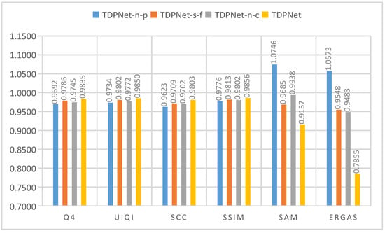
Figure 19.
The effect of the components of TDPNet on the pansharpening results of the GF-2 data.
Second, we use a basic fusion block (i.e., Figure 20, the contents are the same as that in Figure 4.) to replace the CCSF in the second stage, and the other parts are the same as TDPNet, which is called TDPNet-s-f. In Figure 19, it is found that the performance of TDPNet is significantly better than that of TDPNet-s-f, and cross scale fusion in CCSF enhances spatial details and spectrum information.
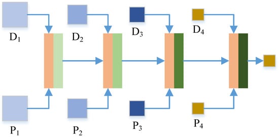
Figure 20.
A basic fusion block.
Third, we remove the multiscale high-frequency detail compensation mechanism of the third stage, and the other parts of TDPNet remain the same, which is termed TDPNet-n-c. In Figure 19, it is evidently observed that the result of TDPNet is finer than TDPNet-n-c. From Figure 19, the main parts of the three stages promote the pansharpening performance of TDPNet, enhancing spatial details and reducing spectral distortion.
4.2. Iterations and Consumed Time
The number of iterations of all the CNN-based approaches is obtained on the same data set. The number of iterations and consumed time for each approach achieving the optimal performance are demonstrated in Figure 21 and Figure 22. Note that the time spent on PanNet contains the time used to extract high-frequency details. In Figure 22, FusionNet [40] takes the least time reaching convergence because of the simple composition of it. Although the times of TDPNet reaching convergence is less, it spend longer time because of the relatively complex compositions of the network. In Figure 21 and Figure 22, compared with other CNN-based approaches, the time spent on TDPNet is acceptable. In the next research, we can further simplify the network structure by employing group convolutions and separable convolutions and design a lightweight pansharpening network, which takes less time while achieving the same or higher performance.
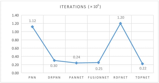
Figure 21.
The number of iterations of comparative approaches based on CNN.
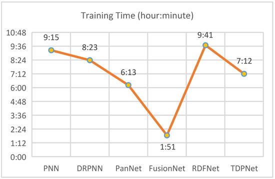
Figure 22.
Training time of comparative approaches based on CNN.
5. Conclusions
To improve the preservation of spatio-spectral information, we proposed a novel three stages detail injection network for remote sensing images pansharpening to reconstruct details. A dual-branch multiscale feature extraction block obtains four scale details of PAN image and the difference between duplicated PAN and MS images, respectively. This utilizes the abundant spatial details of the PAN images and retains the spectral information by introducing MS image. CCSF employs the fine-scale fusion information as prior knowledge for the coarse-scale fusion information compensating for the lost information during downsampling and retaining high-frequency details. The multiscale detail compensation mechanism and multiscale skip connection block compensate for the lost information and reduce parameters during reconstructing injection detail. Extensive experimental analysis on GF-1, QuickBird and GF-2 data sets both at degraded and full resolutions testify that TDPNet trades off the spectral information and spatial details and improves the fidelity of sharper MS images. The quantitative evaluation and subjective evaluation results indicate that TDPNet has better ability in retaining spectrum information and spatial details than the other compared approaches. Nevertheless, the implementation time of proposed TDPNet is not the least.
In the next research, we can further simplify the network structure and design a lightweight pansharpening network, which takes less time while achieving the same or higher performance. Besides, designing a lightweight pansharpening network with the same or better performance has the following advantages: (1) There is less requirement for the server during training. (2) Fewer parameters. (3) It is more suitable for implementing on devices with limited memory. Our future work also needs to optimize the network structure and design a lightweight pansharpening network by group convolutions and separable convolutions to decrease the implementation time and further boost the pansharpening ability.
Author Contributions
Conceptualization, Y.W.; methodology, Y.W.; software, Y.W.; validation, Y.W.; formal analysis, Y.W., C.L., H.Z. and M.H.; investigation, H.Z., C.L. and M.H.; resources, M.H. and S.F.; data curation, M.H. and S.F.; writing—original draft preparation, Y.W.; writing—review and editing, Y.W., H.Z., C.L., M.H. and S.F.; visualization, Y.W.; supervision, M.H. and S.F.; project administration, M.H.; funding acquisition, M.H. and S.F. All authors have read and agreed to the published version of the manuscript.
Funding
The work was encouraged by Hainan Provincial Natural Science Foundation of China under Grant 2019CXTD400, and the National Key Research and Development Program of China under Grant 2018YFB1404400.
Institutional Review Board Statement
Not applicable.
Informed Consent Statement
Not applicable.
Data Availability Statement
The data provided in this study can be provided at the request of the corresponding author. The data has not been made public because it is still used for further research in the study field.
Acknowledgments
Thanks for PNN codes in [33] supplied by Giuseppe Scarpa. Thanks for Wei and Yuan providing DRPNN codes in [34]. Thanks for PanNet codes in [35] provided by Yang, J. Thanks to Deng L. J. in [40] for providing FusionNet codes.
Conflicts of Interest
The authors declare no conflict of interest.
Abbreviations
The following abbreviations are used in this manuscript:
| MS | multispectral |
| TDPNet | three-stage detail injection pansharpening network |
| PAN | panchromatic |
| CCSF | cascade cross-scale fusion |
| RSIs | Remote sensing images |
| LRMS | low spatial and multispectral resolutions |
| HS | hyperspectral |
| HRMS | high spatial resolution MS |
| HRHS | high spatial resolution HS |
| pansharpening | panchromatic sharpening |
| DL | deep learning |
| CS | component substitution |
| MRA | multiresolution analysis |
| VO | variational optimization |
| IHS | intensity-hue-saturation |
| AIHS | adaptive IHS |
| GIHS | generalized IHS |
| GS | Gram-Schmidt |
| GSA | GS adaptive |
| PRACS | partial replacement adaptive component substitution |
| DWT | discrete wavelet transform |
| Indusion | fusion for MS and PAN images employing the Induction scaling approach |
| GLP | generalized Laplacian pyramid |
| MTF_GLP | modulation transfer function-GLP |
| ATWT | à trous wavelet transform |
| CNN | convolutional neural networks |
| GF-1 | Gaofen-1 |
| GF-2 | Gaofen-2 |
| LMS | the reduced resolution form of the MS image |
| the reduced resolution form of the PAN image | |
| UIQI | universal image quality index |
| Q4 | UIQI extended to 4-band |
| SCC | structural correlation coefficient |
| SSIM | structural similarity |
| SAM | spectral angle mapping |
| ERGAS | erreur relative global adimensionnelle de Synthése |
| QNR | quality with no-reference |
| GT | ground truth |
| an upsampled LMS image | |
| duplicated N channels of the image | |
| H_MS | the generated pansharpening image |
| CHFDs | composite high-frequency details |
References
- Yilmaz, C.S.; Yilmaz, V.; Gungor, O. A theoretical and practical survey of image fusion methods for multispectral pansharpening. Inf. Fusion 2022, 79, 1–43. [Google Scholar] [CrossRef]
- Javan, F.D.; Samadzadegan, F.; Mehravar, S.; Toosi, A.; Khatami, R.; Stein, A. A review of image fusion techniques for pan-sharpening of high-resolution satellite imagery. ISPRS J. Photogramm. Remote Sens. 2021, 171, 101–117. [Google Scholar] [CrossRef]
- Chen, Q.; Huang, M.; Wang, H. A Feature Discretization Method for Classification of High-Resolution Remote Sensing Images in Coastal Areas. IEEE Trans. Geosci. Remote Sens. 2021, 59, 8584–8598. [Google Scholar] [CrossRef]
- Xiao, T.; Cai, Z.; Lin, C.; Chen, Q. A Shadow Capture Deep Neural Network for Underwater Forward-Looking Sonar Image Detection. Mob. Inf. Syst. 2021, 2021, 3168464. [Google Scholar] [CrossRef]
- Meng, X.; Shen, H.; Li, H.; Zhang, L.; Fu, R. Review of the pansharpening methods for remote sensing images based on the idea of meta-analysis: Practical discussion and challenges. Inf. Fusion 2019, 46, 102–113. [Google Scholar] [CrossRef]
- Yang, C.; Zhan, Q.; Liu, H.; Ma, R. An IHS-based pan-sharpening method for spectral fidelity improvement using ripplet transform and compressed sensing. Sensors 2018, 18, 3624. [Google Scholar] [CrossRef] [Green Version]
- Zhang, L.; Zhang, J. A novel remote-sensing image fusion method based on hybrid visual saliency analysis. Int. J. Remote Sens. 2018, 39, 7942–7964. [Google Scholar] [CrossRef]
- Hsu, C.B.; Lee, J.C.; Tu, T.M. Generalized IHS-BT framework for the pansharpening of high-resolution satellite imagery. J. Appl. Remote Sens. 2018, 12, 046008. [Google Scholar] [CrossRef]
- Meng, X.; Xiong, Y.; Shao, F.; Shen, H.; Sun, W.; Yang, G.; Yuan, Q.; Fu, R.; Zhang, H. A large-scale benchmark data set for evaluating pansharpening performance: Overview and implementation. IEEE Geosci. Remote Sens. Mag. 2021, 9, 18–52. [Google Scholar] [CrossRef]
- Choi, J.; Yu, K.; Kim, Y. A new adaptive component-substitution-based satellite image fusion by using partial replacement. IEEE Trans. Geosci. Remote Sens. 2011, 49, 295–309. [Google Scholar] [CrossRef]
- Liu, D.; Yang, F.; Wei, H.; Hu, P. Remote sensing image fusion method based on discrete wavelet and multiscale morphological transform in the IHS color space. J. Appl. Remote Sens. 2020, 14, 016518. [Google Scholar] [CrossRef]
- Gharbia, R.; Hassanien, A.E.; El-Baz, A.H.; Elhoseny, M.; Gunasekaran, M. Multi-spectral and panchromatic image fusion approach using stationary wavelet transform and swarm flower pollination optimization for remote sensing applications. Future Gener. Comput. Syst. 2018, 88, 501–511. [Google Scholar] [CrossRef]
- Khan, M.M.; Chanussot, J.; Condat, L.; Montanvert, A. Indusion: Fusion of multispectral and panchromatic images using the induction scaling technique. IEEE Geosci. Remote Sens. Lett. 2008, 5, 98–102. [Google Scholar] [CrossRef] [Green Version]
- Vivone, G.; Marano, S.; Chanussot, J. Pansharpening: Context-Based Generalized Laplacian Pyramids by Robust Regression. IEEE Trans. Geosci. Remote Sens. 2020, 58, 6152–6167. [Google Scholar] [CrossRef]
- Aiazzi, B.; Alparone, L.; Baronti, S.; Garzelli, A.; Selva, M. MTF-tailored Multiscale Fusion of High-resolution MS and Pan Imagery. Photogramm. Eng. Remote Sens. 2006, 72, 591–596. [Google Scholar] [CrossRef]
- Shensa, M.J. The discrete wavelet transform: Wedding the à trous and Mallat algorithms. IEEE Trans. Signal Process. 1992, 40, 2464–2482. [Google Scholar] [CrossRef] [Green Version]
- Dong, W.; Xiao, S.; Li, Y.; Qu, J. Hyperspectral Pansharpening Based on Intrinsic Image Decomposition and Weighted Least Squares Filter. Remote Sens. 2018, 10, 445. [Google Scholar] [CrossRef] [Green Version]
- Constans, Y.; Fabre, S.; Seymour, M.; Crombez, V.; Deville, Y.; Briottet, X. Hyperspectral Pansharpening in the Reflective Domain with a Second Panchromatic Channel in the SWIR II Spectral Domain. Remote Sens. 2022, 14, 113. [Google Scholar] [CrossRef]
- Ghaderpour, E.; Pagiatakis, S.D.; Hassan, Q.K. A Survey on Change Detection and Time Series Analysis with Applications. Appl. Sci. 2021, 11, 6141. [Google Scholar] [CrossRef]
- Fu, X.; Lin, Z.; Huang, Y.; Ding, X. A variational pan-sharpening with local gradient constraints. In Proceedings of the IEEE/CVF Conference on Computer Vision and Pattern Recognition, Long Beach, CA, USA, 16–20 June 2019; pp. 10265–10274. [Google Scholar]
- Tian, X.; Chen, Y.; Yang, C.; Gao, X.; Ma, J. A variational pansharpening method based on gradient sparse representation. IEEE Signal Process. Lett. 2020, 27, 1180–1184. [Google Scholar] [CrossRef]
- Vivone, G.; Addesso, P.; Restaino, R.; Dalla Mura, M.; Chanussot, J. Pansharpening based on deconvolution for multiband filter estimation. IEEE Trans. Geosci. Remote Sens. 2019, 57, 540–553. [Google Scholar] [CrossRef]
- Li, W.; Li, Y.; Hu, Q.; Zhang, L. Model-based variational pansharpening method with fast generalized intensity–hue–saturation. J. Appl. Remote Sens. 2019, 13, 036513. [Google Scholar] [CrossRef]
- Wang, T.; Fang, F.; Li, F.; Zhang, G. High-quality Bayesian pansharpening. IEEE Trans. Image Process. 2019, 28, 227–239. [Google Scholar] [CrossRef] [PubMed]
- Vivone, G.; Restaino, R.; Chanussot, J. A Bayesian procedure for full-resolution quality assessment of pansharpened products. IEEE Trans. Geosci. Remote Sens. 2018, 56, 4820–4834. [Google Scholar] [CrossRef]
- Ayas, S.; Gormus, E.T.; Ekinci, M. An efficient pan sharpening via texture based dictionary learning and sparse representation. IEEE J. Sel. Top. Appl. Earth Obs. Remote Sens. 2018, 11, 2448–2460. [Google Scholar] [CrossRef]
- Fei, R.; Zhang, J.; Liu, J.; Du, F.; Chang, P.; Hu, J. Convolutional sparse representation of injected details for pansharpening. IEEE Geosci. Remote Sens. Lett. 2019, 16, 1595–1599. [Google Scholar] [CrossRef]
- Fei, R.; Zhang, J.; Liu, J.; Du, F.; Hu, J.; Chang, P.; Zhou, C.; Sun, K. Weighted manifold regularized sparse representation of featured injected details for pansharpening. Int. J. Remote Sens. 2021, 42, 4199–4223. [Google Scholar] [CrossRef]
- Yin, H. PAN-Guided Cross-Resolution Projection for Local Adaptive Sparse Representation- Based Pansharpening. IEEE Trans. Geosci. Remote Sens. 2019, 57, 4938–4950. [Google Scholar] [CrossRef]
- Yi, C.; Zhao, Y.Q.; Chan, C.W. Spectral Super-Resolution for Multispectral Image Based on Spectral Improvement Strategy and Spatial Preservation Strategy. IEEE Trans. Geosci. Remote Sens. 2019, 57, 9010–9024. [Google Scholar] [CrossRef]
- Lanaras, C.; Bioucas-Dias, J.; Galliani, S.; Baltsavias, E.; Schindler, K. Super-resolution of Sentinel-2 images: Learning a globally applicable deep neural network. ISPRS J. Photogramm. Remote Sens. 2018, 146, 305–319. [Google Scholar] [CrossRef] [Green Version]
- Gargiulo, M.; Mazza, A.; Gaetano, R.; Ruello, G.; Scarpa, G. Fast Super-Resolution of 20 m Sentinel-2 Bands Using Convolutional Neural Networks. Remote Sens. 2019, 11, 2635. [Google Scholar] [CrossRef] [Green Version]
- Giuseppe, M.; Davide, C.; Luisa, V.; Giuseppe, S. Pansharpening by Convolutional Neural Networks. Remote Sens. 2016, 8, 594. [Google Scholar]
- Wei, Y.; Yuan, Q.; Shen, H.; Zhang, L. Boosting the Accuracy of Multispectral Image Pansharpening by Learning a Deep Residual Network. IEEE Geosci. Remote Sens. Lett. 2017, 14, 1795–1799. [Google Scholar] [CrossRef] [Green Version]
- Yang, J.; Fu, X.; Hu, Y.; Huang, Y.; Ding, X.; Paisley, J. PanNet: A Deep Network Architecture for Pan-Sharpening. In Proceedings of the IEEE International Conference on Computer Vision, Venice, Italy, 22–29 October 2017; pp. 1753–1761. [Google Scholar]
- Scarpa, G.; Vitale, S.; Cozzolino, D. Target-Adaptive CNN-Based Pansharpening. IEEE Trans. Geosci. Remote Sens. 2018, 56, 5443–5457. [Google Scholar] [CrossRef] [Green Version]
- Liu, X.; Wang, Y.; Liu, Q. Psgan: A Generative Adversarial Network for Remote Sensing Image Pan-Sharpening. In Proceedings of the IEEE Transactions on Geoscience and Remote Sensing, (ICIP), Athens, Greece, 7–10 October 2018; pp. 873–877. [Google Scholar]
- Ma, J.; Yu, W.; Chen, C.; Liang, P.; Guo, X.; Jiang, J. Pan-GAN: An unsupervised pan-sharpening method for remote sensing image fusion. Inf. Fusion 2020, 62, 110–120. [Google Scholar] [CrossRef]
- Zhao, Z.; Zhan, J.; Xu, S.; Sun, K.; Huang, L.; Liu, J.; Zhang, C. FGF-GAN: A Lightweight Generative Adversarial Network for Pansharpening via Fast Guided Filter. In Proceedings of the IEEE International Conference on Multimedia and Expo (ICME), Shenzhen, China, 5–9 July 2021; pp. 1–6. [Google Scholar]
- Deng, L.J.; Vivone, G.; Jin, C.; Chanussot, J. Detail Injection-Based Deep Convolutional Neural Networks for Pansharpening. IEEE Trans. Geosci. Remote Sens. 2021, 59, 6995–7010. [Google Scholar] [CrossRef]
- Wu, Y.; Huang, M.; Li, Y.; Feng, S.; Wu, D. A Distributed Fusion Framework of Multispectral and Panchromatic Images Based on Residual Network. Remote Sens. 2021, 13, 2556. [Google Scholar] [CrossRef]
- Wald, L.; Ranchin, T.; Mangolini, M. Fusion of satellite images of different spatial resolutions: Assessing the quality of resulting images. Photogramm. Eng. Remote Sens. 1997, 63, 691–699. [Google Scholar]
- Wang, Z.; Bovik, A.C. A universal image quality index. IEEE Signal Process. Lett. 2002, 9, 81–84. [Google Scholar] [CrossRef]
- Vivone, G.; Mura, M.; Garzelli, A.; Pacifici, F. A Benchmarking Protocol for Pansharpening: Dataset, Pre-processing, and Quality Assessment. IEEE J. Sel. Top. Appl. Earth Obs. Remote Sens. 2021, 14, 6102–6118. [Google Scholar] [CrossRef]
- Wang, Z.; Bovik, A.C.; Sheikh, H.R.; Simoncelli, E.P. Image quality assessment: From error visibility to structural similarity. IEEE Trans. Image Process. 2004, 13, 600–612. [Google Scholar] [CrossRef] [PubMed] [Green Version]
- Alparone, L.; Aiazzi, B.; Baronti, S.; Garzelli, A.; Nencini, F.; Selva, M. Multispectral and Panchromatic Data Fusion Assessment Without Reference. Photogramm. Eng. Remote Sens. 2008, 74, 193–200. [Google Scholar] [CrossRef] [Green Version]
- Kingma, D.; Ba, J. Adam: A Method for Stochastic Optimization. In Proceedings of the International Conference on Learning Representations, San Diego, CA, USA, 7–9 May 2015; pp. 1–15. [Google Scholar]
- He, K.; Zhang, X.; Ren, S.; Sun, J. Identity mappings in deep residual networks. In Proceedings of the European Conference on Computer Vision, Amsterdam, The Netherlands, 8–16 September 2016; pp. 630–645. [Google Scholar]
- Aiazzi, B.; Alparone, L.; Baronti, S.; Garzelli, A. Context-driven fusion of high spatial and spectral resolution images based on oversampled multiresolution analysis. IEEE Trans. Geosci. Remote Sens. 2002, 40, 2300–2312. [Google Scholar] [CrossRef]
Publisher’s Note: MDPI stays neutral with regard to jurisdictional claims in published maps and institutional affiliations. |
© 2022 by the authors. Licensee MDPI, Basel, Switzerland. This article is an open access article distributed under the terms and conditions of the Creative Commons Attribution (CC BY) license (https://creativecommons.org/licenses/by/4.0/).