Article

The Ratio of the Land Consumption Rate to the Population Growth Rate: A Framework for the Achievement of the Spatiotemporal Pattern in Poland and Lithuania

1
Institute of Geospatial Engineering and Geodesy, Faculty of Civil Engineering and Geodesy, Military University of Technology, 00-908 Warsaw, Poland
2
Imagery Intelligence Department, Faculty of Civil Engineering and Geodesy, Military University of Technology, 00-908 Warsaw, Poland
3
Department of Urban Design, Faculty of Architecture, Vilnius Gediminas Technical University–Vilnius Tech, Saulėtekio al. 11, LT-10223 Vilnius, Lithuania
*
Author to whom correspondence should be addressed.
Remote Sens. 2022, 14(5), 1074; https://doi.org/10.3390/rs14051074
Submission received: 22 December 2021 / Revised: 18 February 2022 / Accepted: 19 February 2022 / Published: 22 February 2022
(This article belongs to the Special Issue European Remote Sensing-New Solutions for Science and Practice)

Abstract

:
Indicator 11.3. 1 of the 2030 sustainable development goals (SDG) 11, i.e., the ratio of the land use to the population growth rate, is currently classified by the United Nations as a Tier II indicator, as there is a globally-accepted methodology for its calculation, but the data are not available, nor are not regularly updated. Recently, the increased availability of remotely sensed data and products allows not only for the calculation of the SDG 11.3. 1, but also for its monitoring at different levels of detail. That is why this study aims to address the interrelationships between population development and land use changes in Poland and Lithuania, two neighboring countries in Central and Eastern Europe, using the publicly available remotely sensed products, CORINE land cover and GHS-POP. The paper introduces a map modelling process that starts with data transformation through GIS analyses and results in the geovisualisation of the LCRPGR (land use efficiency), the PGR (population growth rate), and the LCR (land use rate). We investigated the spatial patterns of the index values by utilizing hotspot analyses, autocorrelations, and outlier analyses. The results show how the indicators’ values were concentrated in both countries; the average value of SDG 11.3. 1, from 2000 to 2018 in Poland amounted to 0.115 and, in Lithuania, to −0.054. The average population growth ratio (PGR) in Poland equaled 0.0132, and in Lithuania, it was −0.0067, while the average land consumption ratios (LCRs) were 0.0462 and 0.0067, respectively. Areas with an increase in built-up areas were concentrated mainly on the outskirts of large cities, whereas outliers of the LCRPGR index were mainly caused by the uncertainty of the source data and the way the indicator is interpreted.

1. Introduction

The United Nations projected that 70% of the world’s population will live in the world’s largest cities between 2009 and 2050. This is expected to increase the population in urban areas from 3.4 billion to 6.3 billion. Urbanization is seen as a process of urban development [1] that began with the emergence of cities and continues today. The scientific literature classifies urbanization as a process of cycles [2] and an increase in population concentration areas (cities and other settlements) or population growth in higher-ranking urban areas. Recent definitions of urbanization reveal the possible multidirectional development of cities and their trends in population density in different geographical locations varying in time and space [3,4]. Urbanization and urban sprawl, defined as unlimited and chaotic urban growth [3], as well as including economic, social, and cultural factors, provoke the growth of the population, along with its challenges. Economic factors influence the spread and different allocations of city activities by transport accessibility and area location costs. The allocation of certain activities and functions is based on the assumption that the easily accessible urban areas are more attractive, and that the relative real estate has a higher value than those in more remote locations [5,6,7]. This functional disbalance and segregation leads to differences in the dispersion of businesses and households in urban areas. The challenges mentioned above cause traffic, pollution, an increased consumption of resources, unemployment in peripheral areas, poor living conditions, and increased environmental problems. This results in a discrepancy between high-density land use in the central part of cities and less efficient land use on the outskirts of cities, with poor infrastructure and amenities, surrounded by agricultural land. Therefore, monitoring the densities and land-use efficiencies of an urban area is necessary to plan the sustainable growth of future cities [8].
The analysis of urbanization, according to the Sustainable Development Goals 11 and indicator SDG 11.3. 1, is defined as the land consumption rate (LCR) relative to the population growth rate (PGR). The land consumption rate reflects the extent of compactness and land use efficiencies in the measured areas, and the PGR shows the demographic changes that indicate the sustainability of urban development in selected areas, as well as other SDG 11 sub-indicators. Recent research publications on the analysis of SDG 11.3. 1 have adopted different methodologies and data sources. Population growth is calculated based on data from local, national, regional, and global levels. According to Mudau et al. [9], land consumption rate measurements require information on the spatial extent of inhabited areas that, in turn, can be derived from remotely sensed data. The most frequently used ones are listed in Table S1, ordered from global to local geographic coverages of the surveyed areas.
Land cover data comes primarily from Earth observation products, with constant developments in technology leading to an increase in spatial resolution and in the accuracy of thematic classification [10,11,12,13]. Many studies have touched upon the fact that there is a growing number of geographical data on global settlements, the GHSL (global human settlement layer), GUF (global urban footprint), and the Atlas of Urban Expansion, as described by [13,14,15,16,17]. Schiavina et al. [18] and Zhou et al. [19] used GHD-built data for land use efficiencies at the global and country levels. Wang et al. [20] used China’s land-use/cover datasets and satellite night-time light data to extract built-up areas in China. Nicolau et al. [21] based the LCRPGR study in Portugal on the COS vector map (“Carta de Ocupação e uso do Solo”) and CORINE land cover (CLC), obtained from computer-aided photointerpretation of Landsat, IRS, SPOT, and RapidEye images.
Several studies have been performed to assess land use efficiencies at the city level [22,23,24,25]. Mudau et al. [9] mapped built-up areas by applying a kNN object-based image analysis technique on SPOT 5, Landsat-5, and SPOT 2 satellite imagery. Sharma et al. [23] calculated land use growth in Bhagalpur city (India) based on Landsat, IRS P-6 (Indian remote sensing satellite), LISS IV (linear imaging self-scanner), and IRS P-5 Cartosat-1 data. The urban growth in Nairobi City, Kenya, was assessed using the digital image processing of multispectral Landsat TM imagery from 1988 and 1995, as well as 2000, 2005, 2010, and 2015 Landsat ETM+ imagery. An unsupervised classification approach was used in this study [24]. Based on vegetation indices obtained from Landsat-5 TM, Landsat-8 OLI, Sentinel-2 MSI data processing, Wiatkowska et al. [25] determined the land use change trajectories in 2000 to 2015 for Opole (Poland) urban areas.
Traditionally, the national census has been the primary source of information on population distribution and demographic characteristics. The utility of remote sensing for population estimation has been continuously explored since the 1950s, which has resulted in numerous publications in this field regarding datasets and methods [26,27]. Population density can be derived from a variety of remote sensing data, such as land use data [27], night-time light [28], spectral reflectivity [27], and texture data [29]. As shown by Leyk et al. [30], nowadays, there is a great availability of global and continental gridded datasets, which include the gridded population of the world (GPW), the Global Rural–Urban Mapping Project (GRUMP), and the LandScan Global Population Database. Schiavina et al. [18] used the global human settlement population grid (GHS-POP) data for LCRPGR calculation. GHS-POP, a multi-temporal global raster dataset showing the spatial distribution of a population, expressed as the number of people per cell in the target years of 1975, 1990, 2000, and 2015, is one of the best fits for the SDG 11.3. 1 calculation, as was presented by Schiavina et al. [18], Zhou et al. [19], and Leyk et al. [30].
Although more than five years have passed since the adoption of the Sustainable Development Goals, research on the SDG 11.3. 1 indicator, as noticed by Wang et al. [20], is still in its early stages, with few reports released by the UN or national authorities, as well as scarce related literature. The UN reports [31] over the periods 1990–2000 and 2000–2015 noticed that “in all regions of the world, the expansion of urban land outpaced the growth of urban populations”. This means that the average ratio of the land consumption rate to the population growth rate was greater than one. The value of 11.3. 1 increased from 1.22 in 1990–2000 to 1.28 in 2000–2015, making cities less compact. The study conducted by Philip [32] revealed that, in Hamilton (Canada), there is a temporal decreasing trend of land efficiency, with the indicator values for the 2000–2005, 2005–2010 and 2010–2015 periods being 0.915, 0.841, and 0.783, respectively. Wang et al. [20] demonstrated that a significant increase in urban built-up areas is currently occurring in the majority of Chinese megacities with a population of over 5 million. The mean LCRPGR increased from 1.69 in 1990–2000 to 1.78 in 2000–2010. This means that, in China, in the first decade of the 20th century, the LCR was 1.78 times higher than the PGR. Jiang et al. [33] examined the relationship between urbanization and the population in 433 Chinese cities between 1990 and 2015 and found that, in most cases, the LCR outperformed the PGR. The average SDG 11.3. 1 fell from 1.34 in 1990–1995 to 0.85 in 1995–2000, then increased to 1.82 in the following five years, dropping to 1.59, and eventually increasing to 2.15 in 2010–2015. Although the results [19,33] of the Chinese research teams differ, the nature of changes in LCRPGR is preserved.
Nicolau et al. [21] found that datasets used to compute land use efficiency significantly influenced the final indicator value. Both the built-up area and the population size vary depending on the data (i.e., national land used vectors, COS and CLC) which ultimately affects the value of 11.3. 1. Analogous assumptions were achieved by Shelestov et al. [34] when analyzing the land consumption rate in Kyiv; the SDG 11.3. 1, based on national population data, was almost twice as high than that based on GHSL, namely, 4.758 and 2.845, respectively.
Scientists generally present land use efficiency values in just a few classes, from three [20,21] to five [12,19], with ranges adapted to the interpretation of the index [12,21,35]. Thus, to depict urban areas with a simultaneous demographic decline and an expansion of built-up areas, and to analyze a significant spatial expansion of urban areas, the intervals −1 < LCRPGR ≤ 0 and LCRPGR ≤ −1 are used, respectively. When the population increases with only a slight increase in built-up area or when LCR = PGR, the LCRPGR takes values from the range (0, 1>, while, if the pace of the city expansion is greater than the demographic increase, then the indicator takes values greater than one. Melchiorri et al. [35] and Schiavina et al. [18] also distinguished values of SDG 11.3. 1 greater than 2, indicating spatial expansion at a rate at least twice as high as the demographic growth.
Considering the availability of many datasets on built-up areas and populations, as well as the quality and uncertainty of the data and the fact that the indicator has many weaknesses, the authors decided to perform further research on several aspects of this indicator. This study deals with the interrelations between population development and land use changes within the built-up areas of Poland and Lithuania. The analysis uses open data and remotely sensed derived data, namely, CORINE land cover on built-up areas, and the GHS-POP population, to estimate land use efficiency in 2000–2018 at the pixel level. The article introduces cartographic modelling to show urban expansion and demographic changes for sustainable development. The main objectives of the study refer to the following aspects:
The land use efficiency in Poland and Lithuania, including spatial and statistical characteristics;
The spatial pattern of the land cover ratio and the population growth ratio;
The relationship between land cover change and population change;
The influence of the uncertainty of remotely sensed source data on the SDG 11.3. 1 values.
The study results described in this paper benefit both researchers and practitioners. Despite the fact that PGR and LCR value analyses are common and are currently widely used in a multitude of urban development studies, the calculation results could, in some instances, be ambiguous, leading to false conclusions. Two aspects that mostly influence the reliability and clarity of results derived from PGR and LCR analyses, which amount to the prominent scientific discovery described herein, were addressed, i.e., the occurrence of errors in the data, and the correct interpretation of the obtained indicator values.
Firstly, this study demonstrates that data and spatial analyses were not error-free, which is a valuable part of our research study, and is highlighted to future researchers in the field. We showed that outliers, in general, constituted only a small, randomly distributed fraction of all values, but they should be of great importance to policymakers and planners. Thanks to a detailed statistical, geographical, and pixel-based analysis using the mathematically incomplex coefficients, it was possible to identify the abnormal values of the PGR, LCR, and LCRPGR indicators, thus increasing the awareness of the results’ uncertainties in any analysis, which may be caused by input data uncertainty, data processing, or both. Secondly, by introducing and implementing the LCRPGR land use efficiency classes, we were able to more fully and clearly interpret population change patterns which, in the end, provided a valuable scientific improvement to the research conducted in the field so far. The simplicity of the proposed approach should be considered as one of its greatest advantages, making it possible to obtain more wholesome results without the need for complex calculations. Finally, the paper is the first publication of SDG 11.3. 1 results in Poland and Lithuania, which underlines the European remote sensing solutions for science and practice.

2. Materials and Methods
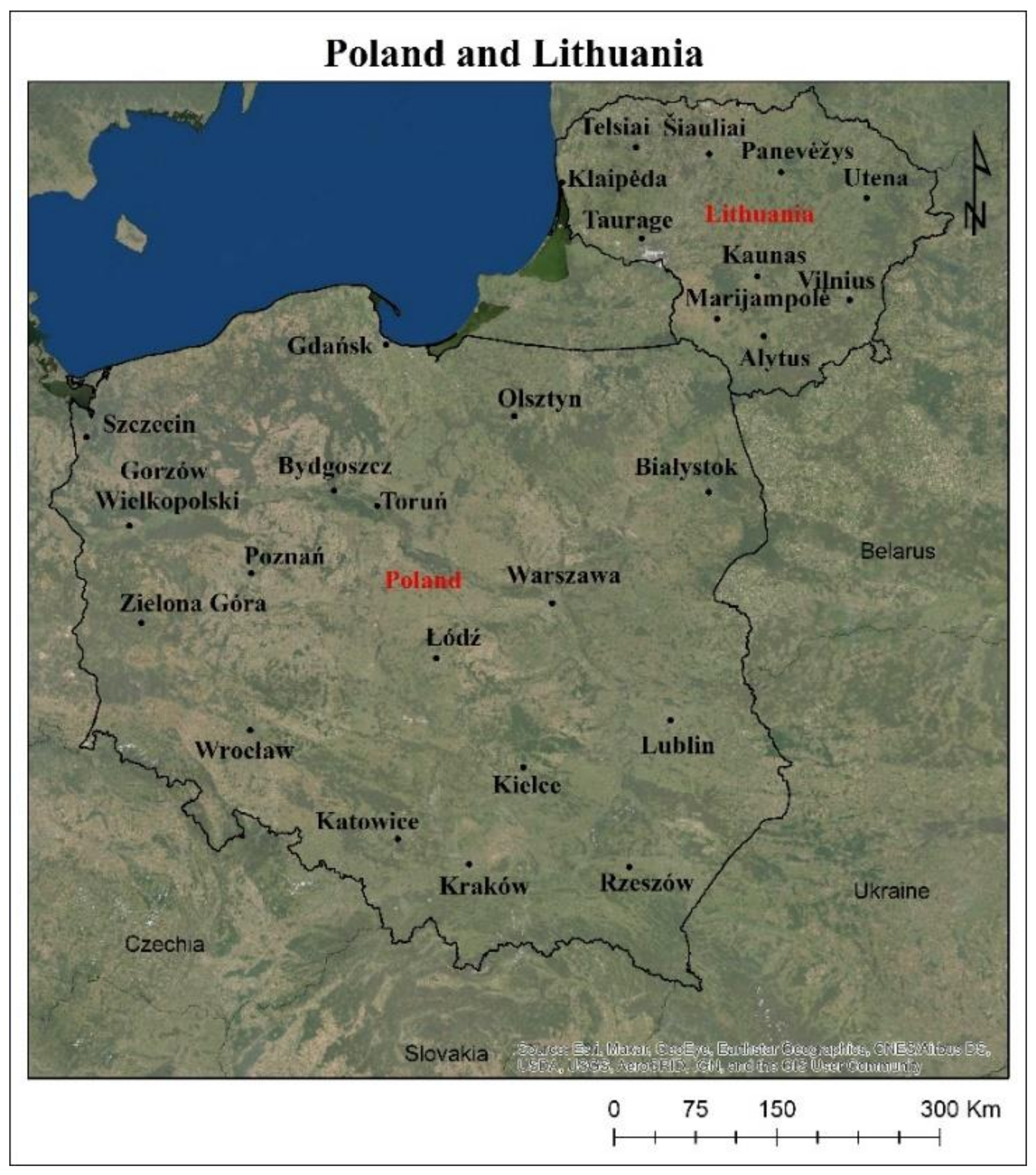
2.1. Study Area

This research focuses on Poland and Lithuania, two neighboring countries located in Central and Eastern Europe (Figure 1) with a long and rich history of commonwealth since the Middle Ages. The economic dynamics of Poland and Lithuania in 2007–2017 were similar, with Poland having been characterized by a more diversified development of regions, while, in Lithuania, development was rather even [36]. This is also emphasized by the GDP (gross domestic product) per capita in Poland, amounting to USD 33,221 and, in Lithuania, USD 37,231 (for 2019), as well as the Human Development Index scores of 0.872 and 0.869, respectively [37]. On the other hand, the two countries differ significantly not only in terms of area, population, and population density (Table 1), but also in the spatial settlement pattern.
Warsaw is the largest Polish city, with a population density of 3412 people/km2. In total, four other Polish cities have more than 500,000 inhabitants, and 16 cities have a population that exceeds 200,000. The most densely populated areas are found mainly in the southern and central parts of the county [39,40], due to significant economic development. In many regions, the population density far exceeds the Polish average, e.g., in the Silesian region, the value is 372 people/km2, which is more than three times the national average [38].
Lithuania is the 17th largest country in Europe. Its capital is Vilnius, and other major cities include Kaunas, Klaipeda, Siauliai, Panevezys, Alytus, and Marijampole. Most Lithuanian cities and towns are small; only six have over 50,000 inhabitants and two have over 200,000, while 65 have fewer than 10,000 inhabitants [41]. Since the 1990s, the country has experienced a constant migration of people from rural areas to cities. The well-planned and executed development of regional centers contributed to this trend.

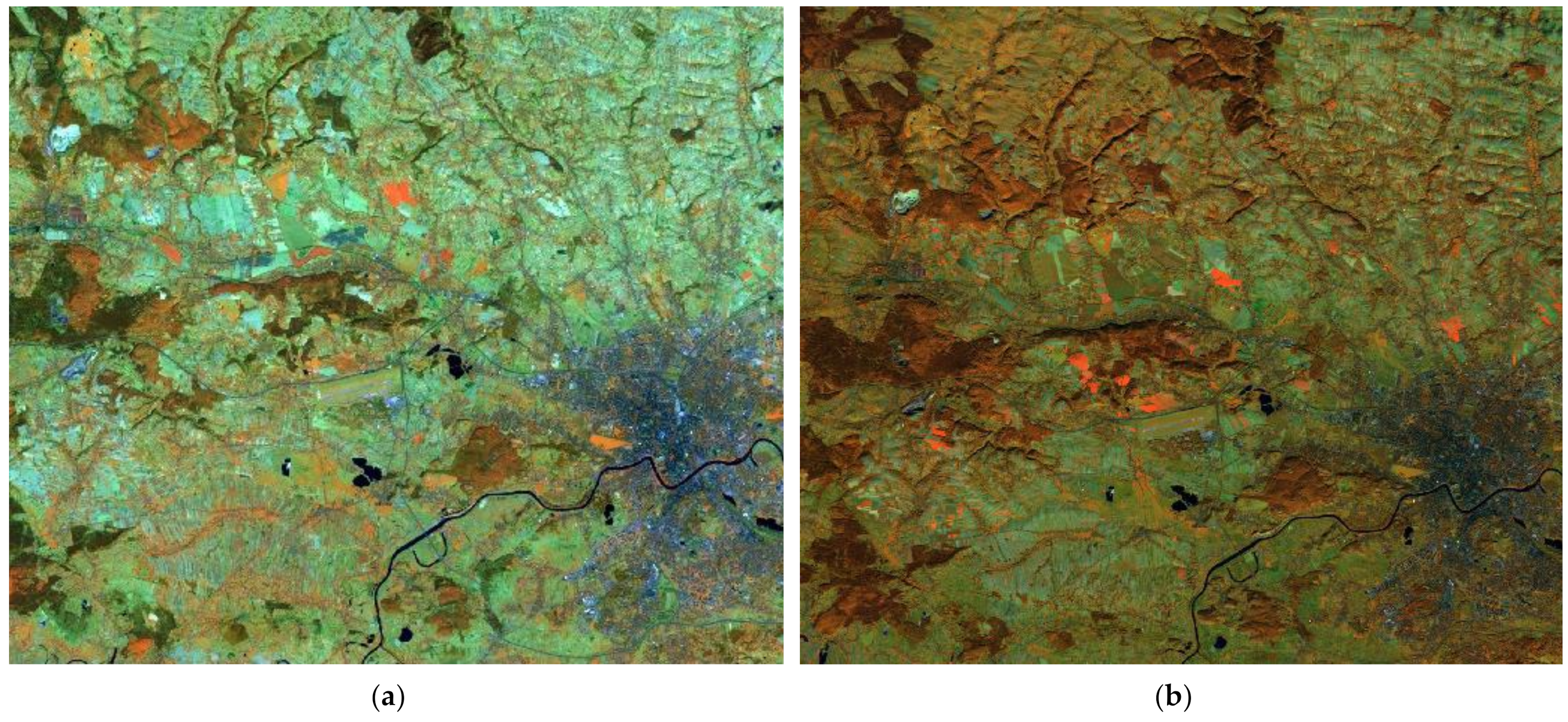
2.2. Data Use Description
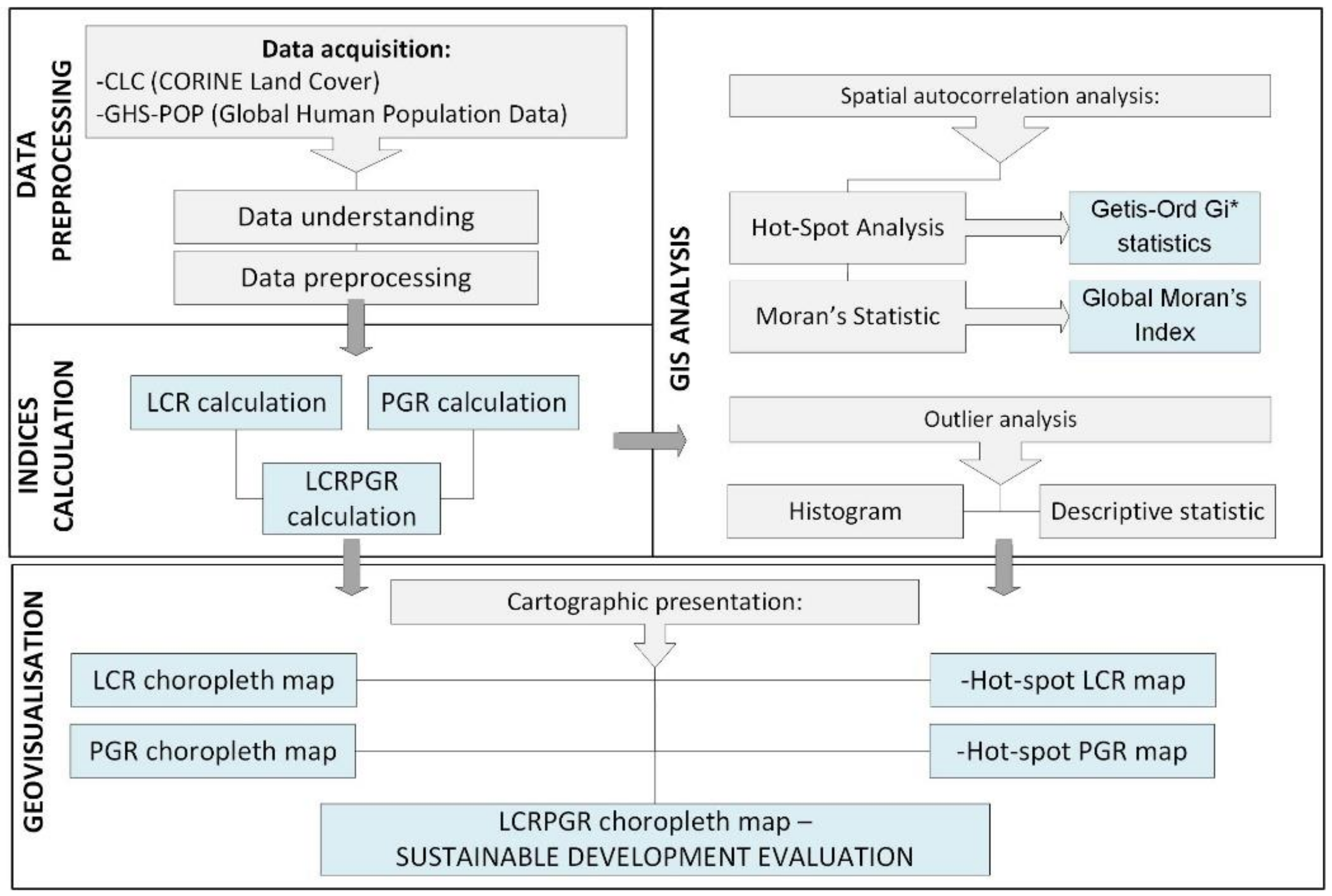
This research used GHS-POP, which consists of open global raster population data provided by the European commission joint research center, presented in an equal-area projection with grids of 1 km by 1 km [42,43,44] (Figure 2). Population estimates for 2000 and 2015 were collected from censuses or administrative units and were assigned to grid cells, employing the disaggregation methodology that uses built-up area data, as described by Freire et al. [42]. The density and distribution of built-up areas are based on satellite images [44,45]. In particular, satellite data from the year 2000 (Landsat-7 ETM+) were acquired from the Global Land Survey (GLS) datasets, pre-processed by the University of Maryland, and described by Gutman et al. [46]. Scenes from the 2015 (Landsat-8 operational land imager (OLI)) collection were downloaded directly from the USGS website [47].
The CORINE land cover (CLC) project was carried out within the European earth monitoring program, the Copernicus Land Monitoring framework. The CLC provides information on the earth’s surface, both physical and biological, including land changed by human construction, agricultural land, woodland, and water bodies [48] based primarily on computer-assisted interpretations of satellite images. Anthropogenic surfaces, agricultural land and woodland, and wetland and water bodies constitute the first level of the CORINE hierarchy, which, in turn, is divided into 15 classes constituting level 2; in comparison, level 3 is made up of 44 classes. Five CLC inventories have been produced for 1990, 2000, 2006, 2012, and 2018. The proposed analysis uses data from 2000 and 2018 (Figure 3).
CLC2000 has been established by the photointerpretation of Landsat-7 ETM images (multispectral and panchromatic), resampled with a 12.5 m resolution, as well as using CLC2018, Sentinel-2A/B, and Landsat-8 [49]. The satellite images are synoptic in nature; therefore, the possibility of the correct classification of the land cover largely depends on the date of image acquisition. Poland was covered by 28 Landsat or IRS images that were delivered due to the atmospheric conditions within a timeframe of three years (four from 1999, 19 from 2000, and five from 2001), which did not facilitate interpretation. Moreover, the acquisition date of satellite images (images from April–May and of late October) hindered the interpretation of built-up areas (see Figure 4).
Artificial areas of level 1 classes have been chosen to represent urban agglomerations. The artificial areas under examination include the following (CLC level 2): urban fabric (continuous and discontinuous); industrial, commercial, and transport units; industrial, commercial, and transport units; mine, dump, and construction sites; green urban areas; and sport and leisure facilities. Ultimately, the mining sites (code CLC 131) were excluded, as they were always outside built-up areas.

2.3. Applied Method

2.3.1. Workflow

Cartographic modelling is based on the assumption that the process of map creation (as well as the spatial database development) is preceded by an understanding the spatial aspects of the reality, including the spatial distributions of objects and phenomena, their mutual interactions, and the processes shaping the geographical space and manifesting themselves with different intensities depending on the considered observation scale [50,51]. Tomlin [52] claimed that cartographic modelling indicates the usage of tools and techniques for analyzing and synthesizing geospatial data by way of a geographic information system (GIS).
The analysis was performed followed cartographic modelling rules, starting from data understanding and processing, the GIS analysis, and the geovisualization of the results in the form of thematic maps (choropleth maps and hotspot maps), as shown in Figure 5. The preparatory stage included data acquisition, their transformation to a common coordinate reference system, and data processing procedures, such as intersecting and compiling statistics that show changes in the number of people and changes in the built-up areas. The preprocessed data were used to determine the land-use effectiveness indicators, namely, LCR, PGR, and LCRPGR. The GIS analysis was based on spatial autocorrelation and consisted of a set of statistics describing how the LCR, PGR, and LCRPGR values were spatially autocorrelated. Moreover, an outlier analysis of the LCRPGR index was performed using a histogram analysis and the associated descriptive statistics. Finally, choropleth and hotspot maps were elaborated to portray the results. ArcGIS pro (2.8.4) and Statistica 13.1 were used to perform the analyses.

2.3.2. LCR, PGR, and LCRPGR Index Calculations

The LCRPGR indicator was calculated as a ratio of LCR-to-PGR [12,53,54,55]. The PGR indicator (Equation (1)) shows the changes in populations for a specific time interval, while the LCR indicator (Equation (2)) reveals the change in development during the same period. Thus, LCRPGR shows the land-use efficiency relative to how much land is used for demographic urban growth. It was calculated for each grid cell in Poland and Lithuania for 2000 and 2018 (Equation (3)):
PGR = ( ln Po p t + n Po p t ) / t
where Popt is the total population for a spatial unit in the initial year, Popt+n is the total population in the final year for a spatial unit, and t is the number of years between the two measurement periods.
LCR = ( ln Ur b t + n Ur b t ) / t
where Urbt is the total built-up area for a spatial unit for the initial year using CORINE land cover data (km2), Urbt+n is the total built-up area for a spatial unit for the final year using CORINE land cover data (km2), and t is the number of years between the initial and final measuring periods.
LCRPGR = LCR PGR
where LCR is the land cover ratio and PGR is the population growth ratio.
The LCR is an indicator of area expansion, while PGR describes the demographic change. The positive values of the former indicate a growing built-up area and the positive values of the latter indicate a growing population. Their values can be negative, indicating a decreasing area or population. LCRPGR can be lower than zero, indicating that either LCR or PGR is negative. Based on the values of the LCR, PGR, and LCRPGR indicators, five classes of land use efficiencies were calculated in Poland and Lithuania (Table 2).
An LCRPGR value close to 1 indicates a significant efficiency of land use, implying a similar value of LCR and PGR. Hence, the rise in built-up areas and the population is proportional. Conversely, areas characterized by inefficient land use are those where, despite an increase in the built-up area, a decline in the population can be observed, in which case LCRPGR assumes values below −1. The analysis of the outliers of LCRPGR required the determination of descriptive statistics. It was assumed that outliers occur when the index values exceed 2.0 standard deviation values (SD) from the mean [56]. Choropleth map classes were selected to increase the effectiveness of the cartographic communication; negative values of indicators related to the decrease in the built-up area are in a blue hue, while the increase in the built-up area is presented in a red hue.

2.3.3. Spatial Autocorrelation

The scientific literature describes a few possible techniques of spatial pattern analyses [57,58,59]. The hotspot analysis creates groupings of similar values within a given area, where low values clusters represent cold spots, and high values represent hotspots. Formulas (4) and (5) were used for the hotspot analysis (Getis-Ord Gi*) [60,61]:
G i * = j = 1 n w i , j w j X ¯ j = 1 n w i , j   S [ n j = 1 n w i , j 2 ( i , j n w i , j ) 2 ] n 1
where xj is the value for the feature j attribute, wi,j is the spatial weight between feature i and j, n equals the total number of features, and
X ¯ = j = 1 n x j   n   S = j = 1 n x j 2   n X ¯ 2
A statistically significant hotspot is defined by an area with a high value that is also surrounded by areas with high values. The local aggregate for a spot and its surroundings is compared to the proportional aggregate for all spots. When these two values differ significantly, the deviation should be verified to ensure that this difference is not the result of a random occurrence. If this is not the case, a statistically significant z score is obtained [62].
The Global Moran’s I index, calculated according to Formula (8), was used to investigate spatial autocorrelation [63].
I = n i = 1 n j = 1 n w i , j y i y ¯ y j y ¯ n i = 1 n j n w i , j y i y ¯ 2
where n is the total number of features, y is the value for a feature, y ¯ is the mean of y, and wi,j is the spatial weight between feature i and j. The Global Moran’s I index value should range between −1, indicating spatial dispersion, and +1, indicating spatial clustering. Spatial clustering means that features with the same characteristics are close to one another. When they are located away from one another, they are spatially dispersed. A Moran’s I value of 0 means that the features are randomly distributed [64].

3. Results

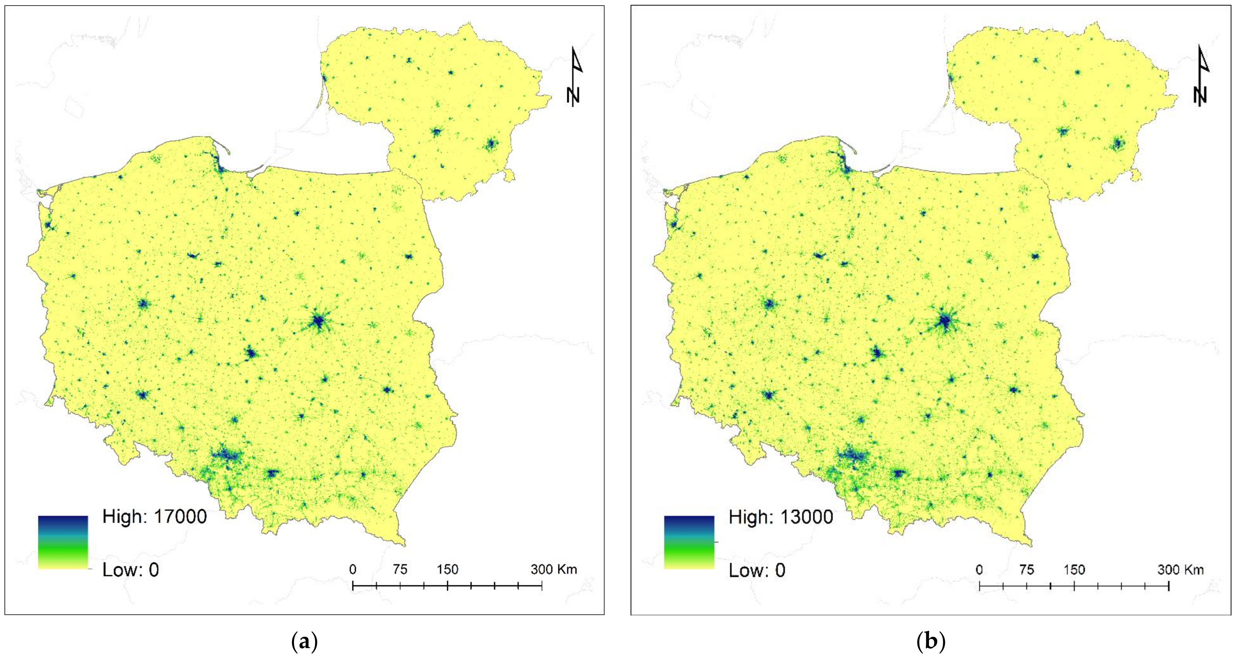
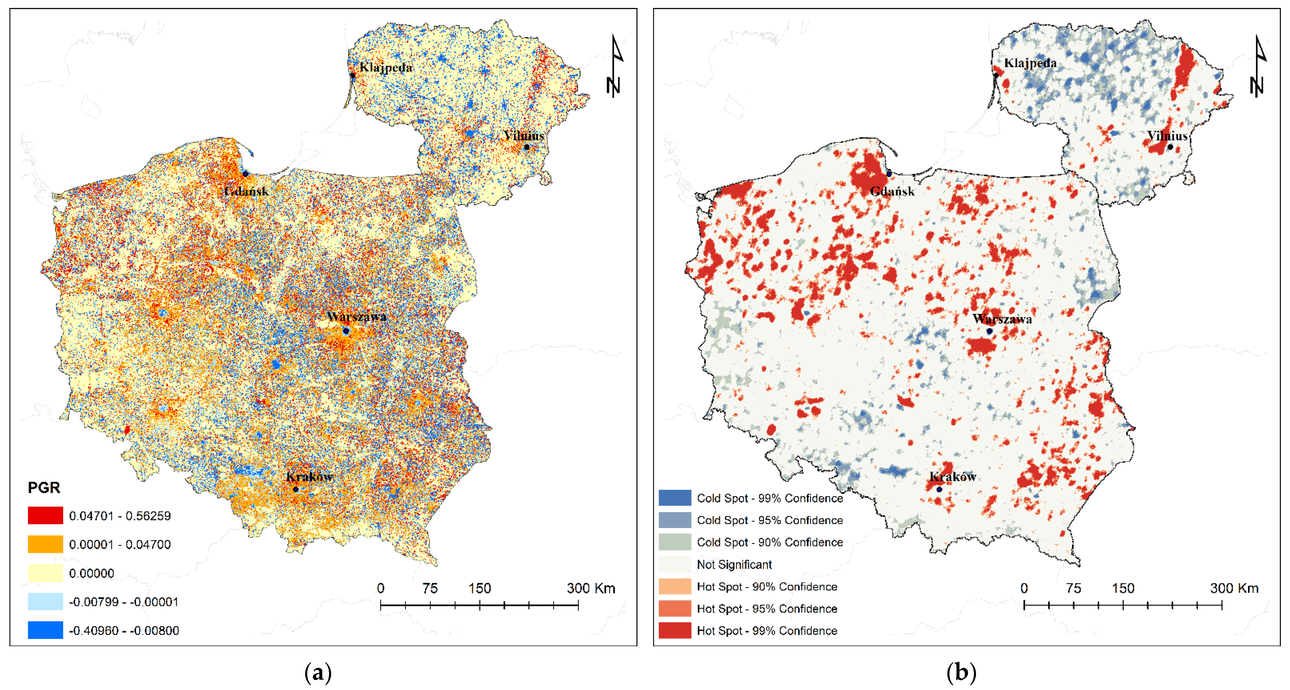
3.1. Population Growth Rate

The PGR index used to quantify the demographic change between 2000 and 2015 (Figure 6a) assumed negative values in big Polish and Lithuanian cities. The average PGR, in Poland, was 0.01323, and in Lithuania it was 0.00675. In Poland, the lowest PGR value, −0.40960, was observed in Wrocław, and the highest value, 0.55720, was observed in Rzeszów. The population of large 16 provincial cities of Poland significantly decreased between 2000 and 2015. An important population decline was observed in the south of the country, especially in urban agglomerations, the center of which is Katowice. The lowest PGR value in Lithuania was perceived in Siauliai city, −0.09323, and the highest value, 0.56259, was in the suburbs of Vilnius (Figure 6a). In large and medium cities, with a population of more than 100,000 inhabitants, a decline in the population number between 2000 and 2018 was observed. The results of the hotspot analysis (Figure 6b) showed some groupings of high and low index values in the northern part of Poland, including Gdansk vicinity, Bydgoszcz, Toruń, and Olsztyn, as well as other parts of the country, such as areas around Warsaw, Rzeszów, and Lublin. In Lithuania, the hotspot areas of concentration were observed outside the center of Vilnius, Utena, and Klaipeda. On the other hand, cold spots were detected throughout northern Lithuania and southern Poland, near Katowice.
In Poland, the number of grid cells with a PGR index equal to zero amounted to 137,633 (43.9%), while population growth with a PGR > 0 was observed for 104,382 grids (33.3%). These statistics slightly differed in Lithuania, with a stable population observed for 46,495 grids (70.7%) and population growth for 8313 grids (12.6%). Significantly higher negative PGR data were observed in Poland (almost 10 times higher). The PGR histograms for Poland and Lithuania have right-skewed distributions, with skewness values of 3.05769 and 3.05769, respectively, as well as a mean of 0.013229 (Poland) and 0.006748 (Lithuania) and a median of 0.000 for both countries. Furthermore, for 50% of the grids, the PGR index fluctuates from 0.000 to 0.009 (lower and upper quartile) in Poland and from −0.014 to 0.015 (lower and upper quartile) in Lithuania.

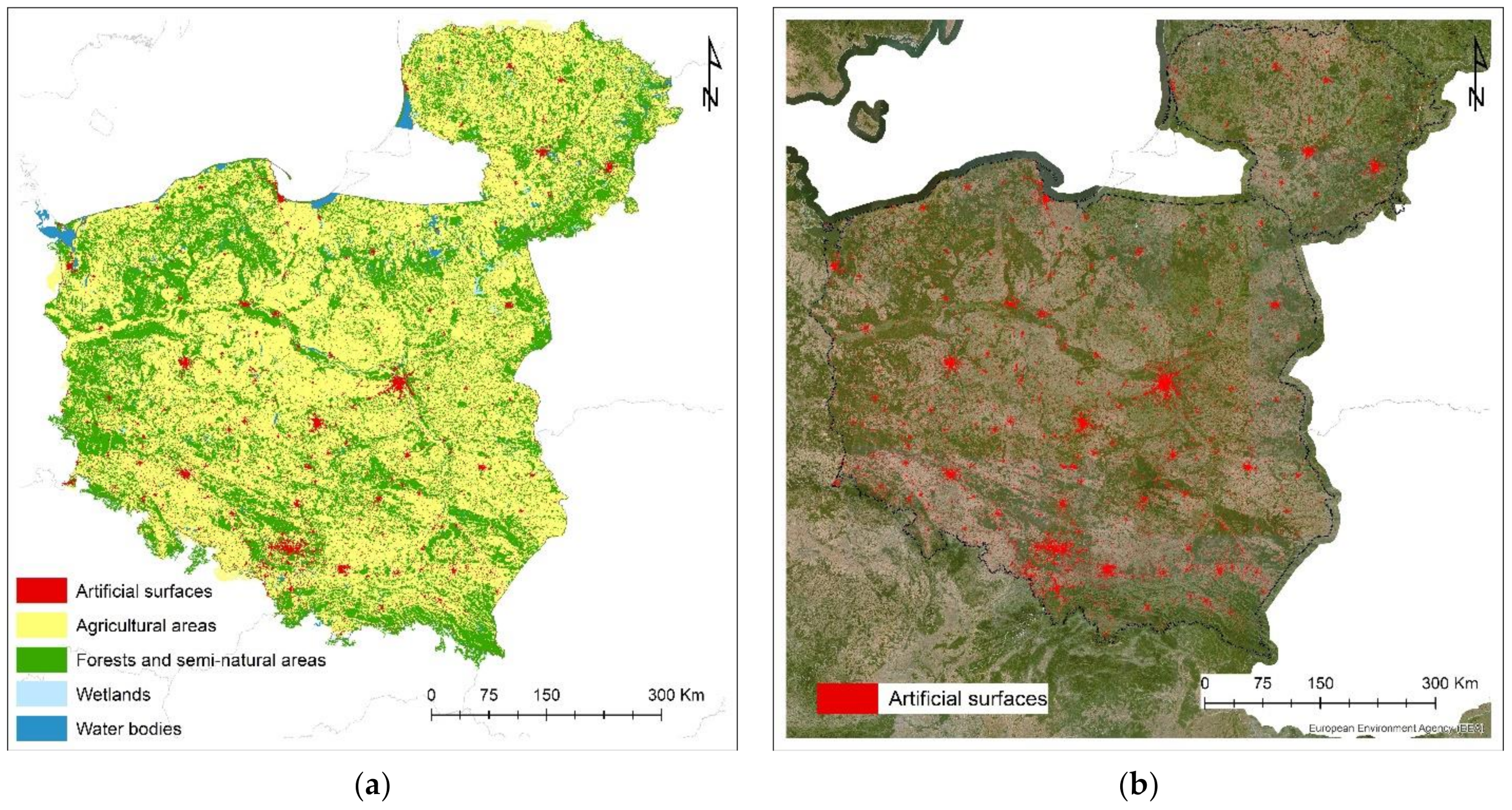
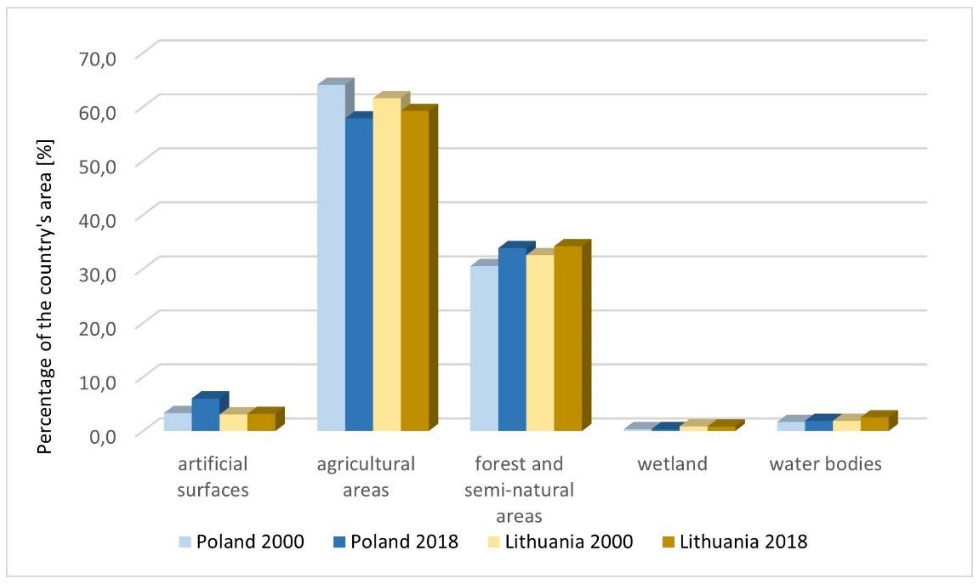
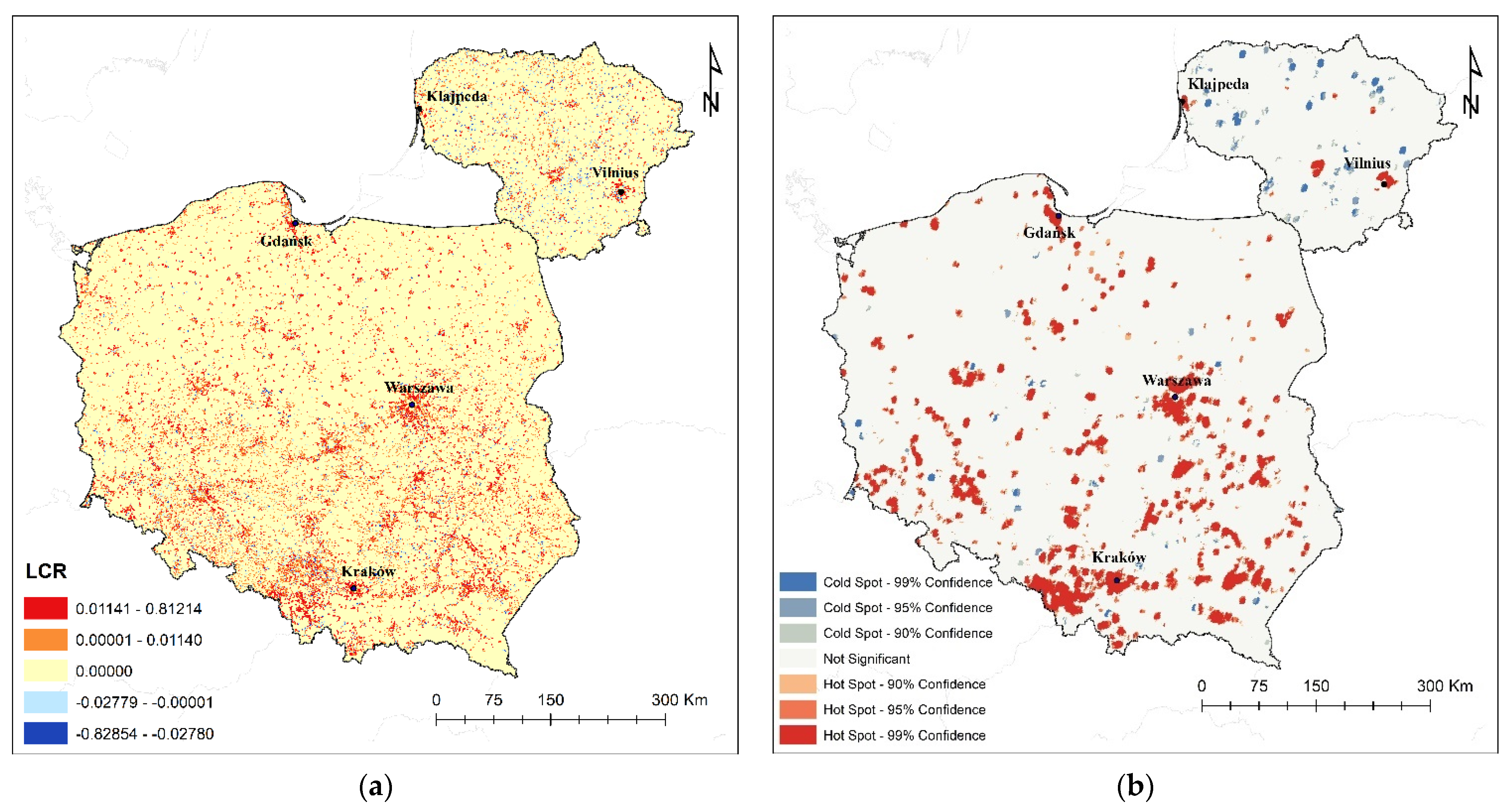
3.2. Land Cover Ratio

The analysis of land cover in Poland and Lithuania showed that the agricultural areas decreased, and that there is a noticeable expansion of built-up areas (Figure 7). The artificial surfaces in Poland increased from 3.3% to 6.6%, and agricultural land decreased from 64.1% to 57.9%. In Lithuania, the built-up areas increased slightly, from 3.1% to 3.2%, and the agricultural areas decreased (from 61.6% to 59.2%). These results show urban expansion into rural areas, which is associated with taking over agricultural land for single-family and multi-family housing.
The LCR index presents the land consumption rate in 2000 and 2018 (Figure 8a). The lowest LCR value, −0.81214, was observed in Poland, near Warsaw, while the lowest value of the index in Lithuania was −0.70950 and occurred near the city of Telsiai. The highest value of the index in Poland was 0.81214, whereas for Lithuania, it was 0.6664. Most of the areas with negative development growth in Poland are located around Katowice, where the reclamation of mining and the associated devastation of areas were taking place. The LCR grew from the center to the outskirts in big cities, such as in Kraków or Warsaw. The LCR value formed hotspots of high values (Figure 8b) in the vicinity of large cities, such as Warsaw, Kraków, and Kielce in Poland. In Lithuania, hotspots were identified around Klaipeda and Vilnius.
The average LCR was 0.046229 in Poland and 0.006748 in Lithuania, indicating urban expansion between 2000 and 2018. In Poland, the LCR was more diverse, with a variance of 0.014643, whereas in Lithuania, this statistic amounted to 0.00035. The LCR value histograms indicate that the index distribution is close to normal, with a skewness coefficient of −0.325 in Poland, and −1.4335 in Lithuania.
The simple linear regression coefficient between the LCR and PGR, in Poland, equaled 0.03, and in Lithuania, it equaled 0.02 (with p < 0.0500). The low coefficient value indicates that the relationship between the LCR and PGR was very weak.
The Global Moran’s I statistics of the LCR and PGR values returned positive I and z-score values for both Poland and Lithuania, with a 99% level of significance (Table 3). Therefore, it is possible to reject the null hypothesis that the values of indicators are randomly distributed within the area of the two countries. Hence, it was assumed that the indicator values are clustered in the whole study area.

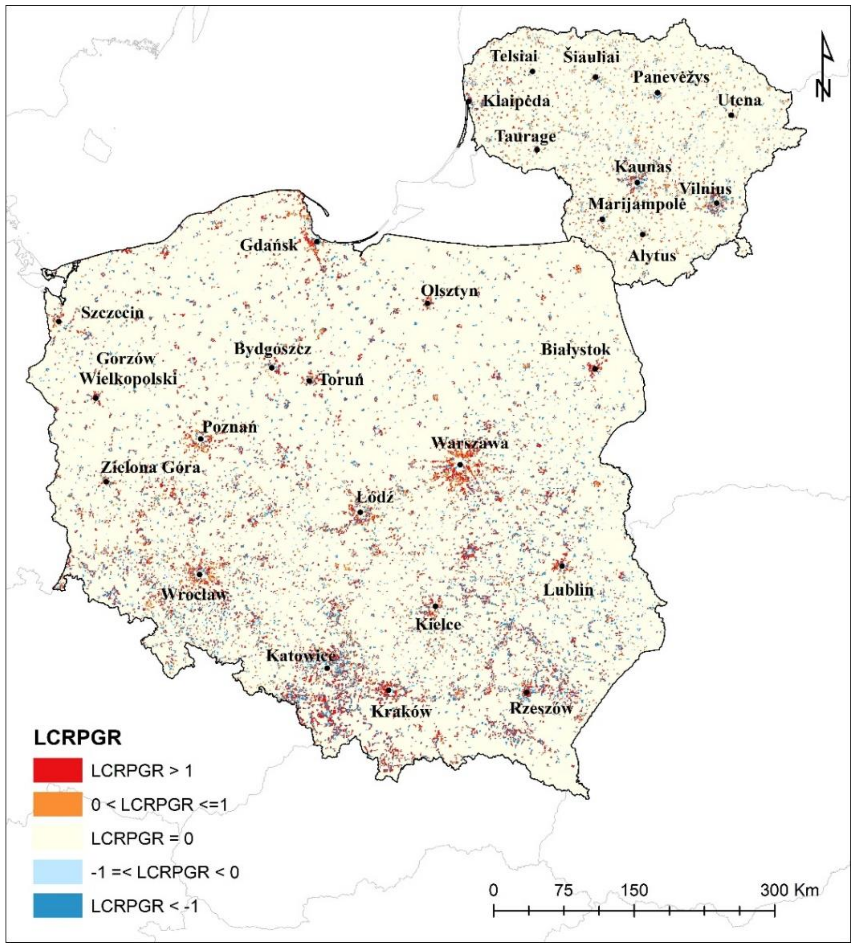
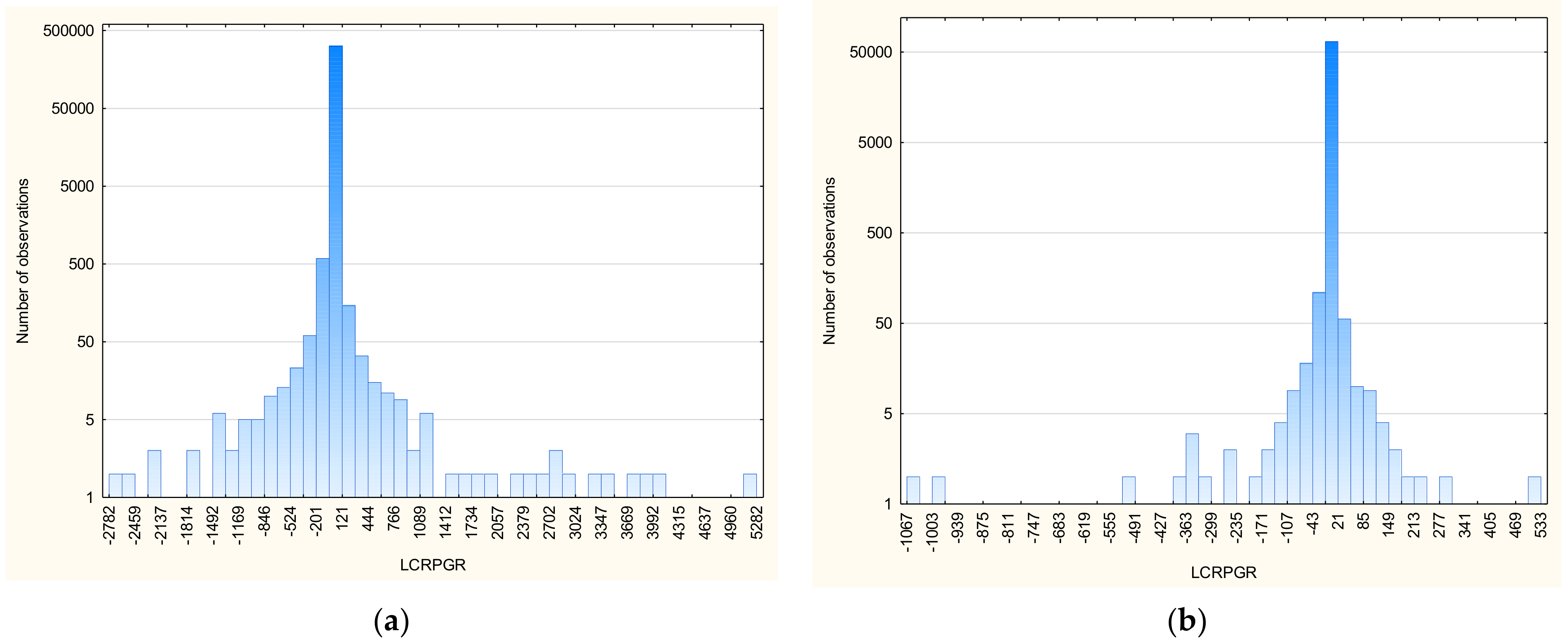
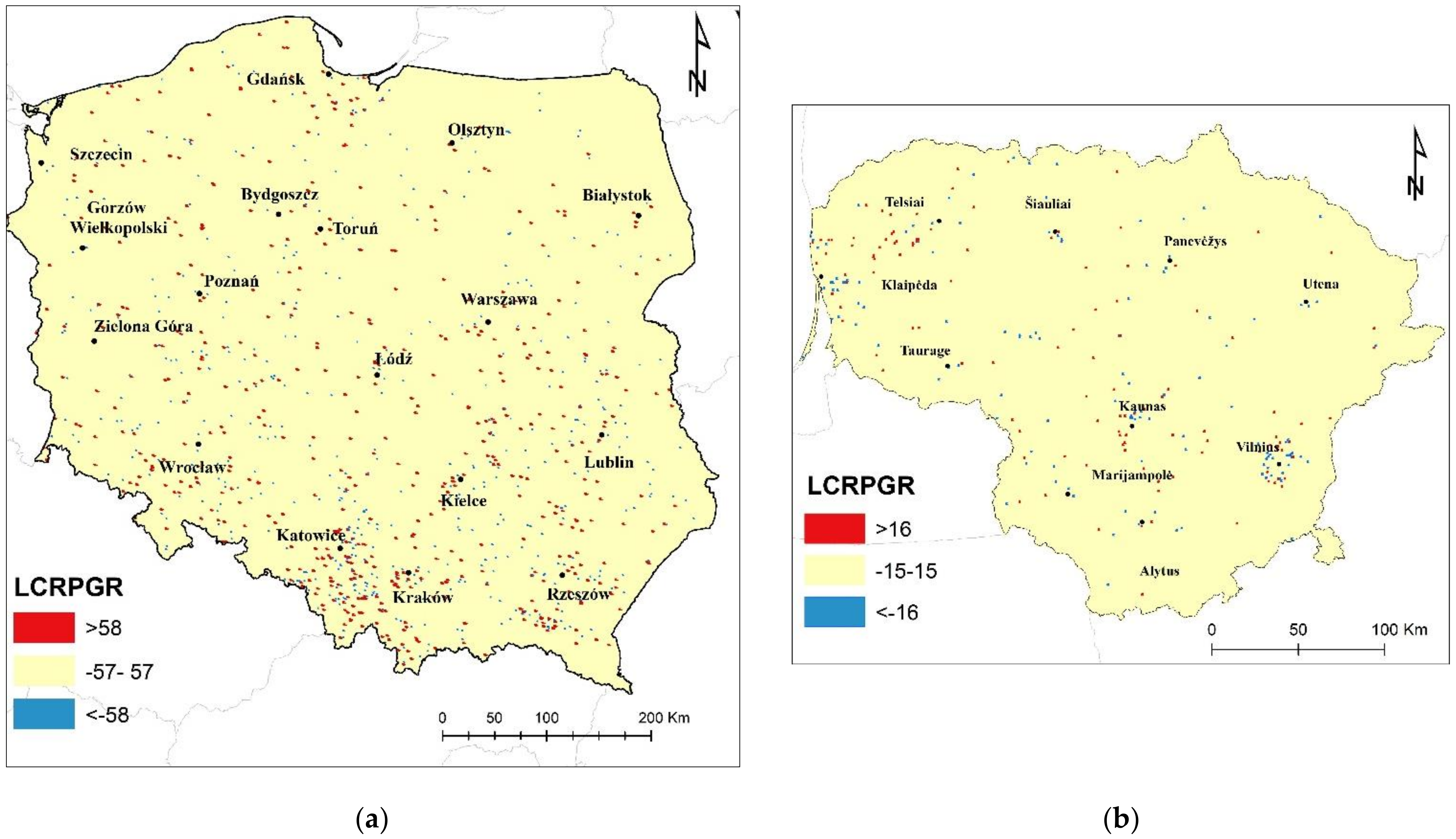
3.3. LCRPGR Visualization and Analysis

The cartographic presentation of the LCRPGR index, shown in Figure 9, made it possible to identify areas where the population growth was balanced with the increase in built-up areas (0 < LCRPGR < = 1), but also where the rate of urban area expansion was greater than the demographic growth (LCRPGR > 1), or places where demographic decline was simultaneous with spatial expansion (LCRPGR < 0).
The analysis of the LCRPGR values shows that 26.4% of built-up areas in Poland and 22.9% of built-up areas in Lithuania were areas with the sustainable development of urbanization and population, while 15.5% of Poland and 29.8% of Lithuania were characterized by a LCRPGR equal to zero. These were mainly areas with no changes, in the centers of big cities. Almost 24.8% of built-up areas in Poland and 28.1% of built-up areas in Lithuania were areas where the LCRPGR value was between −1 and 0. These were areas with an increase in urbanized areas and a decrease in population or a decrease in urbanized areas with an increase in population, where the absolute values of the LCR and PGR are similar. These areas were labelled as moving away from efficiency. In Poland and Lithuania, there were mainly areas with a LCR > 0 and a PGR < 0 that covered 16.1% and 21.9% of built-up areas, respectively.
According to Table 1, areas with LCRPGR > 1 in Poland covered 17.9%, of which the vast majority, i.e., 15.3%, were characterized by PGR and LCR values above 0, indicating a disproportionately large increase in urban development in relation to the increase in population. In Lithuania, 11.6% of built-up areas were characterized by LCRPGR values greater than 1, but the vast majority, i.e., 8.5%, were areas with LCR < 0 and PGR < 0. They were characterized by a disproportionate decrease in built-up areas in relation to the decrease in population. Areas with insufficient land use, for which LCRPGR values were less than −1, occupied 15.4% of the built-up territory of Poland, while in Lithuania they were halved, and covered only 8.5% of the build-up area.
The average LCRPGR value in Poland was 0.115, and in Lithuania, it was −0.054. The variance of the index in Poland was 855, which indicated a great range; in Lithuania, the variance was 64. The standard deviations were 29 for Poland and 8 for Lithuania. The histogram of the LCRPGR in Poland was right-skewed, with a skewness coefficient of 57.32, while, in Lithuania, the skewness was −69.35 (it was a left-skewed distribution). In total, 44.3% of built-up areas in Poland and 34.6% of built-up areas in Lithuania were characterized by positive values of the index (Figure 10).
A histogram analysis of the LCRPGR index confirmed the existence of outliers. The analysis, based on the standard deviation of the index and the mean, showed that, in Poland, the index outliers were below −58 and above 58. This means that 518 grids took negative values (marked in blue), while 541 took positive values, marked in red (Figure 11a). In Lithuania, the LCRPGR outlier values were below −16 and above 16. For 121 grids, the values were negative, and for 114 grids, the values were positive (Figure 11b).
The LCRPGR outliers in Poland and Lithuania were caused, inter alia, by errors in the interpretation of the built-up areas in satellite images from the year 2000 and 2018, as shown in Figure 12 and Figure 13.
Undoubtedly, the occurrence of the LCRPGR outliers was also influenced by the reliability of the GHS-POP data. The GHS-POP represents the so-called “resident-based population”, which denotes the residential population allocated to built-up areas. However, such an assumption could result in assigning people also to non-residential areas and, ultimately, could lead to a distortion of the number of people assigned to the grid cells (Figure 14). As a result, the PGR assumed erroneous values and resulted in LCRPGR outliers.

4. Discussion

4.1. Brief Comparative Analysis between Poland and Lithuania

Comparing the results of the analyses in Poland and Lithuania, we observed both similarities and significant discrepancies. From 2000 to 2018, depopulation in Lithuania amounted to 0.67%, a value twice as low as that in Poland (1.32%). As shown in Table 2, it was caused by a decrease in births and an increase in migration. The spatial pattern of highly depopulated regions also differed; in Poland, the population decline was mainly concentrated in the provincial city centers and the Katowice metropolitan area. In Lithuania, depopulation covered the whole country, except the Vilnius–Utena belt.
In Poland, from 2000 to 2018, the built-up area doubled (with an upsurge from 3.3% to 6.6%), while in Lithuania, it remained basically the same (3.1% of the country’s area in 2000 and 3.2% in 2018). A consequence of the urban area expansion was a positive value of the land consumption indicator. The annual growth of LCR in the analyzed period in Lithuania was almost seven times lower than in Poland and amounted to 0.67% and 4.62%, respectively. This was perfectly highlighted by the hotspot map (Figure 8b).
The highest divergence was visible when analyzing LCRPGR, the final land use efficiency indicator. In Lithuania, this indicator equaled −0.054, which, in light of the LCR and PGR, indicated nearly balanced changes in the population and in built-up areas. On the contrary, in Poland, the LCRPGR was 0.115, indicating growth in built-up areas at a higher rate than population change.
To summarize, the synthesis of spatiotemporal territorial trajectories was as follows. The LCR pattern illustrated an increase in the index values from the center to the periphery in large cities, while the PRG typified a decrease in the values from the center to the city fringe. Ultimately, the spatiotemporal trend of the LCRPGR in the 2000–2018 period was characterized by a decrease in the index value from the center of urban areas, where it is above 1, towards the outskirts, with negative values of the indicator.

4.2. Concise References to LCRPGR Studies

There are many articles in the literature on LCRPGR monitoring at global [18,35], national [21], or local [19,65] levels. As underlined by Nicolau et al. [21], 2018, the procedures adopted for assessing SDG 11.3. 1 diverge from country to country. Therefore, comparing the results is very difficult and is only indicative.
Considerable worldwide variations in the LCRPGR over the period of 1990–2015 were noted by Schiavina et al. [18] as well as Melchiorri et al. [35]. Based on GHSL and GHS-POP, they found that, in Europe, the index had an average value of 20.2 between 1990 and 2000, and then dropped to 7.8 in the 2000–2015 period. The above-mentioned global studies showed that Poland, like most European countries in the 1990–2015 epoch, was characterized by a SDG 11.3. 1 index greater than 2, which meant that the land consumption rate more than doubled that of the population growth. On the other hand, Lithuania was assigned an LCRPGR in the range of 0 to −1, which indicated moving away from efficiency. The results of the evaluation of SDG 11.3. 1 in Poland and Lithuania, presented in this paper, are in line with the global national-level analysis, presenting the values of the indicator in the same ranges for both countries. Similar conclusions were drawn based on our research conducted in Poland; however, it was at a much more detailed level.
National-level research conducted by Nicolau et al. [21] showed that most Portuguese municipalities in 2007–2011 and 2011–2015 had negative LCRPGR values. This indicated that human-made surfaces grew, while the population decreased. These results are very similar to the results presented in this study for Lithuania, and they differ from the results obtained in Poland.
Ghazaryan [65] also made similar observations estimating the LCRPGR in North Rhine-Westphalia. The authors found that the land-use change, and population growth do not always run in parallel. The following results led to these conclusions. In the years 1985–2005, the indicator was positive in most municipalities, while in 2005–2017, some of them were characterized by negative LCRPGR values, which indicated an increase in land consumption relative to urban population reduction.
The above studies showed variations in the land-use efficiency in Europe and around the world, but did not explain their causes; they only advocated the environmental, economic, and social discrepancies.

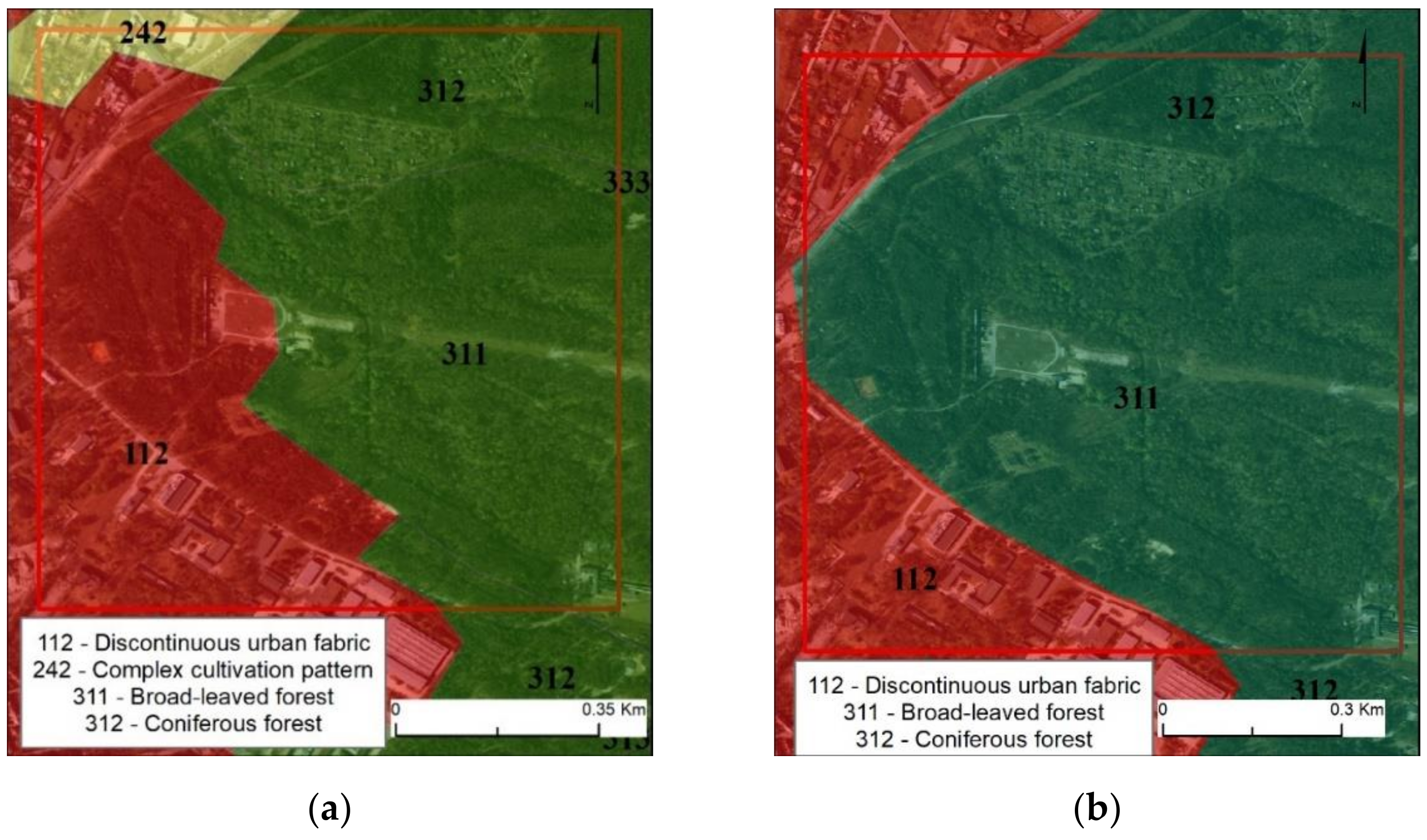
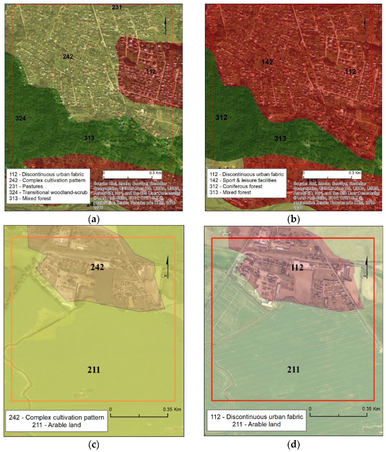
4.3. Semantic Uncertainty

When calculating the SDG 11.3. 1 indicator, attention should be paid to the semantic uncertainty in the definitions of the used data. It is important to note that there is some confusion in the definition of the ’built-up areas’ used in the calculation of the LCR indicator. Seeing as a consensus on the definition of the indicator 11.3. 1 has not yet been agreed upon, some confusion still exists regarding the land type which it addresses [20,66,67]. Song et al. [67] defined a built-up area as the core of the city, while eliminating the rural terrains on the periphery, which was implemented by Wang et al. [20]. Nicolau et al. [21] used the artificial areas of the CORINE land cover data, excluding construction sites, when calculating the indicators for Portugal. The analysis of CLC data showed that the built-up areas were generally properly distinguished when the generalization guidelines were followed [68]. “The thematic accuracy of the CORINE land cover 2000” report [49] pointed out that the “urban fabric” class reliability is over 95%. However, some errors were observed, mainly commissions and omissions, which amounted to 42% and 43% of all errors, respectively [35]. In total, 12% of all errors resulted from incorrect generalizations, and 2% of all errors were from the inaccurate delineation of CLC classes (if the positional error exceeds 100 m).
The indicators calculated for the United Kingdom use the term human-made surfaces, while, in France, the urban area refers to artificial areas [66]. It is worth mentioning that semantic uncertainty is not only a drawback of the CLC datasets, but also of open and freely available land use/land cover datasets used all over the world. Congalton [69] noted that there are many semantic uncertainties in the definitions of land use classes and, especially, the mixed classes were the most ambiguous.
Given that Goal 11.3 is to, “by 2030, enhance inclusive and sustainable urbanization and capacity for participatory, integrated, and sustainable human settlement planning and management in all countries” [18,21], we established that the land type addressed by the indicator is urban land comprising of both the built-up areas and the open urban spaces. Hence, the CORINE land cover classes chosen to represent built-up areas were the artificial areas. Urban development often takes place at the expense of other types of non-urban land (e.g., agricultural and forest land); therefore, it is important not to limit the analyses to the administrative boundaries of the city.
Melchiorri et al. [35] and Freire et al. [42] proved the validity of utilizing the GHSL to estimate the LCRPGR. Additionally, it is worth emphasizing that the GHSL is produced from open-source data with the capacity for the multitemporal mapping of the dynamics of built-up areas (Landsat imagery and the Gridded Population of the World, version 4) [35,70,71]. The high accuracy of those data was also proved by Calka et al. [46], although the GHS-POP tends to underestimate the population in densely built-up areas and to overestimate the population in transitional areas (the areas between urban and rural). At the national level, MAPE ranges from 1.5% to 1.6% for the 250 m and 1 km resolutions of GHS-POP data in Poland. At the local level, however, the error rates range from 4.5% to 5.8%. Archila-Bustos [72] pointed out that the great advantage of GHS-POP is that it limits the population to built-up zones; hence, population density is proportional to the built-up area density.
Uncertainty is an inherent attribute of every spatial data set and, as Bielecka and Burek [73] stated during an in-depth review analysis of the quality and uncertainty of spatial data, and each data user is aware of it. The articles on SDG 11.3. 1 monitoring that have been published so far do not address the problem of outliers, as they provide the values of the indicator in predetermined ranges, which, of course, does not mean that there are no outliers (gross errors). Demonstrating that data and spatial analyses are not error-free is a valuable part of our research study, as it makes future readers aware of this fact. Moreover, and most importantly, it highlights that outliers, in general, constitute a small fraction of all values. In the presented research study, they account for 0.34% of all values in Poland and 0.38% of all values in Lithuania. Moreover, the outstanding values are randomly distributed throughout the country. This, in no way, limits the validity of the final results.

4.4. Land Use Efficiency Interpretation Problems

Because of the methodology used to assess SDG 11.3. 1, this indicator can lead to undefined values, where the PGR is 0. It is not possible to calculate the indicator when the population has not changed in the examined period. In built-up areas, the population dynamics are so high that the number of people changes (decreases or increases) constantly. The interpretation of the LCRPGR (land use efficiency) can also be ambiguous when we do not have any information about the land use changes and population growth. Negative LCRPGR values may indicate two opposite scenarios: population growth and a land use decrease or, inversely, a population decrease and a land use increase. Nicolau et al. [21] and Corbane et al. [70] also pointed out the difficulties in interpreting the LCRPGR. Similarly, when the LCRPGR reaches positive values, it can correspond to two situations: an increase in the population and an increase in the land consumption or, inversely, a decrease in the population and a decrease in the land consumption. Therefore, many researchers present the values of the changes in built-up areas and the population as a percentage.

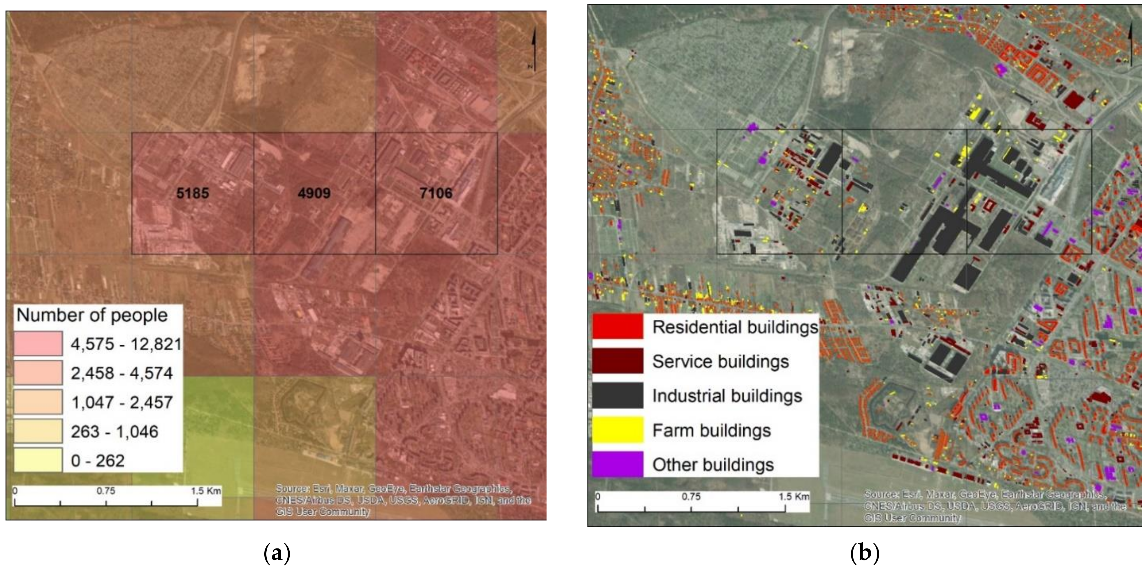
4.5. Cartographic Presentation Challenges

Choropleth maps, using a pixel-based analysis of the quantitative SDG 11.3. 1 results, were chosen to show a more detailed spatial distribution of the indicators to understand the spatial variability of resource distribution. In particular, we proposed a cartographic modelling process based on GIS analyses, including hotspot and autocorrelation analyses. An important stage was the selection of a proper color scale and cartogram class, so as to increase the effectiveness of the cartographic presentation of the maps. The applied process of qualitative map generalization, based on quantitative grouping, makes it possible to increase the legibility of the resulting maps, which can be a valuable tool in analyzing sustainable development goals. A similar observation was also made by Cybulski et al. [74] while analyzing landscape changes in industrial areas.

5. Conclusions

Thanks to the technological developments in mapping human settlements and the availability of open data, such as CORINE land cover or GHS-POP, it is possible to calculate the land-use efficiency with the use of a pixel-based analysis. This paper confirmed that an assessment of the SDG indicator 11.3. 1, based on earth observation data, could improve the information deficit concerning the land-use efficiency on a fine scale. The methodology presented is universal and can be applied in any country or region, as it is based on the UN’s recommendation for the ratio of the land consumption rate to the population rate, and uses open remotely sensed data.
A significant spatial expansion of built-up areas was observed, especially in Poland. Our research study shows that, between 2000 and 2018, the spatial expansion of build-up areas consumed, in Poland, 8.891 km2 and, in Lithuania, 178 km2. Those areas are mainly located outside big cities in both countries. An important trend is the movement of the population from the center of big cities to the outskirts, or the adjacent areas of these cities. The LCRPGR values in Poland are much higher than those in Lithuania. This is caused by a big differentiation between the values of the built-up area changes and the population growth rate. Moreover, the analysis of the LCRPGR results, at the pixel level, including the evaluation of the sources of error and uncertainty, is prudent and enlightening.
The results of cartographic modelling are gathered on thematic maps, which are an effective and easy-to-use tool to present the land use efficiency in Poland and Lithuania and may be useful in monitoring the sustainable development goals.
Our further research projects will be focused on applying the elaborated methodology to estimate the SDG 11.3. 1 values in European capital cities.

Supplementary Materials

The following are available online at https://www.mdpi.com/article/10.3390/rs14051074/s1, Table S1: Settlement area and population datasets used in land efficiency modelling, ordered by scale.

Author Contributions

Conceptualization, B.C.; methodology, B.C.; software, B.C.; formal analysis, B.C.; resources, B.C., S.M.; data curation, B.C.; writing—original draft preparation B.C., A.O., S.M., E.B.; writing—review and editing, B.C., A.O., E.B.; English correction–A.O.; visualization, B.C.; supervision, E.B.; funding acquisition, B.C., A.O. All authors have read and agreed to the published version of the manuscript.

Funding

This research and publication process was funded by the Military University of Technology, Faculty of Civil Engineering and Geodesy, grant number 531-4000-22-785/UGB/2022.

Data Availability Statement

GHS-POP grids were produced in the frame of the Global Human Settlement Layer (GHSL) project by the European Commission, Joint Research Centre, in Ispra, Italy and were gained from https://ghsl.jrc.ec.europa.eu/ghs_pop.php on 10 January 2021. Corine Land Cover data were obtained from the COPERNICUS Land Monitoring Service web page https://land.copernicus.eu/pan-european/corine-land-cover on 20 January 2021. Boundaries of NUT0 were gained from the Eurostat GISCO Database web page https://ec.europa.eu/eurostat/web/gisco/geodata/reference-data/administrative-units-statistical-units/nuts on 22 October 2021. All satellite imagery was acquired from the Esri Basemaps open source ArcGIS Platform.

Acknowledgments

The research was conducted during Beata Calka study visit at the Vilnius Gediminas Technical University–Vilnius Tech, under the Erasmus + Program (2021).

Conflicts of Interest

Authors declare no conflict of interest. The funders had no role in the design of the study; in the collection, analyses or interpretation of data, in the writing of the manuscript, or in the decision to publish the results.

References

  1. Scott, J.; Marshall, G. A Dictionary of Sociology; Oxford University Press: Oxford, UK, 2009; ISBN 978-0-19-953300-8. [Google Scholar]
  2. Berg, L.; European Coordination Centre for Research and Documentation in Social Sciences. Urban Europe, a Study of Growth and Decline; Pergamon Press: Oxford, NY, USA, 1982. [Google Scholar]
  3. Champion, T. Urbanization, Suburbanization, Counterurbanization and Reurbanization. In Handbook of Urban Studies; SAGE Publications Ltd.: London, UK, 2001; pp. 143–161. ISBN 978-0-8039-7695-5. [Google Scholar]
  4. Schmid, C.; Karaman, O.; Hanakata, N.C.; Kallenberger, P.; Kockelkorn, A.; Sawyer, L.; Streule, M.; Wong, K.P. Towards a New Vocabulary of Urbanisation Processes: A Comparative Approach. Urban Stud. 2018, 55, 19–52. [Google Scholar] [CrossRef]
  5. Dieleman, F.; Wegener, M. Compact City and Urban Sprawl. Built. Environ. 2004, 30, 308–323. [Google Scholar] [CrossRef] [Green Version]
  6. Wegener, M.; Fuerst, F. Land-Use Transport Interaction: State of the Art. 2004. Available online: http://dx.doi.org/10.2139/ssrn.1434678 (accessed on 20 September 2021).
  7. Kocur-Bera, K.; Pszenny, A. Conversion of Agricultural Land for Urbanization Purposes: A Case Study of the Suburbs of the Capital of Warmia and Mazury, Poland. Remote Sens. 2020, 12, 2325. [Google Scholar] [CrossRef]
  8. Liu, J.; Kuang, W.; Zhang, Z.; Xu, X.; Qin, Y.; Ning, J.; Zhou, W.; Zhang, S.; Li, R.; Yan, C.; et al. Spatiotemporal Characteristics, Patterns, and Causes of Land-Use Changes in China since the Late 1980s. J. Geogr. Sci. 2014, 24, 195–210. [Google Scholar] [CrossRef]
  9. Mudau, N.; Mwaniki, D.; Tsoeleng, L.; Mashalane, M.; Beguy, D.; Ndugwa, R. Assessment of SDG Indicator 11.3.1 and Urban Growth Trends of Major and Small Cities in South Africa. Sustainability 2020, 12, 7063. [Google Scholar] [CrossRef]
  10. Paganini, M.; Petiteville, I. Satellite Earth Observations in Support of the Sustainable Development Goals|ALNAP; CEOS–ESA: Roma, Italy, 2018.
  11. Anderson, K.; Ryan, B.; Sonntag, W.; Kavvada, A.; Friedl, L. Earth Observation in Service of the 2030 Agenda for Sustainable Development. Geo-Spat. Inf. Sci. 2017, 20, 77–96. [Google Scholar] [CrossRef]
  12. Schiavina, M.; Florczyk, A.J.; MacManus, K.; Pesaresi, M.; Corbane, C.; Borkovska, O.; Mills, J.; Pistolesi, L.; Squires, J.; Sliuzas, R. Enhanced Data and Methods for Improving Open and Free Global Population Grids: Putting ‘Leaving No One behind’ into Practice. Int. J. Digit. Earth 2020, 13, 61–77. [Google Scholar] [CrossRef] [Green Version]
  13. Belward, A.S.; Skøien, J.O. Who Launched What, When and Why; Trends in Global Land-Cover Observation Capacity from Civilian Earth Observation Satellites. ISPRS J. Photogramm. Remote Sens. 2015, 103, 115–128. [Google Scholar] [CrossRef]
  14. Global Human Settlement—GHSL Homepage—European Commission. Available online: https://ghsl.jrc.ec.europa.eu/ (accessed on 20 September 2021).
  15. Shlomo, A.; Blei, A.M.; Jason, P. Atlas of Urban Expansion—2016 Edition. Available online: https://www.lincolninst.edu/publications/other/atlas-urban-expansion-2016-edition (accessed on 20 September 2021).
  16. Esch, T.; Heldens, W.; Hirner, A.; Keil, M.; Marconcini, M.; Roth, A.; Zeidler, J.; Dech, S.; Strano, E. Breaking New Ground in Mapping Human Settlements from Space—The Global Urban Footprint. ISPRS J. Photogramm. Remote Sens. 2017, 134, 30–42. [Google Scholar] [CrossRef] [Green Version]
  17. Urban Atlas—Copernicus Land Monitoring Service. Available online: https://land.copernicus.eu/local/urban-atlas (accessed on 20 September 2021).
  18. Schiavina, M.; Melchiorri, M.; Corbane, C.; Florczyk, A.J.; Freire, S.; Pesaresi, M.; Kemper, T. Multi-Scale Estimation of Land Use Efficiency (SDG 11.3.1) across 25 Years Using Global Open and Free Data. Sustainability 2019, 11, 5674. [Google Scholar] [CrossRef] [Green Version]
  19. Zhou, M.; Lu, L.; Guo, H.; Weng, Q.; Cao, S.; Zhang, S.; Li, Q. Urban Sprawl and Changes in Land-Use Efficiency in the Beijing–Tianjin–Hebei Region, China from 2000 to 2020: A Spatiotemporal Analysis Using Earth Observation Data. Remote Sens. 2021, 13, 2850. [Google Scholar] [CrossRef]
  20. Wang, Y.; Huang, C.; Feng, Y.; Zhao, M.; Gu, J. Using Earth Observation for Monitoring SDG 11.3.1-Ratio of Land Consumption Rate to Population Growth Rate in Mainland China. Remote Sens. 2020, 12, 357. [Google Scholar] [CrossRef] [Green Version]
  21. Nicolau, R.; David, J.; Caetano, M.; Pereira, J.M.C. Ratio of Land Consumption Rate to Population Growth Rate—Analysis of Different Formulations Applied to Mainland Portugal. ISPRS Int. J. Geo-Inf. 2019, 8, 10. [Google Scholar] [CrossRef] [Green Version]
  22. Aquilino, M.; Adamo, M.; Blonda, P.; Barbanente, A.; Tarantino, C. Improvement of a Dasymetric Method for Implementing Sustainable Development Goal 11 Indicators at an Intra-Urban Scale. Remote Sens. 2021, 13, 2835. [Google Scholar] [CrossRef]
  23. Sharma, L.; Pandey, P.C.; Nathawat, M.S. Assessment of Land Consumption Rate with Urban Dynamics Change Using Geospatial Techniques. J. Land Use Sci. 2012, 7, 135–148. [Google Scholar] [CrossRef]
  24. Oyugi, M.; Odenyo, V.; Karanja, F. The Implications of Land Use and Land Cover Dynamics on the Environmental Quality of Nairobi City, Kenya. Am. J. Geogr. Inf. Syst. 2017, 6, 111–127. [Google Scholar]
  25. Wiatkowska, B.; Słodczyk, J.; Stokowska, A. Spatial-Temporal Land Use and Land Cover Changes in Urban Areas Using Remote Sensing Images and GIS Analysis: The Case Study of Opole, Poland. Geosciences 2021, 11, 312. [Google Scholar] [CrossRef]
  26. Wardrop, N.A.; Jochem, W.C.; Bird, T.J.; Chamberlain, H.R.; Clarke, D.; Kerr, D.; Bengtsson, L.; Juran, S.; Seaman, V.; Tatem, A.J. Spatially Disaggregated Population Estimates in the Absence of National Population and Housing Census Data. Proc. Natl. Acad. Sci. USA 2018, 115, 3529–3537. [Google Scholar] [CrossRef] [Green Version]
  27. Yuan, Y.; Smith, R.M.; Limp, W.F. Remodeling Census Population with Spatial Information from Landsat TM Imagery. Comput. Environ. Urban Syst. 1997, 21, 245–258. [Google Scholar] [CrossRef]
  28. Chu, H.-J.; Yang, C.-H.; Chou, C.C. Adaptive Non-Negative Geographically Weighted Regression for Population Density Estimation Based on Nighttime Light. ISPRS Int. J. Geo-Inf. 2019, 8, 26. [Google Scholar] [CrossRef] [Green Version]
  29. Liu, X.; Keith, C.; Herold, M. Population Density and Image Texture: A Comparison Study. Photogramm. Eng. Remote Sens. 2006, 72, 187–196. [Google Scholar] [CrossRef] [Green Version]
  30. Leyk, S.; Gaughan, A.E.; Adamo, S.B.; de Sherbinin, A.; Balk, D.; Freire, S.; Rose, A.; Stevens, F.R.; Blankespoor, B.; Frye, C.; et al. The Spatial Allocation of Population: A Review of Large-Scale Gridded Population Data Products and Their Fitness for Use. Earth Syst. Sci. Data 2019, 11, 1385–1409. [Google Scholar] [CrossRef] [Green Version]
  31. UNSTAS. The Sustainable Development Goals 2017. Available online: https://unstats.un.org/sdgs/report/2017/ (accessed on 21 October 2021).
  32. Philip, E. Coupling Sustainable Development Goal 11.3.1 with Current Planning Tools: City of Hamilton, Canada. Hydrol. Sci. J. 2021, 66, 1124–1131. [Google Scholar] [CrossRef]
  33. Jiang, H.; Sun, Z.; Guo, H.; Weng, Q.; Du, W.; Xing, Q.; Cai, G. An Assessment of Urbanization Sustainability in China between 1990 and 2015 Using Land Use Efficiency Indicators. NPJ Urban Sustain. 2021, 1, 1–13. [Google Scholar] [CrossRef]
  34. Shelestov, A.; Kussul, N.; Yailymov, B.; Shumilo, L.; Bilokonska, Y. Assessment of Land Consumption for SDG Indicator 11.3.1 Using Global and Local Built-Up Area Maps. In Proceedings of the IGARSS 2020—2020 IEEE International Geoscience and Remote Sensing Symposium, Waikoloa, HI, USA, 26 September–2 October 2020; pp. 4971–4974. [Google Scholar]
  35. Melchiorri, M.; Pesaresi, M.; Florczyk, A.J.; Corbane, C.; Kemper, T. Principles and Applications of the Global Human Settlement Layer as Baseline for the Land Use Efficiency Indicator—SDG 11.3.1. ISPRS Int. J. Geo-Inf. 2019, 8, 96. [Google Scholar] [CrossRef] [Green Version]
  36. Lisiński, M.; Augustinaitis, A.; Nazarko, L.; Ratajczak, S. Evaluation of Dynamics of Economic Development in Polish and Lithuanian Regions. J. Bus. Econ. Manag. 2020, 21, 1093–1110. [Google Scholar] [CrossRef]
  37. UNDP Human Development Report 2019, beyond Income, beyond Averages, beyond Today: Inequalities in Human Development in the 21st Century. 2019 by the Unit-Ed Nations Development Programme 1 UN Plaza, New York, NY, USA. Available online: http://hdr.undp.org/en/content/human-development-report-2019 (accessed on 22 October 2021).
  38. UN World Population Prospects—Population Division—United Nations. Available online: https://population.un.org/ (accessed on 16 August 2021).
  39. Komornicki, T.; Korcelli, P.; Siłka, P.; Śleszyński, P.; Świątek, D. Powiązania Funkcjonalne Pomiędzy Polskimi Metropoliami; Wydawnictwo Akademickie Sedno: Warsaw, Poland, 2013. [Google Scholar]
  40. Calka, B.; Bielecka, E. Reliability Analysis of LandScan Gridded Population Data. The Case Study of Poland. ISPRS Int. J. Geo-Inf. 2019, 8, 222. [Google Scholar] [CrossRef] [Green Version]
  41. UNSD Document. Available online: https://unstats.un.org/unsd/dnss/docViewer.aspx?docID=615#start (accessed on 16 August 2021).
  42. Freire, S.; Doxsey-Whitfield, E.; MacManus, K.; Mills, J.; Pesaresi, M. Development of new open and free multi-temporal global population grids at 250-m resolution. In Proceedings of the 19th AGILE Conference on Geographic Information Science, Helsinki, Geographic and Temporal Access to Basic Banking Services Offered through Post Offices in Wales, Helsinki, Finland, 14–17 June 2016; Available online: https://www.researchgate.net/publication/353794231_Geographic_and_Temporal_Access_to_Basic_Banking_Services_Offered_through_Post_Offices_in_Wales (accessed on 2 September 2021).
  43. Calka, B.; Bielecka, E. GHS-POP Accuracy Assessment: Poland and Portugal Case Study. Remote Sens. 2020, 12, 1105. [Google Scholar] [CrossRef] [Green Version]
  44. Florczyk, A.J.; Corbane, C.; Ehrlich, D.; Freire, S.; Kemper, T.; Maffenini, L.; Melchiorri, M.; Pesaresi, M.; Politis, P.; Schiavina, M.; et al. GHSL Data Package 2019: Public Release GHS P2019; Publications Office of the European Union: Luxembourg, 2019; ISBN 978-92-76-13186-1.
  45. Palacios-Lopez, D.; Bachofer, F.; Esch, T.; Heldens, W.; Hirner, A.; Marconcini, M.; Sorichetta, A.; Zeidler, J.; Kuenzer, C.; Dech, S.; et al. New Perspectives for Mapping Global Population Distribution Using World Settlement Footprint Products. Sustainability 2019, 11, 6056. [Google Scholar] [CrossRef] [Green Version]
  46. Gutman, G.; Huang, C.; Chander, G.; Noojipady, P.; Masek, J.G. Assessment of the NASA–USGS Global Land Survey (GLS) Datasets. Remote Sens. Environ. 2013, 134, 249–265. [Google Scholar] [CrossRef]
  47. Corbane, C.; Pesaresi, M.; Politis, P.; Syrris, V.; Florczyk, A.J.; Soille, P.; Maffenini, L.; Burger, A.; Vasilev, V.; Rodriguez, D.; et al. Big Earth Data Analytics on Sentinel-1 and Landsat Imagery in Support to Global Human Settlements Mapping. Big Earth Data 2017, 1, 118–144. [Google Scholar] [CrossRef] [Green Version]
  48. Bossard, M.; Feranec, J.; Otahel, J. CORINE Land Cover Technical Guide—Addendum 2000. Available online: https://www.semanticscholar.org/paper/CORINE-land-cover-technical-guide-Addendum-2000-Bossard-Feranec/6c86b8258ab2afa3bf4ce31aefc412620dd5defd (accessed on 18 August 2021).
  49. The Thematic Accuracy of Corine Land Cover 2000—Assessment Using LUCAS—European Environment Agency. Available online: https://www.eea.europa.eu/publications/technical_report_2006_7 (accessed on 27 August 2021).
  50. Gotlib, D.; Baranowski, M.; Olszewski, R. Cechy Modelowania Kartograficznego w Kontekście Współczesnej Definicji Mapy. Polish Cartogr. Rev. 2016, 48, 91–100. [Google Scholar]
  51. Korycka-Skorupa, J.; Gołębiowska, I.M. Numbers on Thematic Maps: Helpful Simplicity or Too Raw to Be Useful for Map Reading? ISPRS Int. J. Geo-Inf. 2020, 9, 415. [Google Scholar] [CrossRef]
  52. Tomlin, C.D. GIS and Cartographic Modeling; Esri Press: Redlands, CA, USA, 2012; ISBN 978-158-948-309-5. [Google Scholar]
  53. Nieves, J.J.; Stevens, F.R.; Gaughan, A.E.; Linard, C.; Sorichetta, A.; Hornby, G.; Patel, N.N.; Tatem, A.J. Examining the Correlates and Drivers of Human Population Distributions across Low- and Middle-Income Countries. J. R. Soc. Interface 2017, 14, 20170401. [Google Scholar] [CrossRef] [Green Version]
  54. Jedwab, R.; Christiaensen, L.; Gindelsky, M. Demography, Urbanization and Development: Rural Push, Urban Pull And…urban Push? J. Urban Econ. 2017, 98, 6–16. [Google Scholar] [CrossRef] [Green Version]
  55. Venables, A.J. Breaking into Tradables: Urban Form and Urban Function in a Developing City. J. Urban Econ. 2017, 98, 88–97. [Google Scholar] [CrossRef] [Green Version]
  56. Seo, S. A Review and Comparison of Methods for Detecting Outliers in Univariate Data Sets. Master’s Thesis, University of Pittsburghs, Pittsburgh, PA, USA, 2006. [Google Scholar]
  57. Calka, B. Estimating Residential Property Values on the Basis of Clustering and Geostatistics. Geosciences 2019, 9, 143. [Google Scholar] [CrossRef] [Green Version]
  58. Bielecka, E.; Pokonieczny, K.; Borkowska, S. GIScience Theory Based Assessment of Spatial Disparity of Geodetic Control Points Location. ISPRS Int. J. Geo-Inf. 2020, 9, 148. [Google Scholar] [CrossRef] [Green Version]
  59. Pokonieczny, K.; Calka, B.; Bielecka, E.; Kaminski, P. Modeling Spatial Relationships between Geodetic Control Points and Land Use with Regards to Polish Regulation. In Proceedings of the 2016 Baltic Geodetic Congress (BGC Geomatics), Gdansk, Poland, 2–4 June 2016; IEEE: Piscataway, NJ, USA, 2016; pp. 176–180. [Google Scholar]
  60. Songchitruksa, P.; Zeng, X. Getis–Ord Spatial Statistics to Identify Hot Spots by Using Incident Management Data. Transp. Res. Rec. J. Transp. Res. Board 2010, 2165, 42–51. [Google Scholar] [CrossRef]
  61. Getis, A.; Ord, J.K. The Analysis of Spatial Association by Use of Distance Statistics. Geogr. Anal. 1992, 24, 189–206. [Google Scholar] [CrossRef]
  62. Lu, P.; Bai, S.; Tofani, V.; Casagli, N. Landslides Detection through Optimized Hot Spot Analysis on Persistent Scatterers and Distributed Scatterers. ISPRS J. Photogramm. Remote Sens. 2019, 156, 147–159. [Google Scholar] [CrossRef]
  63. Smith, M.J.D.; Goodchild, M.F.; Longley, P. Geospatial Analysis: A Comprehensive Guide to Principles, Techniques and Software Tools, 6th ed.; Troubador Publishing Ltd.: Leicester, UK, 2018; pp. 295–315. [Google Scholar]
  64. Maleta, M.; Calka, B. Examining Spatial Autocorrelation of Real Estate Features Using Moran Statistics. In Proceedings of the 15th International Multidisciplinary Scientific Geoconference SGEM 2015, Albena, Bulgaria, 18–24 June 2015; Book 2. Volume 2, pp. 841–848. [Google Scholar]
  65. Ghazaryan, G.; Rienow, A.; Oldenburg, C.; Thonfeld, F.; Trampnau, B.; Sticksel, S.; Jürgens, C. Monitoring of Urban Sprawl and Densification Processes in Western Germany in the Light of SDG Indicator 11.3.1 Based on an Automated Retrospective Classification Approach. Remote Sens. 2021, 13, 1694. [Google Scholar] [CrossRef]
  66. Indicateurs Territoriaux de Développement Durable|Insee. Available online: https://www.insee.fr/fr/statistiques/4505239#dictionnaire (accessed on 24 September 2021).
  67. Song, Y.; Huang, B.; Cai, J.; Chen, B. Dynamic Assessments of Population Exposure to Urban Greenspace Using Multi-Source Big Data. Sci. Total Environ. 2018, 634, 1315–1325. [Google Scholar] [CrossRef]
  68. Aune-Lundberg, L.; Strand, G.-H. The Content and Accuracy of the CORINE Land Cover Dataset for Norway. Int. J. Appl. Earth Obs. Geoinf. 2021, 96, 102266. [Google Scholar] [CrossRef]
  69. Congalton, R.G. A Review of Assessing the Accuracy of Classifications of Remotely Sensed Data. Remote Sens. Environ. 1991, 37, 35–46. [Google Scholar] [CrossRef]
  70. Corbane, C.; Pesaresi, M.; Kemper, T.; Politis, P.; Florczyk, A.J.; Syrris, V.; Melchiorri, M.; Sabo, F.; Soille, P. Automated Global Delineation of Human Settlements from 40 Years of Landsat Satellite Data Archives. Big Earth Data 2019, 3, 140–169. [Google Scholar] [CrossRef]
  71. Da Costa, J.N.; Bielecka, E.; Calka, B. Uncertainty Quantification of the Global Rural-Urban Mapping Project over Polish Census Data. In Proceedings of the Environmental Engineering 10th International Conference, Vilnius, Lithuania, 27–28 April 2017; pp. 1–7. [Google Scholar] [CrossRef]
  72. Archila-Bustos, M.F.; Hall, O.; Niedomysl, T.; Ernstson, U. A Pixel Level Evaluation of Five Multitemporal Global Gridded Population Datasets: A Case Study in Sweden, 1990–2015. Popul. Environ. 2020, 42, 255–277. [Google Scholar] [CrossRef]
  73. Bielecka, E.; Burek, E. Spatial Data Quality and Uncertainty Publication Patterns and Trends by Bibliometric Analysis. Open Geosci. 2019, 11, 219–235. [Google Scholar] [CrossRef]
  74. Cybulski, P.; Wielebski, Ł.; Medyńska-Gulij, B.; Lorek, D.; Horbiński, T. Spatial visualization of quantitative landscape changes in an industrial region between 1827 and 1883. Case study Katowice, southern Poland. J. Maps 2020, 16, 77–85. [Google Scholar] [CrossRef] [Green Version]
Figure 1. Study area: Poland and Lithuania.
Remotesensing 14 01074 g001
Figure 2. GHS-POP unclassified choropleth map: (a) 2000; (b) 2015.
Remotesensing 14 01074 g002
Figure 3. CORINE land cover, Poland and Lithuania: (a) 2000 thematic map; (b) 2018 artificial surfaces overlaid on sentinel images mosaic.
Remotesensing 14 01074 g003
Figure 4. IRS 2006 images, Poland, Krakow: (a) April 27; (b) October 17.
Remotesensing 14 01074 g004
Figure 5. Schematic flow chart of the cartographic modelling process.
Remotesensing 14 01074 g005
Figure 6. Population growth ratio: (a) classified choropleth map; (b) hotspot map.
Remotesensing 14 01074 g006
Figure 7. Land cover statistics for Poland and Lithuania in 2000 and 2018.
Remotesensing 14 01074 g007
Figure 8. Land consumption ratio: (a) classified choropleth map; (b) hotspot map.
Remotesensing 14 01074 g008
Figure 9. Visualization of the LCRPGR index.
Remotesensing 14 01074 g009
Figure 10. Histograms of the LCRPGR index: (a) Poland; (b) Lithuania.
Remotesensing 14 01074 g010
Figure 11. Outliers of LCRPGR in: (a) Poland; (b) Lithuania.
Remotesensing 14 01074 g011
Figure 12. Coarse interpretation of built-up area (CLC 112 class). The outskirts of Warsaw, Poland: (a) 2000; (b) 2018.
Remotesensing 14 01074 g012
Figure 13. Differences in built-up area interpretations in CORINE. The outskirts of Vilnius, Lithuania: (a) 2000; (b) 2018. The outskirts of Poznań, Poland: (c) 2000; (d) 2018. The outskirts of Warsaw, Poland: (e) 2000; (f) 2018.
Remotesensing 14 01074 g013aRemotesensing 14 01074 g013b
Figure 14. The outskirts of Warsaw, Poland: (a) number of people, GHS-POP; (b) building categories.
Remotesensing 14 01074 g014
Table 1. Poland and Lithuania population data overview [38].
DataPolandLithuania
Area312,000 km262,674 km2
Population38,034,0792,801,264
Percentage of population in cities61.566.7
Average population density124 people/km255 people/km2
Capital cityWarsawVilnius
Population in capital city1.764 million542,366
The population growth rate−0.08%−0.50%
Annual migration rate 1−1.7−9.7
Annual percentage of birth rate in 2015−0.16−0.20
1 per 1000 inhabitants in 2010–2015.
Table 2. LCRPGR classes.
LCRPGR
Classes
PGR LCR Development
Evaluation
Description
LCRPGR < −1PGR < 0LCR > 0 Insufficient population growth in relation to the increase in the built-up area
Inefficient land use
PGR > 0LCR < 0 Insufficient land per person
−1 <= LCRPGR < 0PGR < 0LCR > 0Moving away from efficiencyInsufficient population growth in relation to the increase in the built-up area
PGR > 0LCR < 0 Insufficient land per person
LCRPGR = 0PGR = 0LCR = 0
No changes
PGR = LCR
0 < LCRPGR <= 1PGR < 0LCR < 0Efficient land use/
moving toward efficiency
A more balanced population decrease in relation to the decrease in the built-up area
PGR > 0LCR > 0 More balanced population growth in relation to the increase in the built-up area
LCRPGR > 1PGR < 0LCR < 0Moving away from efficiencyInsufficient area decreases in relation to the decrease in population
PGR > 0LCR > 0 Insufficient area growth in relation to the increase in population growth
Table 3. Moran’s I statistics.
DataMoran’s I Indexz-Score
PGR Poland0.12518398.988470Clustered
PGR Lithuania0.10813964.601813Clustered
LCR Poland0.422719334.244207Clustered
LCR Lithuania0.347809125.777961Clustered
Publisher’s Note: MDPI stays neutral with regard to jurisdictional claims in published maps and institutional affiliations.

