Abstract
Spaceborne passive microwave sounding instruments are important for monitoring tropical cyclones (TCs) over oceans. However, previous studies have found large retrieval errors at TCs’ inner region at the lower troposphere where heavy precipitation occurs. In this study, the background error covariance matrix used in the variational retrieval algorithm is designed to vary with atmospheric conditions. It is found that the errors of retrieved temperature and humidity profiles are significantly reduced under the TC conditions, when they are compared with those from using a static covariance matrix. The retrieval errors of temperature and humidity are about 1.5 K and 10–20%, respectively, in the troposphere. Moreover, the influence of different observation operators on the retrievals are also investigated. It is shown that ARMS (Advanced Radiative Transfer Modeling System) used as an observation operator can produce a higher retrieval accuracy, compared to CRTM (Community Radiative Transfer Model). For the relative humidity profile, the error can be reduced by up to 5% from ARMS. The reason may be attributed to the more comprehensive handling of the scattering from various hydrometeors in ARMS, which results in a higher retrieval accuracy under cloudy conditions.
1. Introduction
Satellite observations are one of the most important methods for observing Tropical Cyclones (TCs) over oceans. As the infrared (IR) or visible imagers onboard the geostationary satellites have a high spatial and temporal resolution, many techniques have been developed in the past decades to estimate the intensity of TCs over oceans, including the well-known Dvorak technique [1,2]. However, it is difficult to rely on visible or infrared data to derive the TCs’ vertical thermal and dynamic structure within clouds [3]. Thus, many observational studies on the vertical structure of TC are based on aircraft dropsonde data [4,5]. Currently, while aircraft observations over Eastern Pacific (EP) oceans and the Atlantic (ATL) oceans are made operational for TCs, the in situ observations of TCs’ vertical structure are very limited over other oceanic areas such as the Western North Pacific where typhoons frequently happen.
Microwave (MW) radiometers onboard satellites receive the scattering and emitting radiation from clouds and precipitation and provide the data for detecting TCs’ structure underneath the clouds. The passive MW sounding instruments, such as the AMSU-A (Advanced Microwave Sounding Unit-A [6]) and the ATMS (Advanced Technology Microwave Sounder [7]), can detect temperature and water vapor information in different atmospheric layers with its oxygen and water vapor absorption bands, which have been used in retrieving TCs’ thermal structures in many previous studies. With the statistical regression algorithms, Knaff et al. [8] retrieved a reasonable warm core structure, as well as a thermal wind balanced wind structure, for TCs based on AMSU-A. However, these results were questioned by some researchers for the large retrieval error in the lower atmosphere [9]. Stern and Nolan [9] attributed this problem to the fact that the resolution of AMSU is too coarse to resolve the thermal structures in the case of strong scattering. While ATMS has a higher resolution, compared with AMSU, it still shows an unexpected cold anomaly at TCs’ low layers [10,11]. Wang and Jiang [12] indicated that the 13 channels from AMSU are inadequate to resolve a realistic TC warm core structure. However, after combining AMSU with infrared hyperspectral data, a large temperature error greater than 2.5 K remained near 850 hPa compared with the flight dropsonde data. More recently, with a cloud-dependent regression coefficient, Niu et al. [13] retrieved a more reasonable TC warm core structure based on MWTS, which means that using different retrieval methods for different scattering scenes helps to improve the retrieval results.
The regression algorithm only performs for a single variable retrieval. Other variables, though critically affecting microwave radiative transfer, are not taken into account. Alternatively, using the radiative transfer model as the observation operator in the one-dimensional variational (1DVAR) retrieval algorithm, temperature, water vapor, and clouds can be simultaneously retrieved [14]. However, the temperature derived from 1DVAR under TC conditions still has large errors in the lower levels [15] and could be presumably attributed to strong precipitation scattering, which is not well simulated from the forward model. Recently, Refs. [16,17] found that using cloud-dependent background profiles and error covariance matrices in 1DVAR could significantly improve the temperature profiles under TC conditions, especially at low layers of inner TC regions. In order to improve the retrieval accuracy of MIRS (Microwave Integrated Retrieval System [18]) under TC conditions, [19] proposed an atmospheric background field that changes with the distance from the TC center. These conclusions reveal that the use of the atmospheric background field that dynamically changes with the scattering scenes in the variational retrieval can effectively improve the accuracy of the temperature and vertical humidity profile retrieved under TC conditions.
Though the scene-dependent (SD) background error covariances can reduce the retrieval error to some extent, the temperature and humidity errors could be well beyond 2 K and 20%, respectively, in low TC layers [16]. As the covariance between atmospheric variables varies under different convective conditions, and the strength of convection has a certain correlation with the atmospheric scattering conditions, the atmospheric background error covariance should also vary with different scattering conditions. However, the use of SD background covariances and their influence on 1DVAR retrievals have seldomly been conducted in the past. Moreover, a newly released fast radiative transfer model ARMS (Advanced Radiative Transfer Modeling System [20]) contains a new solver for the radiative transfer equation [21] and takes the scattering from spherical and nonspherical hydrometeor particles into account [22]. However, how the new observation operator performs in the variational retrieval under cloudy conditions has not been fully addressed.
The purposes of this study are twofold: (1) Based on [16], the SD background error covariance is introduced into the variational retrieval algorithm, and its influence on the retrieval accuracy under TC conditions is discussed. (2) The influences of SD background covariances on the retrieval accuracy of different observation operators are compared. Section 2 describes the data used in this study. In Section 3, the SD 1DVAR algorithm is introduced, and the effect of using SD background covariance is evaluated using the flight dropsonde observations. The performance in 1DVAR of the newly developed fast radiative transfer model (ARMS) is discussed in Section 4. The final section summarizes the major conclusions of this study.
2. Data
2.1. Fengyun-3D MW Sounding Data
This study used the data from Fengyun-3D (FY-3D) MW sounding instruments as inputs to test the influence of the SD background covariances and the radiative transfer models on the variational retrieval algorithm. The FY-3D satellite carries onboard the MW Temperature Sounder (MWTS [23,24]) with a low-frequency oxygen absorption band at frequencies around 50–60 GHz, the MW Humidity Sounder (MWHS) with a high-frequency oxygen absorption band at frequencies around 118.75 GHz, and a water vapor absorption band at a frequency of 183.31 GHz. Two window channels at frequencies around 89 and 150 GHz are also included in MWHS. Detailed information of each channel of MWTS and MWHS can be found in Table 1. It has been shown from previous studies [16] that using all MWTS and MWHS channels could retrieve a TC’s thermal structure better than that from using a subset of channels. In each orbit, MWHS contains about 2400 scanlines, about twice that of MWTS scanlines. The sample density of MWHS’s field-of-view (FOV) is much higher than that of MWTS. Therefore, the FOVs of MWHS are projected onto the nearest MWTS’s FOVs for collocation of both instrument data.

Table 1.
Channel comparison between FY-3D MW sounding instruments MWTS (left) and MWHS (right).
2.2. Hurricane Data
This study focused on the retrieval of hurricane thermal structures over the Atlantic (ATL) and East Pacific (EP) oceans, as the operational flight dropsonde observations are available for assessment in these regions. The best-track dataset of TCs from the National Hurricane Center [25] was utilized to obtain the basic TC information, including the time, location, and intensity of the storm (known as HURDAT2, available online at www.nhc.noaa.gov/data/#hurdat, accessed on 27 December 2021). As FY-3D started its formal operation in 2018, the cases from 2018 to 2020 were selected for the retrieval test and evaluation. Note that only those hurricane records with its center observed by MWTS over the ocean were selected, and those cases whose centers were captured by the MWTS FOVs at large scan angles at the first and last 10 scan positions were eliminated. In addition, the storms with no available flight observations were deleted. Finally, 41 hurricanes (12 from the EP and 29 from the ATL) with 489 records in total were selected.
The flight dropsonde data used for validation were obtained from the Hurricane Research Division (HRD) online at www.aoml.noaa.gov/hrd/data_sub/dropsonde.html (accessed on 27 December 2021). Only the dropsondes with their location centered within the MWTS FOV and the difference between the observation time of the dropsonde and the FOV less than 1.5 h were selected for assessment. Finally, a total number of 695 dropsondes were collocated with the retrieved MWTS FOVs in this study.
3. SD 1DVAR Algorithm for FY-3D MW Sounding Instruments
The purpose of the variational retrieval algorithm is to find the atmospheric variables corresponding to the minimum value of the cost function , which represents the constraint relationship between the atmospheric background field and the observation data. Based on the Bayes theorem and the assumption of Gaussian distribution for the differences between observation and background variables (O-B), the 1DVAR cost function can be written as follows:
where and represent the retrieved and background variables, respectively; is the background covariance matrix; is the forward observation operator using x as the input; is the observed brightness temperature (BT); and represent the error covariances of the instrument and forward operator, respectively.
3.1. SD Background Fields and Covariances
The SD background field includes the three-dimensional atmospheric temperature, humidity, and hydrometeors, as well as the surface pressure and the surface temperature field, etc. It has been shown that using SD background fields could significantly reduce the temperature and humidity retrieval errors under TC conditions [16,17]. However, those works were preliminary, and only one climatology background profile was given for every scattering scene. In this study, we expand the SD background field to global usage. All variables in the ERA5 five-year (2014–2018) data are monthly averaged for different weather conditions (clear sky, stratiform, convections) to represent the mean SD background field. ERA5 is the fifth-generation European Centre for Medium-Range Weather Forecasts hourly reanalysis dataset, which has a horizontal resolution of 0.25° and 37 pressure levels from 1000 to 1 hPa. For the hydrometeor backgrounds, the cloud water (representing no precipitation conditions), rain water (representing liquid precipitation particles), and graupel water (representing ice precipitation particles) are produced offline from the WRF (Weather Research and Forecasting) model outputs under different weather conditions and then averaged to obtain the mean profiles.
Figure 1 displays the surface pressure SD background fields in June as an example, with Figure 1a–c representing the background under clear, stratiform, and convective weather conditions, respectively. Meanwhile, the background difference between stratiform and clear, convective and stratiform, and convective and clear are also shown in Figure 1d–f, respectively. The reason we choose surface pressure as an example is that, according to the hydrostatic balance equation, surface pressure is a physical variable and reflects the information of the temperature and humidity of the entire atmospheric layer. It can be seen that there are significant differences in the atmospheric background field under different weather conditions. The stronger the convection, the lower the surface pressure. Moreover, other variables such as temperature and humidity vary more obviously with weather conditions, which have been explained in [16]. Therefore, the use of the SD background field is more in line with the real physical laws, indicating that its contribution to improving retrieval accuracy has a theoretical basis.
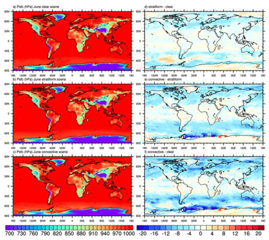
Figure 1.
The surface pressure SD background fields in June. (a–c) Surface pressure under clear, stratiform, and convective weather conditions, respectively. (d–f) The difference between stratiform and clear, convective and stratiform, and convective and clear, respectively.
The background covariance matrix represents the constraint relationship between various atmospheric parameters and varies from different weather conditions. The convection processes exhibit larger correlations between atmospheric variables in the troposphere. As the purpose of this study is to test the retrieval accuracy under TC conditions, the SD background covariance matrices are generated over oceans for three different weather scenes (clear, stratiform, and convective) in the same way as the background field. In addition, five atmospheric variables are taken into account in generating our SD background covariance matrices of temperature (T), humidity (Q), cloud water (CW), rain water (RW), and graupel water (GW). Considering that this study focuses on the retrieval under tropical cyclones conditions, the covariances of T and Q are calculated based on the ERA5 reanalysis dataset at low latitudes (30°S–30°N), while the covariances of hydrometeor variables are calculated based on the WRF simulation results of typhoon LEKIMA between 6th and 8th August in 2019 during which the TC’s intensity varied from 25 m/s to 50 m/s (with a model horizontal resolution of 27 km and vertical model top at 1 hPa). The ERA5 profiles are classified into three categories (clear, stratiform, or convective) according to the CLWP (cloud liquid water path) and CIWP (cloud ice water path) in order to obtain the subset of profiles under different scenes, which is consistent with that used by [16]. As precipitation-related parameters could be obtained in the WRF outputs, the profiles with rain rates less than 0.1 mm/h are defined as the clear profiles, while the profiles with the maximum reflectivity greater than 35 dBZ are defined as the convective profiles, while the rest are stratiform profiles.
Figure 2 shows the SD background covariance matrices for clear (a), stratiform (b), and convective (c). Note that the covariances are transformed to correlation coefficients to achieve a straightforward interpretation. It is clear that with the enhancement of convection, the correlation coefficients of parameters in the troposphere increase, especially for T and Q. The background covariance matrix without considering weather scenes is also illustrated in Figure 2d, which is used as a control experiment to prove the impact of the SD background covariance matrix on retrieval accuracy.
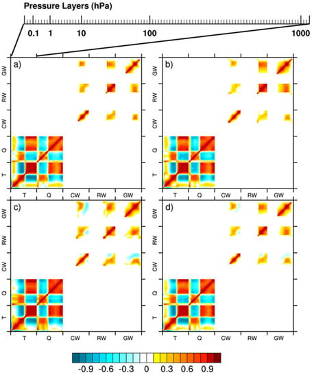
Figure 2.
The SD correlation coefficient for different weather conditions based on background covariances. (a–c) represent the relationship under clear, stratiform, and convective conditions, respectively, and (d) displays the correlation coefficient based on background covariances without considering weather conditions. Both the x- and y-axis represent the arrangement of different variables, as labeled beside the coordinate, from the top to the bottom layers, whose specific layers are shown at the top of this figure.
3.2. Scene Detection
The scene detection method is the basis for the SD 1DVAR algorithm. In this study, we only focus on cloud scene detection as the purpose is to retrieve the TCs’ structure over oceans. As the MWTS does not have 23.8 and 31.4 GHz channels that are sensitive to the cloud water path [26], new cloud detection methods were considered for FY-3D MW sounding instruments. Researchers have tried to detect the cloud scenes based on the bias-corrected observations-minus-backgrounds (O-B) of 50.3 GHz brightness temperature (BT) [13]. However, this method relied on atmospheric reanalysis data for the radiative transfer simulation to calculate the background BT [27], and the significance of performing the retrieval of atmospheric parameters on the premise that the reanalysis data are already available will be reduced. A comprehensive microwave sounder (CMWS) product was used in [16], which combined the MWTS and MWHS and simulated the missing 23.8 and 31.4 GHz channels based on the random forest model [28], and the cloud detection was performed similar to ATMS methods. However, the quality of this cloud detection method will depend on the accuracy of the simulated BT for the missing channels.
As this study was to retrieve the fusion data of the FY-3D MWTS and MWHS, the cloud emission and scattering index (CESI) based on the paired dual oxygen absorption bands located near 60 GHz and 118 GHz can be used for cloud detection [29]. The CESI can be briefly introduced as follows:
where and are the observed BT of paired MWTS and MWHS channels, respectively; is the regressed brightness temperatures of corresponding MWHS channels under clear conditions; and are the regression coefficients. In this study, we inherit the three groups of paired dual oxygen absorption bands from [29] representing the CESI at low (MWTS CH03 + MWHS CH07), middle (MWTS CH05 + MWHS CH06), and high (MWTS CH06 + MWHS CH05) layers. The regression coefficients and are generated based on four months’ (January, April, July, and October in 2018) clear condition fitting. The CESI is used to identify the weather conditions of FOVs into three categories: clear, stratiform, and convective scenes, to match the background fields and covariance matrices in SD 1DVAR. The thresholds for the classification are as follows:
where , , and represent the CESI calculated based on paired dual oxygen absorption bands for low, middle, and high layers [29], respectively. Figure 3 shows an example of cloud detection results at near 6:00 UTC on 14 September 2018, when Typhoon Mangkhut was active on the ocean east of the Philippines. Figure 3a,b display the scene detection results from ATMS based on the algorithm described in [16] and MWTS+MWHS based on CESI, respectively. Figure 3c shows the true color image from the VIIRS (Visible Infrared Imaging Radiometer Suite) onboard the Suomi NPP satellite at the same time. Although the cloud scenes identified by CESI have some clutters in low-latitude regions (may be caused by the incomplete uniformity of the spatial pixel observation positions when MWTS and MWHS are collocated), its clear and cloudy areas are basically the same as those in Figure 3a. In addition, the inner core structure and spiral rain band of Typhoon Mangkhut can be clearly depicted in Figure 3a,b, and the cloud system distribution is basically consistent with the VIIRS observations. These results indicate that with CESI method, FY-3D MW sounding instruments could achieve the cloud scene detection with a similar quality to those from the ATMS, even though the MWTS does not have 23.8 and 31.4 GHz channels.
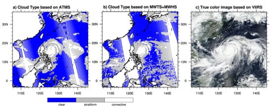
Figure 3.
The cloud scene detection results at near 6:00 UTC on 14 September 2018 from ATMS (a) and FY-3D MWTS+MWHS (b), with blue, grey, and white dots representing clear, stratiform, and convective scenes, respectively. (c) True color image at the same time from VIIRS onboard NPP satellite.
3.3. Bias Correction
Similar to [16], the bias correction method used in this study is also based on [30]. The specific scheme is as follows:
where is the biases of BT at each channel, defined as the radiative transfer model simulated BT minus observed BT; is the zenith angle; coefficients are fitted using the least squares method based on and . The ERA5 reanalysis dataset on the 2nd of every month from June 2018 to May 2019 is utilized as the input of the radiative transfer model to calculate the simulated BT. To investigate the influence of the observation operator, both CRTM and ARMS are used as radiative transfer models, and the bias correction coefficients are fitted for each model. Figure 4 takes MWTS Channel 5 at 54.4 GHz (a) and MWHS Channel 1 at 89 GHz (b) as examples to show the performances of our bias correction method. The systematic bias from the radiative transfer model, and the angle-dependent bias related to the instrument itself [30], can be corrected at the same time. The corrected bias is basically distributed around 0 and changes little with the local zenith angle. Meanwhile, the observation operator error, defined as the standard deviation of O-B, is not affected by the bias correction, as shown in the red and blue shaded areas in Figure 4.
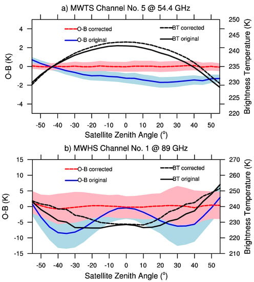
Figure 4.
The bias correction results of MWTS channel 5 (a) and MWHS channel 1 (b). Solid and dashed black curves represent the averaged original and corrected BT as a function of satellite zenith angle, respectively. Red and blue curves represent the averaged original and corrected O-B as a function of satellite zenith angle, respectively. Red and blue shaded areas represent the range of one standard deviation centered on the corrected and original O-B mean value as a function of satellite zenith angle, respectively.
4. Results
4.1. Effects of SD Background Covariance Matrices on 1DVAR Retrieval
Two experiments are set to test the effects of SD background covariance matrices on the retrieved TC’s thermal structures, as shown in Table 2. In EXP_noSDCov, the background covariance matrix without considering the cloud scenes (Figure 2d) is used in 1DVAR retrieval, while the SD background covariance matrices (Figure 2a–c) are used in EXP_SDCov retrievals. Note that both of these experiments use the SD background fields as introduced in [16] and Section 3.1, and all channels from MWTS and MWHS are used in the 1DVAR retrievals. ARMS is used as the observation operator in this study.

Table 2.
Description of experiments for different background covariance matrices.
As stated in Section 2.2, we retrieve 489 records of 41 TCs from 2018 to 2020. In order to visually display the retrieved TC vertical thermal structures, we select four records of different intensity levels as examples, whose minimum center surface pressures are 992, 978, 951, and 938 hPa, specifically. Figure 5 and Figure 6 show the results from EXP_SDCov and EXP_noSDCov, respectively, with subplots a-d and e-h representing the retrieved TC anomalies of temperature and humidity, respectively. Following [9], the temperature anomaly is calculated by the difference between the local air temperature and the azimuthal mean temperature (averaged in the 550–650 km annulus from the storm center) at each corresponding layer. The scattering-related unexpected cold anomaly errors in the lower layers, as appearing in some previous studies [10,11], are eliminated in both EXP_SDCov and EXP_noSDCov, and the warm core center warms up with the TC intensity, which is consistent with theoretical studies [9] and previous observation results [11,12]. The retrieved humidity distributions are also reasonable in both EXP_SDCov and EXP_noSDCov, with the large humidity appearing at lower layers and decreasing with height. The humidity is also higher in the inner region of TCs, which is also consistent with the theoretical results as the strong convection is more likely to appear in the inner region, leading to a larger water content in this area.
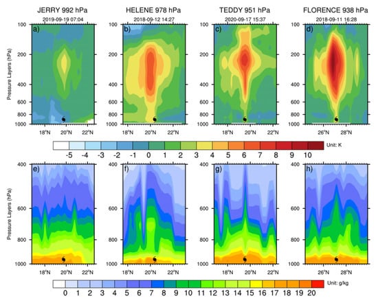
Figure 5.
Retrieved vertical distribution of temperature anomaly (a–d) and humidity (e–h) of four TC records from EXP_SDCov. The TC name, intensity, as well as its observation time are listed on the top of every column. The hurricane symbols indicate the center of hurricanes.
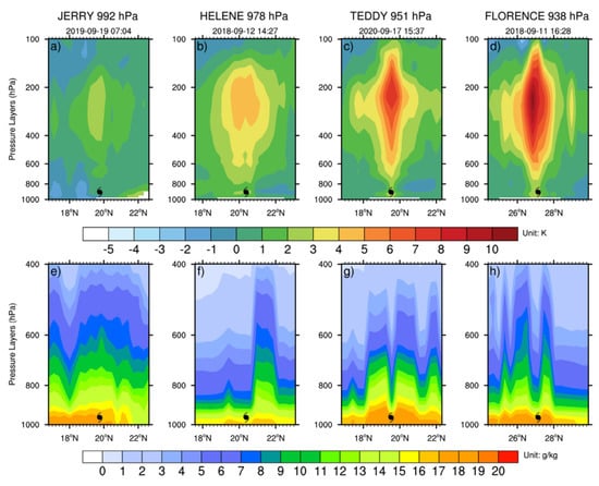
Figure 6.
Same as Figure 5, except for temperature anomaly (a–d) and humidity (e–h) structures retrieved from EXP_noSDCov.
All the retrieval experiments reveal reasonable temperature and humidity structures for any stages of TC and are consistent with [16]. Using only the SD background field could result in a good thermal structure of TCs. However, spotted differences are shown between EXP_SDCov and EXP_noSDCov, especially for the humidity fields, which might be the result of the SD background covariance matrices. At this stage, it is difficult to judge the results in Figure 5 and Figure 6. Thus, the validation against direct observations of a large sample size is given in the following section to obtain the quantitative statistical conclusions.
Temperature and humidity profiles retrieved from both EXP_SDCov and EXP_noSDCov are compared with flight dropsonde observations. As the specific humidity changes significantly with height, we use the relative humidity for better illustration. Figure 7 displays the vertical distribution of mean bias (defined as flight observed profiles minus 1DVAR retrieved profiles, blue curves) and RMSE (root-mean-squared error, red curves) from both EXP_SDCov (solid curves) and EXP_noSDCov (dashed curves). Figure 7a,b represent the results for temperature and humidity, respectively. Note that dropsonde data in the inner-region of TCs are only available below 700 hPa, resulting in the decrease in sample size between 850 and 700 hPa, and the sudden change in temperature error around 700 hPa (Figure 7a) could also be attributed to the decrease in inner-region samples where large scattering conditions are more likely to occur.
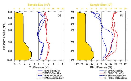
Figure 7.
Validation results for retrieved temperature (a) and relative humidity (b) products based on flight dropsonde observations. Blue and red curves represent the mean bias and RMSE results, respectively. Solid and dashed curves represent validation from EXP_SDCov and EXP_noSDCov, respectively. The yellow shaded areas corresponding to the top axis represent the number of the collocated retrieval profiles with the dropsonde observations, which change with vertical layers as the airplane flight levels vary from observation locations.
Overall, the temperature bias and RMSE are concentrated around 0.5 K and 1.5 K, respectively, for both EXP_SDCov and EXP_noSDCov, except for higher layers around 300 hPa (layers of warm core area), where the bias of EXP_noSDCov could reach as large as 1.3 K, which means that the retrieved warm core intensity might be weaker than the true value. As a comparison with NOAA MiRS retrieval errors of 2–4 K under TC conditions [5], the temperature accuracy in this study is greatly improved. Meanwhile, using SD background covariance matrices could reduce the bias and RMSE by around 0.5 K near 300 hPa. Though the low-layer bias and RMSE are similar between these two experiments, the errors are also slightly reduced by about 0.2 K after using SD background covariances. The improvement of humidity accuracy is more significant compared with temperature, which is consistent with those shown in Figure 5 and Figure 6. As shown in Figure 7b, the RMSE of humidity is reduced by 10–15% in the layer from 850 to 500 hPa after using SD background covariances, and the larger bias between these layers is also reduced by 10–20%. As water vapor content is more concentrated in this region, this improvement is very important for the accurate monitoring of TC’s water vapor structure.
4.2. Effects of Observation Operator on 1DVAR Retrieval
Considering that ARMS is a newly developed radiative transfer model, it’s the first time ARMS has been used as an observation operator in variational retrievals. As CRTM is a commonly used observation operator in retrieval systems such as in [16,17,18], this study compares the uses of ARMS and CRTM and understands the influence of different radiative transfer models on the retrieved accuracy under TC conditions. Meanwhile, analysis of SD background covariance matrices is also conducted for both operators. Therefore, we design four sets of experiments, as shown in Table 3. Note that experiments EXP_ noSDCov_ARMS and EXP_SDCov_ARMS are similar to EXP_noSDCov and EXP_SDCov, respectively, as described in Section 4.1, and all the experiments use scene-dependent background fields, as described in [16].

Table 3.
Experiments for different background covariance matrices and observation operators.
Figure 8 shows assessments of temperature (a) and humidity (b) profiles retrieved using static (dashed curves) or SD (solid curves) background covariance matrices. As with as Figure 7, the upper troposphere temperature errors, as well as the mid- to low- troposphere relative humidity errors, are reduced after using SD background covariances. The temperature reduction could reach up to 1 K and 0.5 K for bias and RMSE, respectively. The humidity error reduction is significantly large, with bias and RMSE reduced by 15% and 10%, respectively, at mid- to low-troposphere, which is consistent with previous results using ARMS as the operator. This means that the SD background covariance matrices algorithm could improve the retrieval accuracy using either CRTM or ARMS as the observation operator.
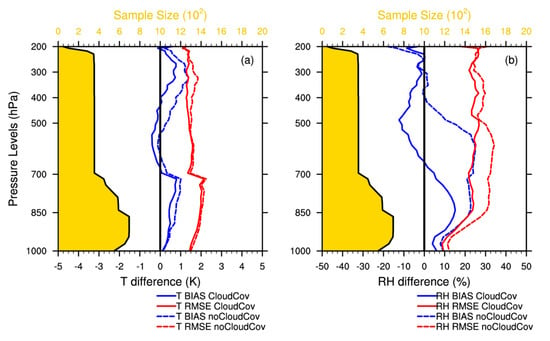
Figure 8.
Same as Figure 7, except for validation results for retrieved temperature (a) and relative humidity (b) products using CRTM as the observation operator.
Differences still exist from using these two radiative transfer models. In Figure 9, the temperature bias and RMSE are almost the same after replacing CRTM with ARMS as an observation operator. Considering the small temperature retrieval errors under TC conditions from these two experiments (bias and RMSE are around 0.5 and 1.5–2 K, respectively), the room for improvement is limited due to the influence of the noise and resolution of the instruments themselves. Meanwhile, the relative humidity errors show differences between these two experiments. After using ARMS as an observation operator, the relative humidity error can be further reduced by up to 5% (at layers around 850 hPa) compared with CRTM results, and the bias is closer to 0 in ARMS results, especially for mid- to high-layers (Figure 9b). Considering that these two experiments share similar humidity errors when using the static background covariances matrix (Figure 8b), this indicates that using ARMS as an observation operator could take full advantage of the SD background covariance matrices to reduce the humidity retrieval error under strong scattering conditions. As the nonspherical particles are considered using discrete dipole approximation when training MW scattering coefficients in ARMS, the MW-related scattering process is considered more comprehensive in the forward and adjoint calculation in ARMS compared with CRTM [22]. Considering that water vapor absorption channels of MWHS are located at frequencies near 183 GHz, which are more affected by particle scattering, compared with oxygen absorption channels at frequencies near 50–60 GHz or 118.75 GHz), the advanced consideration of scattering effects in ARMS could lead to more accurate forward and adjoint simulations of water vapor absorption channels, and then to the smaller errors in humidity retrievals, as shown in Figure 9b.
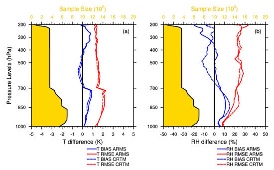
Figure 9.
Validation results for retrieved temperature (a) and relative humidity (b) products from different observation operators based on flight dropsonde observations using SD background covariance matrices. Blue and red curves represent mean bias and RMSE results, respectively. Solid and dashed curves represent validation from EXP_SDCov_ARMS and EXP_SDCov_CRTM, respectively. The yellow shaded areas corresponding to the top axis represent the number of the collocated retrieval profiles with the dropsonde observations, which change with vertical layers as the airplane flight levels vary from observation locations.
In order to compare the differences between ARMS and CRTM under cloudy conditions, we select the MWHS data on the 2nd day of every month from June to October in 2018 to conduct the forward simulation experiments. The atmospheric parameters for the radiative transfer model are obtained from the ERA5 reanalysis data, and the cloud parameters are from the Level 2A GPROF (Goddard Profiling Algorithm) cloud microphysics profile product of Global Precipitation Measurement (GPM) Microwave Imager (GMI) [31], which are temporally and spatially collocated with the MWHS FOVs. Note that only FOVs over oceans are simulated, and only the GMI products with their pixel centered within MWHS FOVs and the difference between the observation time less than 15 min are collocated. Considering the GMI microphysical products contain four hydrometers (cloud water, cloud ice, rain, and snow), in this study, we only consider liquid and solid hydrometers, that is, cloud water and cloud ice when there is no precipitation, and rain and snow when precipitation occurs.
Figure 10 and Figure 11 show the comparison between observed and simulated BT under no precipitation and precipitation conditions, respectively. Four MWHS channels are chosen as examples, including two window channels (89 GHz and 150 GHz) and two water vapor absorption channels (around 183.31 GHz). In addition, the mean bias and the standard deviation of the observation minus simulations BT (O-B) are also shown in those figures. As shown in Figure 10, the mean bias and standard deviations of O-B from ARMS and CRTM are close under nonprecipitation cloudy conditions. The simulation accuracy of the two models decreases due to the effect of heavy precipitation particle scattering under precipitation conditions (as shown in Figure 11), but some differences can be spotted between these two models. ARMS-simulated O-B tend to have a smaller bias and standard deviation for most channels compared with CRTM results, except for the 89 GHz channel, and the improvement is more pronounced in the water vapor absorption channels. This further explains the improved accuracy of water vapor retrievals after using ARMS as the observation operator, as shown in Figure 9.
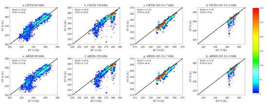
Figure 10.
Scatter density plots of observed and simulated BT for 4 MWHS channels under no precipitation cloud conditions from CRTM (a–d) and ARMS (e–h). Shaded colors represent the sample size within every 1 × 1 K bin.
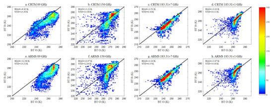
Figure 11.
Similar to Figure 10, except for results under precipitation conditions. Both results from CRTM (a–d) and ARMS (e–h) are shown.
5. Discussion and Conclusions
This study proposes a scene-dependent (SD) variational retrieval method with the background profiles and their covariance matrices varying with atmospheric scattering conditions. The algorithm effectiveness is demonstrated through uses of the FY-3D microwave (MW) sounding instruments under tropical cyclone (TC) conditions. Assessments based on flight dropsonde observations show that the temperature and humidity errors are around 1.5 K and 10–20%, respectively, throughout the troposphere. After using the SD background covariance matrices, both the temperature and relative humidity errors are reduced up to 0.5 K and 15%, respectively. The most improved temperature layers are near 300 hPa, where the TC warm core center is often located, while the humidity errors significantly decrease at mid- to low-troposphere layers where the water vapor content is mostly concentrated. These results indicate that SD background covariances can resolve warm core and humidity more accurately, compared to the previous studies.
The influences from observation operators on variational retrieval errors are also analyzed in this study. The assessment results show that the SD variational method could improve the retrieval accuracy using either CRTM or ARMS as an observation operator. Benefiting from the more comprehensive calculation of MW-related scattering processes in ARMS, the accuracy of the retrieved humidity under TC conditions is improved after replacing the observation operator from CRTM to ARMS. The bias of humidity error is closer to 0, and the RMSE is reduced by up to 5% after using ARMS in variational retrievals. These results indicate that the comprehensive consideration of the scattering effect of nonspherical particles in the radiative transfer model could improve the application of MW data under cloudy and precipitation conditions, especially for high-frequency MW data, in variational calculations. This is important for the development of the radiative transfer model, as well as for variational retrieval and data assimilation of MW sounding instruments.
In addition to temperature and humidity, the SD variational inversion algorithm also relies on the background field and background covariance matrix of different hydrometeors. The hydrometeor profiles including cloud water (CW), rain water (RW), and graupel water (GW) are generated from WRF model outputs. However, as WRF hydrometeor profiles are dependent on microphysical schemes, the impact of the hydrometeor background fields and background covariance matrices used in our 1DVAR algorithm on the final products is subject to more investigation. In fact, in order to improve the simulation accuracy of the radiative transfer model under cloudy conditions, the hydrometeor parameters are mainly used to characterize the atmospheric scattering conditions in our algorithm. As this article focuses on the retrieval of TCs’ temperature and humidity structure, the hydrometeors products are not discussed. Depending on the retrieved high-quality temperature and humidity profiles from this work, our next step will focus on the retrieval of hydrometeor profiles under cloudy and rainy conditions, as well as the influence from different cloud microphysical schemes on the hydrometeor covariance matrices and the retrieval results.
Author Contributions
Conceptualization, H.H. and F.W.; methodology, H.H. and F.W.; validation, H.H.; writing—original draft preparation, H.H.; writing—review and editing, F.W. All authors have read and agreed to the published version of the manuscript.
Funding
This research was funded by the National Key Research and Development Program of China (2021YFB3900400), the National Natural Science Foundation of China (42105136, U2142212), and the Basic Research Fund of CAMS (2020Y013).
Institutional Review Board Statement
Not applicable.
Informed Consent Statement
Not applicable.
Data Availability Statement
The FY3D satellite data can be downloaded from the website of China National Satellite Meteorological Center (http://satellite.nsmc.org.cn/portalsite/default.aspx, accessed on 27 December 2021). The hurricane best-track dataset can be downloaded from the website of the National Hurricane Center (www.nhc.noaa.gov/data/#hurdat, accessed on 27 December 2021). The flight dropsonde dataset can be downloaded from the website of the Hurricane Research Division (www.aoml.noaa.gov/hrd/data_sub/dropsonde.html, accessed on 27 December 2021). The level 2A GMI GPROF dataset can be downloaded from the website of NASA STORM (https://storm.pps.eosdis.nasa.gov/storm/, accessed on 27 December 2021).
Acknowledgments
We thank Jun Yang, Yang Han, and Yining Shi for supporting the usage of the ARMS radiative transfer model. We would also like to thank the reviewers and the editors for their valuable and helpful suggestions.
Conflicts of Interest
The authors declare no conflict of interest.
References
- Dvorak, V.F. Tropical Cyclone Intensity Analysis Using Satellite Data; US Department of Commerce, National Oceanic and Atmospheric Administration: Silver Spring, MD, USA, 1984; Volume 11. [Google Scholar]
- Velden, C.; Harper, B.; Wells, F.; Beven, J.L.; Zehr, R.; Olander, T.; Mayfield, M.; Guard, C.C.; Lander, M.; Edson, R.; et al. The dvorak tropical cyclone intensity estimation technique: A satellite-based method that has endured for over 30 years. Bull. Am. Meteorol. Soc. 2006, 87, 1195–1210. [Google Scholar] [CrossRef]
- Vigh, J.L.; Schubert, W.H. Rapid development of the tropical cyclone warm core. J. Atmos. Sci. 2009, 66, 3335–3350. [Google Scholar] [CrossRef] [Green Version]
- Komaromi, W.A.; Doyle, J.D. Tropical cyclone outflow and warm core structure as revealed by HS3 dropsonde data. Mon. Weather. Rev. 2017, 145, 1339–1359. [Google Scholar] [CrossRef]
- Gao, S.; Wang, D.; Hong, H.; Wu, N.; Li, T. Evaluation of warm-core structure in reanalysis and satellite data sets using HS3 dropsonde observations: A case study of hurricane edouard (2014). J. Geophys. Res. Atmos. 2018, 123, 6713–6731. [Google Scholar] [CrossRef]
- Kidder, S.Q.; Goldberg, M.D.; Zehr, R.M.; DeMaria, M.; Purdom, J.F.W.; Velden, C.S.; Grody, N.C.; Kusselson, S.J. Satellite analysis of tropical cyclones using the advanced microwave sounding unit (AMSU). Bull. Am. Meteorol. Soc. 2000, 81, 1241–1260. [Google Scholar] [CrossRef] [Green Version]
- Weng, F.; Zou, X.; Sun, N.; Yang, H.; Tian, M.; Blackwell, W.J.; Wang, X.; Lin, L.; Anderson, K. Calibration of Suomi national polar-orbiting partnership advanced technology microwave sounder. J. Geophys. Res. Atmos. 2013, 118, 11187–111200. [Google Scholar] [CrossRef]
- Knaff, J.A.; Seseske, S.A.; DeMaria, M.; Demuth, J.L. On the influences of vertical wind shear on symmetric tropical cyclone structure derived from AMSU. Mon. Weather. Rev. 2004, 132, 2503–2510. [Google Scholar] [CrossRef] [Green Version]
- Stern, D.P.; Nolan, D.S. On the height of the warm core in tropical cyclones. J. Atmos. Sci. 2012, 69, 1657–1680. [Google Scholar] [CrossRef]
- Tian, X.; Zou, X. Capturing size and intensity changes of hurricanes irma and maria (2017) from polar-orbiting satellite microwave radiometers. J. Atmos. Sci. 2018, 75, 2509–2522. [Google Scholar] [CrossRef]
- Lin, L.; Weng, F. Estimation of hurricane maximum wind speed using temperature anomaly derived from advanced technology microwave sounder. IEEE Geosci. Remote Sens. Lett. 2018, 15, 639–643. [Google Scholar]
- Wang, X.; Jiang, H. A 13-year global climatology of tropical cyclone warm-core structures from AIRS data. Mon. Weather. Rev. 2019, 147, 773–790. [Google Scholar] [CrossRef]
- Niu, Z.; Zou, X.; Huang, W. Typhoon warm-core structures derived from FY-3D MWTS-2 observations. Remote Sens. 2021, 13, 3730. [Google Scholar] [CrossRef]
- Quanhua, L.; Fuzhong, W. One-dimensional variational retrieval algorithm of temperature, water vapor, and cloud water profiles from advanced microwave sounding unit (AMSU). IEEE Trans. Geosci. Remote Sens. 2005, 43, 1087–1095. [Google Scholar] [CrossRef]
- Han, Y.; Weng, F. Remote sensing of tropical cyclone thermal structure from satellite microwave sounding instruments: Impacts of optimal channel selection on retrievals. J. Meteorol. Res. 2018, 32, 804–818. [Google Scholar] [CrossRef]
- Hu, H.; Han, Y. Comparing the thermal structures of tropical cyclones derived from suomi NPP ATMS and FY-3D microwave sounders. IEEE Trans. Geosci. Remote Sens. 2021, 59, 8073–8083. [Google Scholar] [CrossRef]
- Hu, H.; Weng, F.; Han, Y.; Duan, Y. Remote sensing of tropical cyclone thermal structure from satellite microwave sounding instruments: Impacts of background profiles on retrievals. J. Meteorol. Res. 2019, 33, 89–103. [Google Scholar] [CrossRef]
- Boukabara, S.-A.; Garrett, K.; Chen, W.; Iturbide-Sanchez, F.; Grassotti, C.; Kongoli, C.; Chen, R.; Liu, Q.; Yan, B.; Weng, F. MiRS: An all-weather 1DVAR satellite data assimilation and retrieval system. IEEE Trans. Geosci. Remote Sens. 2011, 49, 3249–3272. [Google Scholar] [CrossRef]
- Grassotti, C.; Liu, S.; Lee, Y.-K.; Liu, Q. Preliminary development and assessment of the NOAA microwave integrated retrieval system for tropical cyclones (MiRS-TC): A passive satellite microwave retrieval algorithm optimized for the tropical cyclone environment. In Proceedings of the AGU Fall Meeting, College Park, MD, USA, 24–28 February 2020. [Google Scholar]
- Weng, F.; Yu, X.; Duan, Y.; Yang, J.; Wang, J. Advanced radiative transfer modeling system (ARMS): A new-generation satellite observation operator developed for numerical weather prediction and remote sensing applications. Adv. Atmos. Sci. 2020, 37, 131–136. [Google Scholar] [CrossRef] [Green Version]
- Shi, Y.-N.; Yang, J.; Weng, F. Discrete Ordinate Adding Method (DOAM), a new solver for Advanced Radiative transfer Modeling System (ARMS). Opt. Express 2021, 29, 4700–4720. [Google Scholar] [CrossRef]
- Yang, J.; Weng, F. Analysis of Microwave scattering properties of non-spherical ice particles using discrete dipole approximation. In Proceedings of the IGARSS 2020—2020 IEEE International Geoscience and Remote Sensing Symposium, Waikoloa, HI, USA, 26 September–2 October 2020; pp. 5309–5312. [Google Scholar]
- Hou, X.; Han, Y.; Hu, X.; Weng, F. Verification of fengyun-3D MWTS and MWHS calibration accuracy using GPS radio occultation data. J. Meteorol. Res. 2019, 33, 695–704. [Google Scholar] [CrossRef]
- Zhang, S.; Li, J.; Wang, Z.; Wang, H.; Sun, M.; Jiang, J.; He, J. Design of the second generation microwave humidity sounder (MWHS-II) for Chinese meteorological satellite FY-3. In Proceedings of the 2012 IEEE International Geoscience and Remote Sensing Symposium, Munich, Germany, 22–27 July 2012; pp. 4672–4675. [Google Scholar]
- Landsea, C.W.; Franklin, J.L. Atlantic hurricane database uncertainty and presentation of a new database format. Mon. Weather. Rev. 2013, 141, 3576–3592. [Google Scholar] [CrossRef]
- Grody, N.; Zhao, J.; Ferraro, R.; Weng, F.; Boers, R. Determination of precipitable water and cloud liquid water over oceans from the NOAA 15 advanced microwave sounding unit. J. Geophys. Res. Atmos. 2001, 106, 2943–2953. [Google Scholar] [CrossRef]
- Niu, Z.; Zou, X.; Ray, P.S. Development and testing of a clear-sky data selection algorithm for FY-3C/D microwave temperature sounder-2. Remote Sens. 2020, 12, 1478. [Google Scholar] [CrossRef]
- Han, Y.; Yang, J.; Hu, H.; Dong, P. Retrieval of oceanic total precipitable water vapor and cloud liquid water from fengyun-3d microwave sounding instruments. J. Meteorol. Res. 2021, 35, 371–383. [Google Scholar] [CrossRef]
- Han, Y.; Zou, X.; Weng, F. Cloud and precipitation features of Super Typhoon Neoguri revealed from dual oxygen absorption band sounding instruments on board FengYun-3C satellite. Geophys. Res. Lett. 2015, 42, 916–924. [Google Scholar] [CrossRef]
- Weng, F.; Zhao, L.; Ferraro, R.R.; Poe, G.; Li, X.; Grody, N.C. Advanced microwave sounding unit cloud and precipitation algorithms. Radio Sci. 2003, 38, 33-1–33-13. [Google Scholar] [CrossRef]
- Kummerow, C.D.; Randel, D.L.; Kulie, M.; Wang, N.-Y.; Ferraro, R.; Joseph Munchak, S.; Petkovic, V. The evolution of the goddard profiling algorithm to a fully parametric scheme. J. Atmos. Ocean. Technol. 2015, 32, 2265–2280. [Google Scholar] [CrossRef]
Publisher’s Note: MDPI stays neutral with regard to jurisdictional claims in published maps and institutional affiliations. |
© 2022 by the authors. Licensee MDPI, Basel, Switzerland. This article is an open access article distributed under the terms and conditions of the Creative Commons Attribution (CC BY) license (https://creativecommons.org/licenses/by/4.0/).