Article

Combining Spectral and Textural Information from UAV RGB Images for Leaf Area Index Monitoring in Kiwifruit Orchard

College of Natural Resources and Environment, Northwest A&F University, Yangling 712100, China
*
Author to whom correspondence should be addressed.
Remote Sens. 2022, 14(5), 1063; https://doi.org/10.3390/rs14051063
Submission received: 12 January 2022 / Revised: 17 February 2022 / Accepted: 18 February 2022 / Published: 22 February 2022
(This article belongs to the Special Issue Advances of Remote Sensing in Precision Agriculture)

Abstract

:
The use of a fast and accurate unmanned aerial vehicle (UAV) digital camera platform to estimate leaf area index (LAI) of kiwifruit orchard is of great significance for growth, yield estimation, and field management. LAI, as an ideal parameter for estimating vegetation growth, plays a significant role in reflecting crop physiological process and ecosystem function. At present, LAI estimation mainly focuses on winter wheat, corn, soybean, and other food crops; in addition, LAI on forest research is also predominant, but there are few studies on the application of orchards such as kiwifruit. Concerning this study, high-resolution UAV images of three growth stages of kiwifruit orchard were acquired from May to July 2021. The extracted significantly correlated spectral and textural parameters were used to construct univariate and multivariate regression models with LAI measured for corresponding growth stages. The optimal model was selected for LAI estimation and mapping by comparing the stepwise regression (SWR) and random forest regression (RFR). Results showed the model combining texture features was superior to that only based on spectral indices for the prediction accuracy of the modeling set, with the R2 of 0.947 and 0.765, RMSE of 0.048 and 0.102, and nRMSE of 7.99% and 16.81%, respectively. Moreover, the RFR model (R2 = 0.972, RMSE = 0.035, nRMSE = 5.80%) exhibited the best accuracy in estimating LAI, followed by the SWR model (R2 = 0.765, RMSE = 0.102, nRMSE = 16.81%) and univariate linear regression model (R2 = 0.736, RMSE = 0.108, nRMSE = 17.84%). It was concluded that the estimation method based on UAV spectral parameters combined with texture features can provide an effective method for kiwifruit growth process monitoring. It is expected to provide scientific guidance and practical methods for the kiwifruit management in the field for low-cost UAV remote sensing technology to realize large area and high-quality monitoring of kiwifruit growth, thus providing a theoretical basis for kiwifruit growth investigation.

Graphical Abstract

1. Introduction

UAV remote sensing (RS) plays an outstanding role in precision agriculture due to its convenient, fast, and accurate acquisition of surface information [1]. Hyperspectral and multispectral remote sensing platforms carried by UAVs are widely used in professional fields or departments such as land and scientific research; however, on account of the complexity and redundancy in the post-processing stage of hyperspectral data, its application in the common farming environment is limited to some extent [2,3]. Some additional methods of crop growth monitoring have gradually emerged lately owing to the enhanced affordability and accessibility of the drones with multispectral imaging, especially digital cameras [4]. To date, several studies have indicated that drones equipped with digital cameras played an irreplaceable role in crop growth monitoring, which was commonly represented using parameters of growth condition such as leaf area index [5], leaf chlorophyll content [6], biomass [7], yield [8,9], leaf nitrogen content [10], nitrogen nutrition index [11], water content [12], etc. Furthermore, there were also some examples of UAV-based analysis on the vegetated water ways [13,14,15], and some applications of machine learning approaches in agricultural and geoscience research [16,17,18]. In particular, real-time dynamic monitoring of LAI is of great significance to crop growth diagnosis and management regulation.
Leaf area index (LAI) is defined as the total area of photosynthesis in a one-sided plant per unit of land area, which can be understood as the ratio of the total leaf area of plants to the land area [19]. LAI, as an ideal parameter for estimating vegetation growth, plays an individual role in reflecting crop physiological process and ecosystem function [20]. In general, the direct measurement of LAI causes great damage to crops and is time-consuming and labor-intensive; at the same time, sampling is subjective and unrepresentative, which makes it difficult to achieve large-scale overall monitoring. Indirect measurement methods such as optical instruments based on Beer-Lambert Law can precisely measure LAI by measuring the extinction coefficient of vegetation accurately in the region [21]. Currently widely used optical instruments can be divided into two methods according to principle, which are based on radiation and image measurement respectively. Representative instruments of the former are LAI-2000 (Licor Inc., Lincoln, NE, USA), Sunscan (Delta-T Inc., Cambridge, UK), etc. The advantage of radiometric instruments is that they are fast and convenient to measure. However, they are susceptible to weather and often need to work in sunny weather [22]. Typical instruments based on image measurement are CI-110 (CID Inc., Washington, DC, USA), WinScanopy (Regent Inc., Thunder Bay, Canada), etc. With the innovation of technology, the image measurement method represented by CI-110 has higher measurement accuracy than the radiation measurement method represented by LAI-2000; meanwhile, the need for a specific measurement environment is greatly reduced, which is especially suitable in the monitoring of forest and fruit trees [23]. Because kiwifruit is different from ordinary crops in its planting structure and pattern, such as its thin stem, large leaves, and unique growth period, the non-destructive measurement of LAI in kiwifruit orchards is relatively more difficult [24]. CI-110 is suitable for LAI exploration of low lying plant canopies up to forest canopy through the measurement of sunflecks in the range of photosynthetically active radiation (PAR), and the calculation of diffuse radiation transmission coefficients (the sky view factor), mean foliage inclination angles, and plant canopy extinction coefficients [25,26]. At present, there are few reports on the kiwifruit orchards by CI-110; therefore, the application of CI-110 in nondestructive, accurate, and rapid LAI monitoring is of great significance for breeding and guiding the production of kiwifruit with high quality. Drones can also overcome these ground measurement problems and have practical significance in the precise management of kiwifruit orchards.
In the research of precision agriculture, RS platform mainly focuses on the estimation of chlorophyll content [6,27], nitrogen content [11,28], LAI [29,30], and biomass [9,31] of winter wheat [32,33], corn [34,35], soybean [36], and other food crops. However, LAI studies on orchards such as kiwifruit are rarely involved. In terms of research methods, it is common to use spectral index, texture, plant height, and other parameters to construct an estimation model [28,37,38]. As an important characteristic, texture is not only used to identify objects or regions of interest in images and image classification [39,40,41], but also used to estimate forest [42,43] and some crops [33,37]. However, texture in the UAV imagery was rarely used for orchards monitoring. The primary objective of this investigation was to predict LAI in the kiwifruit orchard using the color and texture feature extracted from UAV high-resolution RGB images of the study area. A secondary objective was to verify whether the model with spectral indices combining texture features was more beneficial to LAI estimation.

2. Materials and Methods

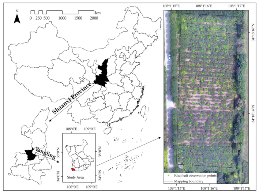
2.1. Study Area Overview

The study was performed in a kiwi orchard located in Yangling Agricultural High-tech Demonstration Zone, Shaanxi Province, China (108°01′32′′ E, 34°18′09′′ N) (Figure 1). This area has a temperate, continental, and semiarid climate. The average annual precipitation and average annual temperature are 649.5 mm and 12.9 °C, respectively. In this experiment, 80 kiwifruits with similar tree age and suitable growing conditions in the kiwi orchard were selected as the study samples, which were sampled in the initial flowering stage (IF), young fruit stage (YF), and fruit enlargement stage (FE) in 2021.

2.2. Data Acquisition

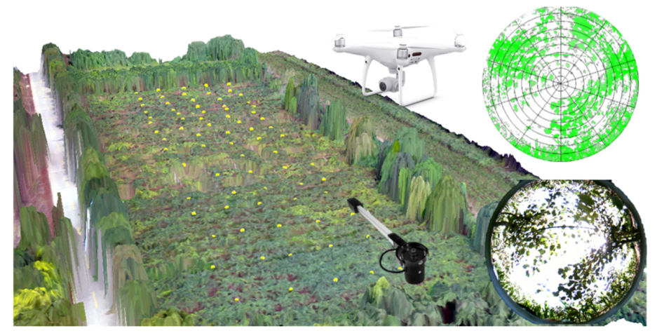
2.2.1. LAI Measurement of Kiwi Orchard

The Plant Canopy Imager CI-110 (CID Inc., Washington, DC, USA) was used to make two observations on the same horizontal plane (about 0.5 m above the ground) below the canopy of each sampling point, and the average value was taken as the LAI value of the sampling [44]. The length is 0.84 m, and the imaging probe and arm weigh 1.5 kg. It is equipped with a 170° fisheye lens with an image resolution of 8 million pixels. LAI was calculated using the CI-110 Plant Canopy Analysis software (https://cid-inc.com/, accessed on12 January 2022). During image capture, the brightness (luminosity) and contrast (between background and foreground) were tuned to provide visual quality. The measured data were imported into the software for further processing and the ground observation values were derived. Figure S1 shows the observation of some growth periods. In addition, a global navigation satellite system (GNSS) receiver was used to locate each measuring sample point, and coordinated the point position with the actual position of the image.

2.2.2. UAV RGB Image Acquisition and Preprocessing

DJI Phantom 4 PRO quadcopter (SZ DJI Technology Co., Shenzhen, China) was used for aerial data acquisition. The take-off weight is 1.38 kg and the endurance time is approximately 30 min. The 1-inch CMOS sensor equipped with a 20-megapixel camera on the UAV platform obtained high-resolution visible-light images of the initial flowering stage, young fruit stage, and fruit enlargement stage respectively (Table 1). Each flight was completed between 10 a.m. and 2 p.m. when the sun was steady and clear with few clouds. DJI GS Pro platform, which supports route planning, was adopted to set the course and side overlap properties of this mission were set to 80%, at a height of 30 m from the ground. Agisoft PhotoScan Professional software (https://www.agisoft.com/, accessed on 12 January 2022) was applied to mosaic the obtained digital images. The software aligns the photos with the Position and Orientation System (POS), the coordinate system of which is WGS84, as recorded by the drone at the time of shooting, and generates a dense point cloud of the flight area. The spatial grid and texture are then established to obtain the digital elevation model (DEM) and digital orthophoto map (DOM) of the study area with a nominal resolution of 0.014 m mean ground sampling distance (GSD) at 30 m above ground level with reference to the WGS84/UTM zone 49N as a map projection method. Figure 2 displayed a 3-dimensional image in the study area by ArcGIS 10.6 and instrument CI-110 for LAI observation.

2.3. Methods

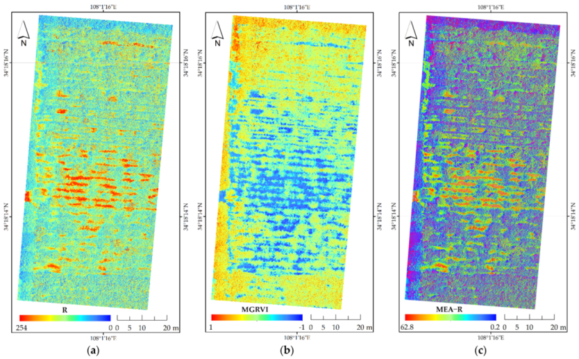
2.3.1. Extraction of Spectral and Texture Features

The average digital number (DN) values of the region of interest (ROI) from the orthorectified image were calculated by ArcGIS 10.6. The average DN value, normalized DN value, and other spectral indices related to LAI were selected based on the image characteristics of red (R), green (G), and blue (B) bands (Table 2). Gray Level Co-occurrence Matrix (GLCM) was used to calculate texture information by ENVI 5.2; that is, the frequency of pixels in the 3 × 3 window was calculated based on the second-order probability statistical filtering. There were 24 texture features in total in terms of eight statistical methods on each band (Table 3). In order to simplify the parameter name, underline and band name were added to distinguish the texture information of each band, for example, MEA_R represented the mean of the red band. A group of images in Figure 3 illustrate part of the parameters analyzed in the study, and more images of parameters are exhibited in Figure S2.

2.3.2. Model Calibration and Evaluation
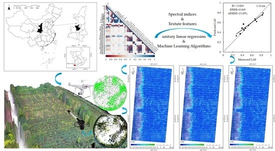
In the model training, we randomly selected 80% of the samples as the modeling data sets according to different growth periods. The parameters with the highest correlation with LAI were selected as the independent variable of estimation and LAI was selected as the dependent variable. Then LAI estimation was performed using univariate regression models including unary linear equation, unary quadratic polynomial equation, power function, and exponential and logarithmic function. Additionally, concerning multivariate regression models, machine learning algorithms (MLA) were adopted, such as stepwise regression and random forest regression. The remaining 20% of samples were used as validation sets to evaluate the prediction accuracy of the LAI estimation model.
In multivariate regression analysis, stepwise regression selects the optimal model by iteratively adding or deleting independent variables. At the same time, Akaike Information Criterion (AIC) is a weighting function of fitting accuracy and unknown number of parameters, which is used to measure the complexity and performance of the stepwise regression model. While pursuing the maximum likelihood of the model, the number of stepwise regression variables should be as small as possible. That is to say, the smaller the AIC, the better the model. In the training stage of random forest regression, bootstrap sampling is used to collect multiple different sub-training data sets from the input training data sets to train multiple different decision trees successively. In the prediction stage, the random forest averages the prediction results of all internal binary decision trees to obtain the final result. The benefit of bagging algorithms such as random forest is that they increase the robustness and stability of the final model’s prediction results by using multiple different sub-models; in other words, it can reduce the variance.
The coefficient of determination (R2) and root mean square error (RMSE), normalized root mean square error (nRMSE), were used to measure the predictive performance of each estimation model by different methods. The higher values of R2 and the lower values of RMSE and nRMSE indicate a better imitative effect and accuracy of the model in predicting LAI. In Formulas (1)–(3), y i is the measured value, y ¯ is the mean value of the measured value, y ^ i is the predicted value, and n is the number of samples. In addition, all statistical analysis was completed with software R. More details on the MLA and method of calibration mentioned above can be found in the library packages (http://www.r-project.org/, accessed on 12 February 2022).
R 2 = 1 i = 1 n ( y i y ^ i ) 2 i = 1 n ( y i y ¯ ) 2
R M S E = i = 1 n ( y ^ i y ¯ ) 2 n
n R M S E = R M S E y ¯ × 100 %

3. Results

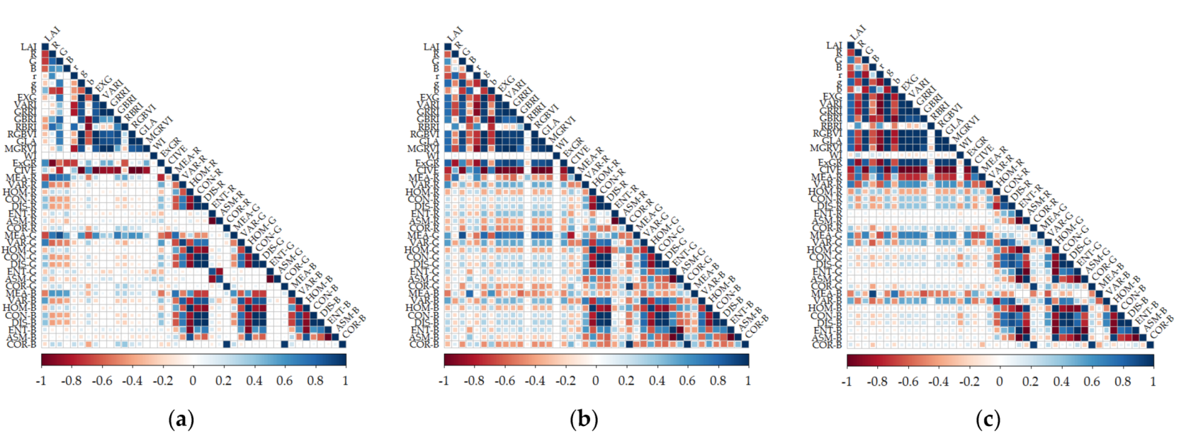
3.1. Correlation between LAI and UAV RGB Image Parameters

Correlation analysis was conducted between LAI of each growth period and 41 parameters which contained 17 spectral indices and 24 texture features constructed by UAV RGB images in the corresponding period, and then inversion variables that could continue to participate in this study were screened out. Because there were many selected research parameters, they were combined into variable sets according to the research method, and each variable set was named separately (Table 4). It can be seen from Figure 4 that 26 parameters at the initial flowering stage were highly significantly correlated with LAI (p < 0.01), and the absolute value of the correlation coefficient ranged from 0.291 to 0.713, with the highest correlation coefficient being R (−0.713). The variable set α was composed of 10 spectral features, and 16 texture features formed the variable set β in IF. In total, 35 parameters were highly significantly correlated (p < 0.01) with LAI at YF and FE, with the absolute value of the correlation coefficient in the range of 0.292–0.815, and the highest correlation was ExGR (0.815). Among them, 15 spectral features constituted the variable set γ, 20 texture features formed the variable set δ.

3.2. LAI Modeling and Accuracy Verification

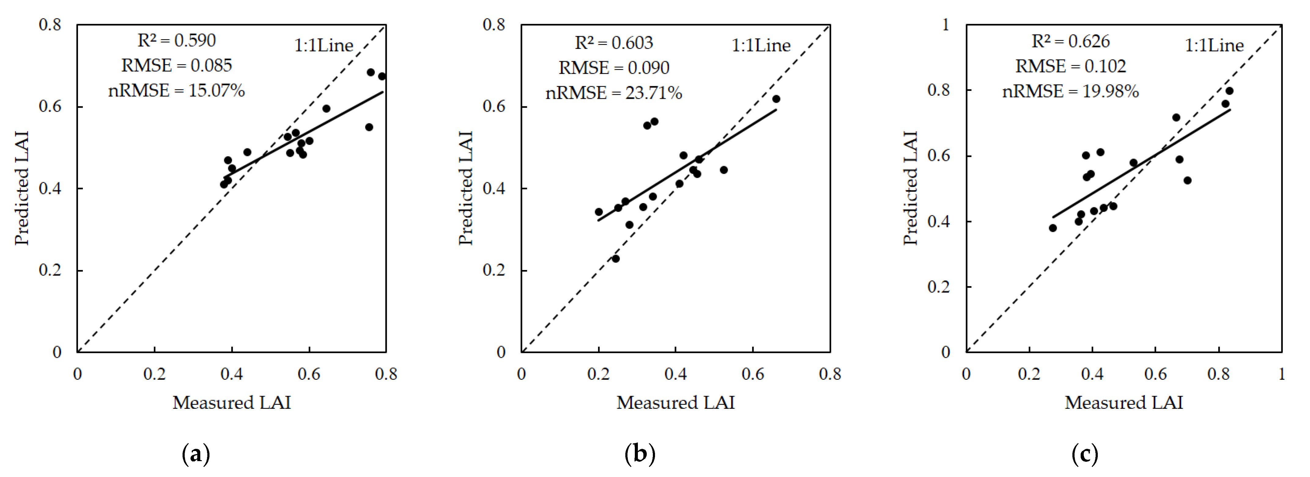
3.2.1. Unitary Linear Model Construction and Precision Analysis

According to the above correlation analysis results, the comparative analysis of LAI estimation models was conducted based on five single-factor and two multi-factor modeling methods. In single-factor modeling, the parameter with the highest correlation was selected as the independent variable in each period (Table S1), and five conventional functions were used for modeling. The model accuracy and other details were shown in Table 5. The fitting effect of quadratic polynomial function was the best in all growth stages, and the ability of prediction was general. In particular, R2 only reached 0.466 in IF, so the model should be prudently applied. In order to verify the applicability of the model, the validation set data were used to verify the model; moreover, fitting analysis was performed between the predicted and measured values. Figure 5 showed that in general the predicted value in the low value interval was lower than the measured value, while in the high value interval it was higher than the measured value. The precision of single-factor model was not preferable to model the monitoring LAI, so the multi-factor model needed to be established.

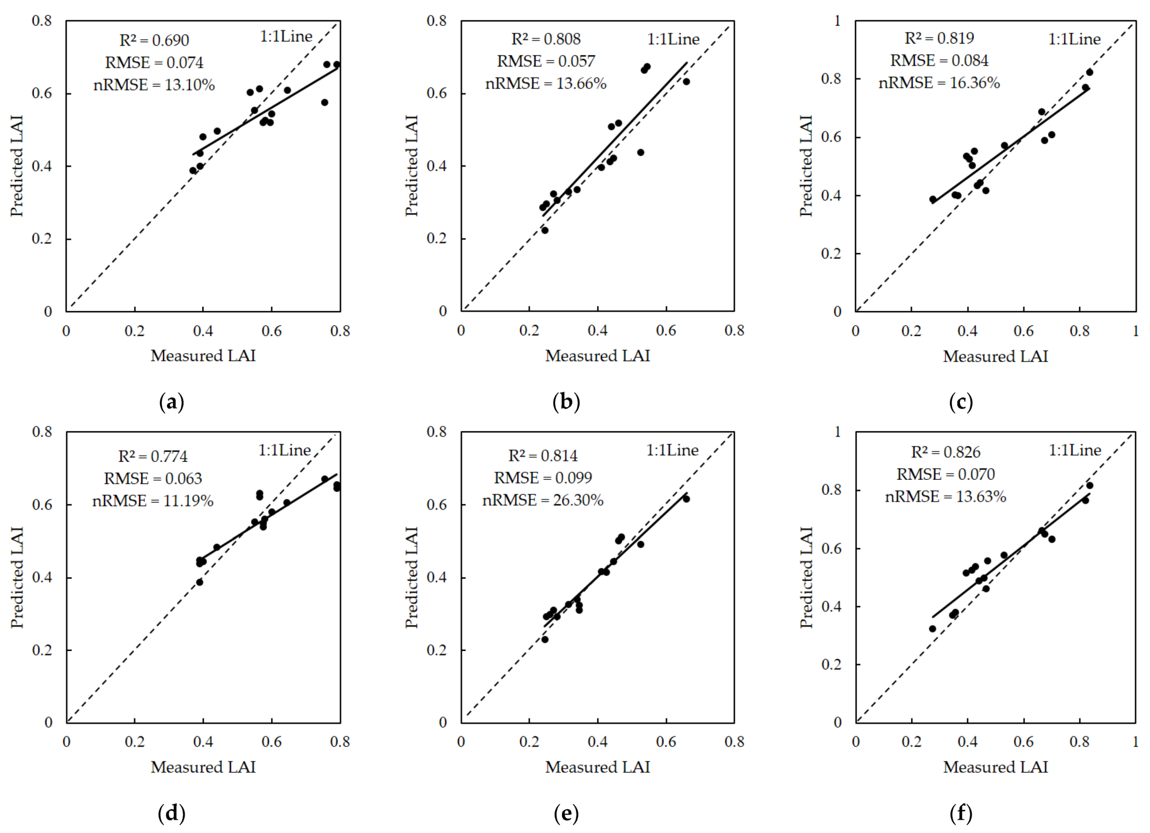
3.2.2. LAI Estimation Models Established by Spectral Index Only

The results in the SWR analysis are shown in Table S2. The combinations and quantities of spectral indices are diverse from each other in different growth stages. Iterated by the SWR model, the quantity of spectral indices was the most in YF with 9, followed by FE with 6 and IF with 3. The SWR analysis results indicated that the modeling R2 reached 0.541–0.819, and RMSE and nRMSE were 0.049–0.102 and 11.55–16.81% respectively (Table 6). In addition, verification R2 was 0.690–0.819, RMSE and nRMSE were 0.057–0.084 and 13.10–16.36%, separately (Figure 6). As seen here, there was a certain extent of improvement after adopting the SWR model in model accuracy at different growth stages. The analysis results of the RFR model showed that the modeling R2 of each period was greater than or equal to 0.965, with the highest reaching roughly 0.973. In terms of validation sets, the RFR model performed best at YF. Furthermore, the RFR model was consistently better performing than the SWR model at each growth stage.

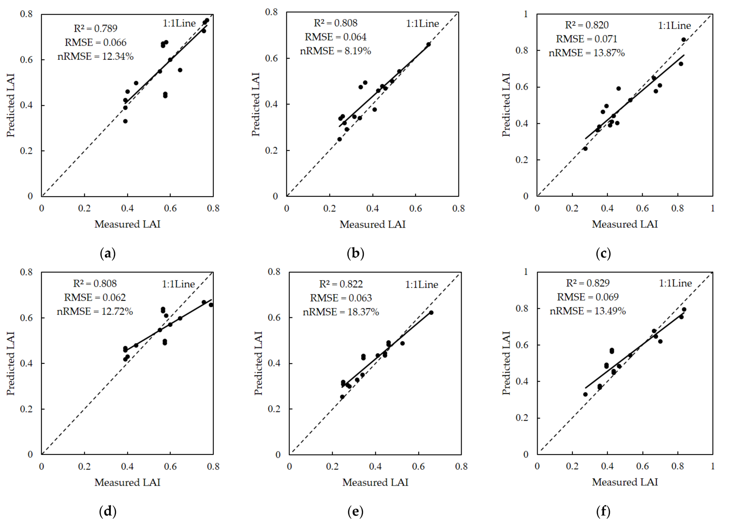
3.2.3. LAI Estimation Models Combined with Texture Features

The spectral indices and texture features were combined to construct LAI estimation models of kiwifruit based on the SWR and RFR algorithms respectively. The independent variable sets of the SWR model in Table 7 are the results screened by stepwise regression (Table S3) with the variables combining spectral indices and texture features. YF contains the most variables with 27, followed by FE with 21, and IF with 18. Due to the addition of texture information, the prediction accuracy of the two models was significantly improved at each growth stage. In particular, the SWR model performance of IF was significantly improved after combining the spectral indices and texture feature, with R2 increased by 0.318 to 0.859 at least; RMSE and nRMSE increased by 0.034 and 6.56% to 0.042 and 8.14%, respectively. Moreover, compared with the inversion only by the spectral index, the modeling R2 values of the RFR model with integrated texture features at each period were all greater than or equal to 0.968, and the RMSE and nRMSE were 0.032 and 5.30% at least. According to the validation results (Figure 7), the RFR model had the best performance in FE, and the R2, RMSE, and nRMSE were 0.829, 0.069, and 13.49%, respectively. Coincidentally, after combining the spectral indices and texture information the RFR model performed better than the SWR model at each period.

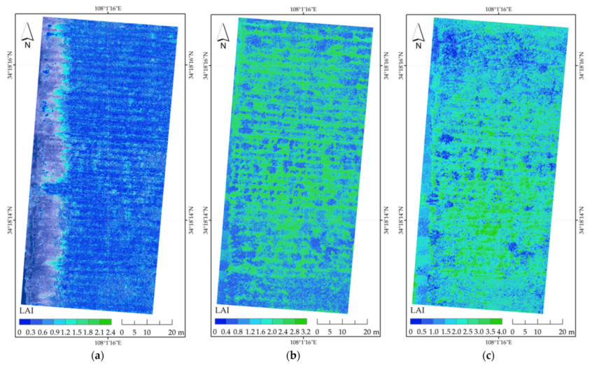
3.3. Model Selection and Inversion Mapping

From the perspective of the model accuracy, the RFR model with spectral indices combined with texture features was better for LAI estimation of kiwifruit in the study area at all growth stages. The image matrix for RGB bands and texture features in the three growth periods were respectively read and substituted into the optimal model, then the spatial distribution of LAI was symbolized by grading (Figure 8). It can be seen that in the initial flowering stage, the kiwifruit had just blossomed, and its leaves were small and sparse, so LAI was mostly less than 0.6 in the study area. At the young fruit stage, vines of kiwifruit benefited from sufficient rain and light and began to climb; their leaves piled up and staggered, so LAI generally ranged from 0 to 3.2. During the fruit enlargement stage, kiwifruit nutrition was provided for fruit accumulation. Although LAI was smaller in some areas than in the previous period, canopy leaves were also flourishing in most areas, with the overall LAI values ranging from 0 to 4.0.

4. Discussion

4.1. Feasibility of LAI Estimation by UAV RGB Images

Through the analysis of kiwifruit observation data in the study area and UAV RGB images obtained in three periods, it was proved that observed LAI was highly correlated with some spectral indices and texture information extracted from RGB and GLCM images to estimate LAI of kiwifruit. Nevertheless, on account of the diverse performance of these indices, it was complicated to establish general models between LAI and numerous spectral parameters. In particular, the unitary linear model was not recommended for LAI estimation of kiwifruit. On the contrary, the model based on machine learning algorithm performed well in estimating LAI, which could improve the estimation accuracy and reduce the workload [11,54]. In addition, the estimation accuracy established by the RFR model was satisfied for LAI estimation of kiwifruit at field scale. There have been many research results using UAV to monitor important crop growth parameters [7,55], such as chlorophyll content, nitrogen nutrient index, leaf area index, biomass, etc. Compared with the research results of many scholars, the feasibility of our results has been proved. Compared with the traditional LAI measurement method, this method illustrated the characteristics of nondestructive, convenient, and low-cost monitoring. Meanwhile, UAV can also realize a larger area of monitoring for kiwifruit LAI compared to the optical instrumentation method. As we all know, hyperspectral platforms contain many bands, resulting in complexity and redundancy in practical agricultural applications, the operation of which was more sophisticated [56]. The UAV platform with only three bands of red, green, and blue could also meet the accuracy requirements of kiwifruit growth recognition and monitoring; the operation was easier, and the application was less complicated in the actual environment. Thus, it had certain potential to estimate LAI of kiwifruit by UAV RGB images.

4.2. Advantages of Estimation after Combining with Texture Features

It was observed that the model accuracy of combining texture information was better than that of spectral index inversion only, for both the SWR or RFR models. The conclusion was consistent with that obtained by many scholars in the estimation of aboveground biomass of winter wheat and in diagnosis of winter-wheat water stress, etc. [12,33,37]. Because the spectral index integrating texture features includes both spectral and texture information of UAV images, it can essentially explain and construct kiwifruit growth from a two-dimensional perspective; therefore, the model accuracy is significantly improved. It is strongly suggested that more attention should be paid to the potential combination of texture features with spectral indices instead of the spectral indices only when analyzing agricultural-related applications [37]. At present, quantitative estimation of crop physiological and biochemical parameters is mainly focused on the selection of new vegetation indices, especially the combination of spectral parameters. Information extraction mainly relies on the spectral features of remote sensing images; however, remote sensing images are not limited to spectral features. All kinds of the spatial texture features of images are also important data sources of quantitative remote sensing. In addition, with the development of remote sensing in the future, it is hoped that more high-resolution meteorological satellite images will be added to enable further development of crop growth monitoring. In this study, the spectral indices extracted from the visible image were combined with the texture feature information of the image itself. In future studies, kiwifruit’s own state and environment parameters should be added into the estimation such as the height of the climbing above the pergola, mean daily temperature, mean daily solar radiation, etc., to demonstrate the model from the three or multiple dimensional perspectives in LAI estimation, so that it is possible to improve the accuracy of the model and simulate the growth situation of kiwifruit more closely.

4.3. Model Optimization Selection of LAI

In this paper, univariate and multivariable models were used to estimate LAI of kiwifruit. Among many univariate models, the accuracy of the quadratic polynomial model was relatively high, which was limited to making a simple prediction for young fruit stage and fruit enlargement stage, while the prediction accuracy of the model in the initial flowering stage was far from the inversion requirement. Compared with the univariate regression model, the inversion effects of multivariate model were improved significantly. This was relatively consistent with the current LAI estimation results of most crops [5,57,58], indicating that there was a certain quadratic polynomial fitting relationship between LAI and specific spectral indices. However, with the increase of variables, the multivariable model based on MLA was a better solution for LAI estimation. From the perspective of the differences between the two MLA models selected, this study concluded that, compared with the SWR model, the RFR model was more suitable for LAI estimation of kiwifruit. There have been various researchers exerting much effort in the area of crop growth modeling, who have concluded that stepwise regression is more suitable for the estimation of wheat crop phenology and crop yield [59,60]. Furthermore, the study of some researchers proved that random forest had advantages in estimating the chlorophyll content of apple leaves in the orchard [61]. The reason for the difference between the above conclusion and this study could be that there were some differences in crop growth trend and indices of estimation, and possibly also be related to crop varieties and growth period. Meanwhile, the mechanisms of the impacts of kiwifruit growth monitoring on machine learning should be further studied, because they always have an excellent performance in classification and regression. By using more advanced methods such as machine learning and deep learning involving multiple layers to identify crop growth, more extensible crop growth monitoring models will be selected. In this study, three representative growth periods of kiwifruit within one year were adopted to construct the model. In the selection of location and period, kiwifruit samples of diverse years and locations should be added in future investigations to obtain a more widely applicable estimation model. In addition, the values measured by CI-110 canopy analyzer were used as the calibration data of LAI in this study, which had the advantage of convenience and the measurement based on the characteristics of the optical instrument was more accurate and reliable in calibrating data. The measurement of LAI of kiwifruit by the CI-110 canopy analyzer is an extension of the study on orchard growth monitoring. However, additional instruments and methods should be used in the study of kiwifruit growth status as a supplement in follow-up studies.

5. Conclusions

In the investigation, spectral indices and texture features were extracted from UAV RGB images in the diverse kiwifruit growth period, and the LAI estimation model and spatial distribution were conducted by a series of new variable sets, constructing the single-factor and MLA models at the corresponding period. Notably, polytomy variables models with MLA performed well on estimating LAI, which could improve the estimation accuracy. In particular, a series of the new index sets combining spectral and textural information had achieved a higher precision when estimating the LAI, of which the validation R2 was 0.820 with SWR model in FE. Therefore, the new indices were suitable for the monitoring of kiwifruit growth model and it was strongly suggested that the spectral and textural information be combined in the growth monitoring of kiwi orchard. Furthermore, using the RFR model significantly improved the predictability and accuracy of the model according to the R2, RMSE, and nRMSE values. Verification results indicated that the prediction accuracy of models among the diverse growth stages was better when using the RFR model and the validation accuracy (R2 = 0.829) in FE was the best. In conclusion, the inversion technique with UAV combining spectral indices and texture features can provide a cost-effective, fast, and effective method for kiwifruit growth monitoring. Meanwhile, it can also realize the large-scale and high-quality monitoring of kiwifruit orchards, providing a theoretical basis for kiwi growth investigation.

Supplementary Materials

The following supporting information can be downloaded at: https://www.mdpi.com/article/10.3390/rs14051063/s1, Figure S1: Images taken and processed by CI-110; Figure S2: More images of parameters in the study; Table S1: Comparison of single-factor model for kiwifruit LAI in each growth stage; Table S2: Variable selection for SWR with only spectral indexes in each growth stage.

Author Contributions

Y.Z.: conceptualization, methodology, formal analysis, writing—original draft preparation, visualization. Q.C. (Qingrui Chang): conceptualization, funding acquisition, writing—review and editing. N.T.: conceptualization, resources, software. S.G.: resources, software. Q.C. (Qian Chen): resources, software. L.Z.: conceptualization, methodology. F.L.: funding acquisition. All authors have read and agreed to the published version of the manuscript.

Funding

This work was supported by the National Natural Science Foundation of China (NO. 41701398) and National High-tech R&D Program of China (863 Program) (NO. 2013AA102401-2).

Institutional Review Board Statement

Not applicable.

Informed Consent Statement

Not applicable.

Data Availability Statement

The experimental data were measured according to the test specifications, which can be used for further analysis.

Acknowledgments

The experimental data were measured according to the test specifications, which can be used for further analysis.

Conflicts of Interest

The authors declare no conflict of interest.

References

  1. Tian, Y.; Huang, H.; Zhou, G.; Zhang, Q.; Tao, J.; Zhang, Y.; Lin, J. Aboveground mangrove biomass estimation in Beibu Gulf using machine learning and UAV remote sensing. Sci. Total Environ. 2021, 781, 146816. [Google Scholar] [CrossRef]
  2. Kong, B.; Yu, H.; Du, R.; Wang, Q. Quantitative Estimation of Biomass of Alpine Grasslands Using Hyperspectral Remote Sensing. Rangel. Ecol. Manag. 2019, 72, 336–346. [Google Scholar] [CrossRef]
  3. Ali, A.; Imran, M. Evaluating the potential of red edge position (REP) of hyperspectral remote sensing data for real time estimation of LAI & chlorophyll content of kinnow mandarin (Citrus reticulata) fruit orchards. Sci. Hortic. 2020, 267, 109326. [Google Scholar] [CrossRef]
  4. Zhang, Y.; Hui, J.; Qin, Q.; Sun, Y.; Zhang, T.; Sun, H.; Li, M. Transfer-learning-based approach for leaf chlorophyll content estimation of winter wheat from hyperspectral data. Remote Sens. Environ. 2021, 267, 112724. [Google Scholar] [CrossRef]
  5. Gano, B.; Dembele, J.S.B.; Ndour, A.; Luquet, D.; Beurier, G.; Diouf, D.; Audebert, A. Using UAV Borne, Multi-Spectral Imaging for the Field Phenotyping of Shoot Biomass, Leaf Area Index and Height of West African Sorghum Varieties under Two Contrasted Water Conditions. Agronomy 2021, 11, 850. [Google Scholar]
  6. Zhang, J.; Li, M.; Sun, Z.; Liu, H.; Sun, H.; Yang, W. Chlorophyll Content Detection of Field Maize Using RGB-NIR Camera. IFAC-Paper 2018, 51, 700–705. [Google Scholar] [CrossRef]
  7. Bendig, J.; Bolten, A.; Bennertz, S.; Broscheit, J.; Eichfuss, S.; Bareth, G. Estimating Biomass of Barley Using Crop Surface Models (CSMs) Derived from UAV-Based RGB Imaging. Remote Sens. 2014, 6, 10395–10412. [Google Scholar]
  8. Wan, L.; Cen, H.; Zhu, J.; Zhang, J.; Zhu, Y.; Sun, D.; Du, X.; Zhai, L.; Weng, H.; Li, Y.; et al. Grain yield prediction of rice using multi-temporal UAV-based RGB and multispectral images and model transfer—Case study of small farmlands in the South of China. Agric. For. Meteorol. 2020, 291, 108096. [Google Scholar] [CrossRef]
  9. Li, B.; Xu, X.; Zhang, L.; Han, J.; Bian, C.; Li, G.; Liu, J.; Jin, L. Above-ground biomass estimation and yield prediction in potato by using UAV-based RGB and hyperspectral imaging. ISPRS J. Photogramm. Remote Sens. 2020, 162, 161–172. [Google Scholar] [CrossRef]
  10. Zheng, H.; Cheng, T.; Li, D.; Yao, X.; Tian, Y.; Cao, W.; Zhu, Y. Combining Unmanned Aerial Vehicle (UAV)-Based Multispectral Imagery and Ground-Based Hyperspectral Data for Plant Nitrogen Concentration Estimation in Rice. Front Plant Sci. 2018, 9, 936. [Google Scholar] [CrossRef]
  11. Qiu, Z.; Ma, F.; Li, Z.; Xu, X.; Ge, H.; Du, C. Estimation of nitrogen nutrition index in rice from UAV RGB images coupled with machine learning algorithms. Comput. Electron. Agric. 2021, 189, 106421. [Google Scholar] [CrossRef]
  12. Zhou, Y.; Lao, C.; Yang, Y.; Zhang, Z.; Chen, H.; Chen, Y.; Chen, J.; Ning, J.; Yang, N. Diagnosis of winter-wheat water stress based on UAV-borne multispectral image texture and vegetation indices. Agric. Water Manag. 2021, 256, 107076. [Google Scholar] [CrossRef]
  13. Lama, G.F.C.; Crimaldi, M.; Pasquino, V.; Padulano, R.; Chirico, G.B. Bulk Drag Predictions of Riparian Arundo donax Stands through UAV-Acquired Multispectral Images. Water 2021, 13, 1333. [Google Scholar]
  14. Taddia, Y.; Russo, P.; Lovo, S.; Pellegrinelli, A. Multispectral UAV monitoring of submerged seaweed in shallow water. Appl. Geomat. 2020, 12, 19–34. [Google Scholar] [CrossRef] [Green Version]
  15. Fernández-Lozano, J.; Sanz-Ablanedo, E. Unraveling the Morphological Constraints on Roman Gold Mining Hydraulic Infrastructure in NW Spain. A UAV-Derived Photogrammetric and Multispectral Approach. Remote Sens. 2021, 13, 291. [Google Scholar]
  16. Benos, L.; Tagarakis, A.C.; Dolias, G.; Berruto, R.; Kateris, D.; Bochtis, D. Machine Learning in Agriculture: A Comprehensive Updated Review. Sensors 2021, 21, 3758. [Google Scholar]
  17. Sadeghifar, T.; Lama, G.F.C.; Sihag, P.; Bayram, A.; Kisi, O. Wave height predictions in complex sea flows through soft-computing models: Case study of Persian Gulf. Ocean Eng. 2022, 245, 110467. [Google Scholar] [CrossRef]
  18. Hashim, W.; Eng, L.S.; Alkawsi, G.; Ismail, R.; Alkahtani, A.A.; Dzulkifly, S.; Baashar, Y.; Hussain, A. A Hybrid Vegetation Detection Framework: Integrating Vegetation Indices and Convolutional Neural Network. Symmetry 2021, 13, 2190. [Google Scholar]
  19. Watson, D.J. Comparative Physiological Studies on the Growth of Field Crops: I. Variation in Net Assimilation Rate and Leaf Area between Species and Varieties, and within and between Years. Ann. Bot. 1947, 11, 41–76. [Google Scholar]
  20. Negrón Juárez, R.I.; da Rocha, H.R.; e Figueira, A.M.S.; Goulden, M.L.; Miller, S.D. An improved estimate of leaf area index based on the histogram analysis of hemispherical photographs. Agric. For. Meteorol. 2009, 149, 920–928. [Google Scholar] [CrossRef] [Green Version]
  21. Vose, J.M.; Barton, D.; Clinton, N.H.; Sullivan, P.V.B. Vertical leaf area distribution, light transmittance, and application of the Beer–Lambert Law in four mature hardwood stands in the southern Appalachians. Can. J. For. Res. 1995, 25, 1036–1043. [Google Scholar]
  22. Wilhelm, W.W.; Ruwe, K.; Schlemmer, M.R. Comparison of three leaf area index meters in a corn canopy. Crop Sci. 2000, 40, 1179–1183. [Google Scholar]
  23. Glatthorn, J.; Pichler, V.; Hauck, M.; Leuschner, C. Effects of forest management on stand leaf area: Comparing beech production and primeval forests in Slovakia. For. Ecol. Manag. 2017, 389, 76–85. [Google Scholar] [CrossRef]
  24. Jiang, S.; Zhao, L.; Liang, C.; Hu, X.; Yaosheng, W.; Gong, D.; Zheng, S.; Huang, Y.; He, Q.; Cui, N. Leaf- and ecosystem-scale water use efficiency and their controlling factors of a kiwifruit orchard in the humid region of Southwest China. Agric. Water Manag. 2022, 260, 107329. [Google Scholar] [CrossRef]
  25. Srinet, R.; Nandy, S.; Patel, N.R. Estimating leaf area index and light extinction coefficient using Random Forest regression algorithm in a tropical moist deciduous forest, India. Ecol. Inform. 2019, 52, 94–102. [Google Scholar] [CrossRef]
  26. Ren, B.; Li, L.; Dong, S.; Liu, P.; Zhao, B.; Zhang, J. Photosynthetic Characteristics of Summer Maize Hybrids with Different Plant Heights. Agron. J. 2017, 109, 1454. [Google Scholar]
  27. Hassanijalilian, O.; Igathinathane, C.; Doetkott, C.; Bajwa, S.; Nowatzki, J.; Haji Esmaeili, S.A. Chlorophyll estimation in soybean leaves infield with smartphone digital imaging and machine learning. Comput. Electron. Agric. 2020, 174, 105433. [Google Scholar] [CrossRef]
  28. Lu, J.; Cheng, D.; Geng, C.; Zhang, Z.; Xiang, Y.; Hu, T. Combining plant height, canopy coverage and vegetation index from UAV-based RGB images to estimate leaf nitrogen concentration of summer maize. Biosyst. Eng. 2021, 202, 42–54. [Google Scholar] [CrossRef]
  29. Raj, R.; Walker, J.P.; Pingale, R.; Nandan, R.; Naik, B.; Jagarlapudi, A. Leaf area index estimation using top-of-canopy airborne RGB images. Int. J. Appl. Earth Obs. Geoinf. 2021, 96, 102282. [Google Scholar] [CrossRef]
  30. Shao, G.; Han, W.; Zhang, H.; Liu, S.; Wang, Y.; Zhang, L.; Cui, X. Mapping maize crop coefficient Kc using random forest algorithm based on leaf area index and UAV-based multispectral vegetation indices. Agric. Water Manag. 2021, 252, 106906. [Google Scholar] [CrossRef]
  31. Guo, Z.-c.; Wang, T.; Liu, S.-l.; Kang, W.-p.; Chen, X.; Feng, K.; Zhang, X.-q.; Zhi, Y. Biomass and vegetation coverage survey in the Mu Us sandy land-based on unmanned aerial vehicle RGB images. Int. J. Appl. Earth Obs. Geoinf. 2021, 94, 102239. [Google Scholar] [CrossRef]
  32. Li, Y.; Liu, H.; Ma, J.; Zhang, L. Estimation of leaf area index for winter wheat at early stages based on convolutional neural networks. Comput. Electron. Agric. 2021, 190, 106480. [Google Scholar] [CrossRef]
  33. Yue, J.; Yang, G.; Tian, Q.; Feng, H.; Xu, K.; Zhou, C. Estimate of winter-wheat above-ground biomass based on UAV ultrahigh-ground-resolution image textures and vegetation indices. ISPRS J. Photogramm. Remote Sens. 2019, 150, 226–244. [Google Scholar] [CrossRef]
  34. Flores, P.; Zhang, Z.; Igathinathane, C.; Jithin, M.; Naik, D.; Stenger, J.; Ransom, J.; Kiran, R. Distinguishing seedling volunteer corn from soybean through greenhouse color, color-infrared, and fused images using machine and deep learning. Ind. Crop. Prod. 2021, 161, 113223. [Google Scholar] [CrossRef]
  35. Waheed, A.; Goyal, M.; Gupta, D.; Khanna, A.; Hassanien, A.E.; Pandey, H.M. An optimized dense convolutional neural network model for disease recognition and classification in corn leaf. Comput. Electron. Agric. 2020, 175, 105456. [Google Scholar] [CrossRef]
  36. Maimaitijiang, M.; Sagan, V.; Sidike, P.; Maimaitiyiming, M.; Hartling, S.; Peterson, K.T.; Maw, M.J.W.; Shakoor, N.; Mockler, T.; Fritschi, F.B. Vegetation Index Weighted Canopy Volume Model (CVMVI) for soybean biomass estimation from Unmanned Aerial System-based RGB imagery. ISPRS J. Photogramm. Remote Sens. 2019, 151, 27–41. [Google Scholar] [CrossRef]
  37. Guo, Y.; Fu, Y.H.; Chen, S.; Robin Bryant, C.; Li, X.; Senthilnath, J.; Sun, H.; Wang, S.; Wu, Z.; de Beurs, K. Integrating spectral and textural information for identifying the tasseling date of summer maize using UAV based RGB images. Int. J. Appl. Earth Obs. Geoinf. 2021, 102, 102435. [Google Scholar] [CrossRef]
  38. Sumesh, K.C.; Ninsawat, S.; Som-ard, J. Integration of RGB-based vegetation index, crop surface model and object-based image analysis approach for sugarcane yield estimation using unmanned aerial vehicle. Comput. Electron. Agric. 2021, 180, 105903. [Google Scholar] [CrossRef]
  39. Haralick, R.M.; Shanmugam, K.; Dinstein, I. Textural Features for Image Classification. IEEE Trans. Syst. Man Cybern. 1973, SMC-3, 610–621. [Google Scholar]
  40. Laliberte, A.S.; Rango, A. Texture and Scale in Object-Based Analysis of Subdecimeter Resolution Unmanned Aerial Vehicle (UAV) Imagery. IEEE Trans. Geosci. Remote Sens. 2009, 47, 761–770. [Google Scholar]
  41. Murray, H.; Lucieer, A.; Williams, R. Texture-based classification of sub-Antarctic vegetation communities on Heard Island. Int. J. Appl. Earth Obs. Geoinf. 2010, 12, 138–149. [Google Scholar]
  42. Kelsey, K.C.; Neff, J.C. Estimates of Aboveground Biomass from Texture Analysis of Landsat Imagery. Remote Sens. 2014, 6, 6407–6422. [Google Scholar]
  43. Sarker, L.R.; Nichol, J.E. Improved forest biomass estimates using ALOS AVNIR-2 texture indices. Remote Sens. Environ. 2011, 115, 968–977. [Google Scholar]
  44. Chen, J.M.; Cihlar, J. Retrieving leaf area index of boreal conifer forests using Landsat TM images. Remote Sens. Environ. 1996, 55, 153–162. [Google Scholar] [CrossRef]
  45. Torres-Sánchez, J.; Pena, J.M.; De Castro, A.I.; López-Granados, F. Multi-temporal mapping of the vegetation fraction in early-season wheat fields using images from UAV. Comput. Electron. Agric. 2014, 103, 104–113. [Google Scholar]
  46. Soudani, K.; Fran?Ois, C.; Maire, G.L.; Dantec, V.L.; Dufrêne, E. Comparative analysis of IKONOS, SPOT, and ETM+ data for leaf area index estimation in temperate coniferous and deciduous forest stands. Remote Sens. Environ. 2006, 102, 161–175. [Google Scholar]
  47. Verrelst, J.; Schaepman, M.E.; Koetz, B.; Kneubühler, M. Angular sensitivity analysis of vegetation indices derived from CHRIS/PROBA data. Remote Sens. Environ. 2008, 112, 2341–2353. [Google Scholar]
  48. Sellaro, R.; Crepy, M.; Trupkin, S.A.; Karayekov, E.; Buchovsky, A.S.; Rossi, C.; Casal, J.J. Cryptochrome as a Sensor of the Blue/Green Ratio of Natural Radiation in Arabidopsis. Plant Physiol. 2010, 154, 401–409. [Google Scholar]
  49. Bendig, J.; Yu, K.; Aasen, H.; Bolten, A.; Bennertz, S.; Broscheit, J.; Gnyp, M.L.; Bareth, G. Combining UAV-based plant height from crop surface models, visible, and near infrared vegetation indices for biomass monitoring in barley. Int. J. Appl. Earth Obs. Geoinf. 2015, 39, 79–87. [Google Scholar] [CrossRef]
  50. Zhang, J.; Tian, H.; Wang, D.; Li, H.; Mouazen, A.M. A novel spectral index for estimation of relative chlorophyll content of sugar beet. Comput. Electron. Agric. 2021, 184, 106088. [Google Scholar] [CrossRef]
  51. Wu, J.; Wang, D.; Bauer, M.E. Assessing broadband vegetation indices and QuickBird data in estimating leaf area index of corn and potato canopies. Field Crop. Res. 2007, 102, 33–42. [Google Scholar] [CrossRef]
  52. Meyer, G.E.; Neto, J.C. Verification of color vegetation indices for automated crop imaging applications. Comput. Electron. Agric. 2008, 63, 282–293. [Google Scholar] [CrossRef]
  53. Li, H.; Chen, Z.-x.; Jiang, Z.-w.; Wu, W.-b.; Ren, J.-q.; Liu, B.; Tuya, H. Comparative analysis of GF-1, HJ-1, and Landsat-8 data for estimating the leaf area index of winter wheat. J. Integr. Agric. 2017, 16, 266–285. [Google Scholar] [CrossRef]
  54. Singh, A.; Ganapathysubramanian, B.; Singh, A.K.; Sarkar, S. Machine Learning for High-Throughput Stress Phenotyping in Plants. Trends Plant Sci. 2016, 21, 110–124. [Google Scholar] [CrossRef] [Green Version]
  55. Cen, H.; Wan, L.; Zhu, J.; Li, Y.; Li, X.; Zhu, Y.; Weng, H.; Wu, W.; Yin, W.; Xu, C.; et al. Dynamic monitoring of biomass of rice under different nitrogen treatments using a lightweight UAV with dual image-frame snapshot cameras. Plant Methods 2019, 15, 32. [Google Scholar] [CrossRef]
  56. Geipel, J.; Link, J.; Claupein, W. Combined Spectral and Spatial Modeling of Corn Yield Based on Aerial Images and Crop Surface Models Acquired with an Unmanned Aircraft System. Remote Sens. 2014, 6, 10335–10355. [Google Scholar]
  57. Yamaguchi, T.; Tanaka, Y.; Imachi, Y.; Yamashita, M.; Katsura, K. Feasibility of Combining Deep Learning and RGB Images Obtained by Unmanned Aerial Vehicle for Leaf Area Index Estimation in Rice. Remote Sens. 2021, 13, 84. [Google Scholar]
  58. Sun, B.; Wang, C.; Yang, C.; Xu, B.; Zhou, G.; Li, X.; Xie, J.; Xu, S.; Liu, B.; Xie, T.; et al. Retrieval of rapeseed leaf area index using the PROSAIL model with canopy coverage derived from UAV images as a correction parameter. Int. J. Appl. Earth Obs. Geoinf. 2021, 102, 102373. [Google Scholar] [CrossRef]
  59. Adnan, M.; Abaid-ur-Rehman, M.; Latif, M.A.; Ahmad, N.; Akhter, N. Mapping wheat crop phenology and the yield using machine learning (ML). Int. J. Adv. Comput. Sci. Appl. 2018, 9, 301–306. [Google Scholar]
  60. Liu, Y.; Heuvelink, G.B.M.; Bai, Z.; He, P.; Xu, X.; Ding, W.; Huang, S. Analysis of spatio-temporal variation of crop yield in China using stepwise multiple linear regression. Field Crop. Res. 2021, 264, 108098. [Google Scholar] [CrossRef]
  61. Ta, N.; Chang, Q.; Zhang, Y. Estimation of Apple Tree Leaf Chlorophyll Content Based on Machine Learning Methods. Remote Sens. 2021, 13, 3902. [Google Scholar] [CrossRef]
Figure 1. Geographic location and observation points of the study area.
Remotesensing 14 01063 g001
Figure 2. Three-dimensional visualization of sampling sites and equipment in the kiwifruit orchard.
Remotesensing 14 01063 g002
Figure 3. Part of the parameters analyzed in the study. (a) R (DN value of Red Channel) (IF); (b) MGRVI (Modified Green Red Vegetation Index); (c). MEA_R (the mean of the red band).
Remotesensing 14 01063 g003
Figure 4. Correlation between UAV image characteristic parameters and LAI at different growth stages. (a) Initial flowering stage (IF); (b) young fruit stage (YF); (c) fruit enlargement stage (FE).
Remotesensing 14 01063 g004
Figure 5. Validation results of single-factor model for kiwifruit LAI in each growth stage. (a) Initial flowering stage (IF); (b) young fruit stage (YF); (c) fruit enlargement stage (FE).
Remotesensing 14 01063 g005
Figure 6. Validation results of spectral parameters model for SWR and RFR models in each growth stage. (a) With SWR model in initial flowering stage (IF); (b) with SWR model in young fruit stage (YF); (c) with SWR model in fruit enlargement stage (FE); (d) with RFR model in initial flowering stage (IF); (e) with RFR model in young fruit stage (YF); (f) with RFR model in fruit enlargement stage (FE).
Remotesensing 14 01063 g006
Figure 7. Validation results of combined texture feature models with SWR and RFR in each growth stage. (a) With SWR model in initial flowering stage (IF); (b) with SWR model in young fruit stage (YF); (c) with SWR model in fruit enlargement stage (FE); (d) with RFR model in initial flowering stage (IF); (e) with RFR model in young fruit stage (YF); (f) with RFR model in fruit enlargement stage (FE).
Remotesensing 14 01063 g007
Figure 8. Spatial distribution of kiwifruit LAI estimation in study area. (a) Initial flowering stage (IF); (b) young fruit stage (YF); (c) fruit enlargement stage (FE).
Remotesensing 14 01063 g008
Table 1. Image information obtained by UAV.
Growth StagesDateNumber of Images
Initial flowering stage (IF)8 May145
Young fruit stage (YF)5 June144
Fruit enlargement stage (FE)8 July146
Table 2. Spectral parameters related to LAI of UAV RGB images.
ParametersNameFormulasSources
RDN value of Red Channel R = DN R Conventional empirical parameters
GDN value of Green Channel G = DN G
BDN value of Blue Channel B = DN B
rNormalized Redness Intensity r = R / ( R + G + B )
gNormalized Greenness Intensity g = G / ( R + G + B )
bNormalized Blueness Intensity b = B / ( R + G + B )
EXGExcess Green Index EXG = 2 × R G + B [45]
VARIVisible Atmospherically
Resistant Index
VARI = ( R + G ) / ( R + G B ) [46]
GRRIGreen Red Ratio Index GRRI = G   /   R [47]
GBRIGreen Blue Ratio Index GBRI = G   /   B [48]
RBRIRed Blue Ratio Index RBRI = R   /   B [48]
RGBVIRed Green Blue Vegetation Index RGBVI = ( G 2 BR )   /   ( G 2 + BR ) [49]
GLAGreen Leaf Algorithm GLA = ( 2 G R B )   /   ( 2 G + R + B ) [50]
MGRVIModified Green
Red Vegetation Index
MGRVI = ( G 2 R 2 )   /   ( G 2 + R 2 ) [49]
WIWoebbecke Index WI = ( G B )   /   ( R G ) [51]
ExGRExcess Green Red Index ExGR = ExG 1.4 R G [52]
CIVEColor Index of Vegetation CIVE = 0.441 R 0.881 G + 0.385 B + 18.78745 [53]
Table 3. Textural parameters related to LAI of UAV RGB images.
ParametersNameFormulasSources
MEAMean MEA i = i , j = 0 n 1 i ( P i , , j ) ,
MEA j = i , j = 0 n 1 j ( P i , , j )
[39]
VARVariance VAR i = i , j = 0 n 1 P i , , j ( i MEA i ) 2
VAR j = i , j = 0 n 1 P i , , j ( j MEA j ) 2
HOMHomogeneity HOM = i , j = 0 n 1 A i , j 1 + ( i j ) 2
CONContrast CON = i , j = 0 n 1 A i , j ( i j i ) 2
DISDissimilarity DIS = i , j = 0 n 1 A i , j | i j |
ENTEntropy ENT = i , j = 0 n 1 A ( i , j ) logA ( i , j )
ASMAngular Second Moment CON = i , j = 0 n 1 A i , j 2
CORCorrelation HOM = i , j = 0 n 1 P i , , j ( i MEA i ) ( j MEA j ) VAR i 2 VAR j 2
Table 4. The set of variables used in the study.
Set
Name
VariablesMethods for
Combination
αR, G, ExGR, B, b, RBRI, GBRI,
CIVE, EXG, RGBVI
Spectral indices highly
correlated with LAI in IF
βVAR_G, VAR_R, MEA_R, MEA_G,
VAR_B, MEA_B, CON_R, CON_G,
CON_B, DIS_R, DIS_G, DIS_B,
HOM_B, HOM_R, HOM_G, ASM_G
Texture features highly
correlated with LAI in IF
γR, G, B, r, g, b, EXG, VARI, GRRI, GBRI,
RGBVI, GLA, MGRVI, ExGR, CIVE
Spectral indices highly
correlated with LAI in YF and FE
δMEA_R, VAR_R, HOM_R, DIS_R, ENT_R,
ASM_R, COR_R, MEA_G, VAR_G, HOM_G,
DIS_G, ENT_G, COR_G, MEA_B, VAR_B,
HOM_B, DIS_B, ENT_B, ASM_B, COR_B
Texture features highly
correlated with LAI in YF and FE
Note: High correlation is defined as significance level of p < 0.01.
Table 5. Comparison of single-factor model for kiwifruit LAI in each growth stage.
Growth
Stages
Independent
Variable
Modeling EquationR2RMSEnRMSE/%
IFRy = 0.0005x2 − 0.1028x + 5.28730.4660.08115.86
YFExGRy = −0.00001784x2 + 0.00006079x + 1.0040.7190.06114.22
FEExGRy = 0.00006931x2 + 0.03275x + 4.2150.7360.10817.84
Table 6. Comparison of SWR and RFR analyses for spectral parameters in each growth stage.
Growth StagesModeling MethodSpectral
Parameters
AICR2RMSEnRMSE/%
IFSWRG, b, GBRI−323.230.5410.07514.70
RFRα-0.9650.0214.05
YFSWRR, G, r, g, VARI, GRRI, GBRI, RGBVI, GLA−365.100.8190.04911.55
RFRγ-0.9730.0194.42
FESWRR, G, g, GRRI, GBRI, MGRVI−278.640.7650.10216.81
RFRγ-0.9720.0355.80
Table 7. Comparison of SWR and RFR analyses for combined texture features in each growth stage.
Growth StagesModeling MethodSpectral
Parameters
AICR2RMSEnRMSE/%
IFSWRR, G, B, b, GBRI, RBRI, RGBVI, VAR_R, HOM_R, CON_R, DIS_R, MEA_G, VAR_G, ASM_G, VAR_B, HOM_B, CON_B, DIS_B−368.880.8590.0428.14
RFRα + β-0.9680.0203.88
YFSWRR, G, B, g, VARI, GRRI, GBRI, RGBVI, GLA, MGRVI, MEA_R, VAR_R, DIS_R, ENT_R, ASM_R, COR_R, VAR_G, HOM_G, DIS_G, ENT_G, COR_G, MEA_B, VAR_B, HOM_B, DIS_B, ENT_B, ASM_B−465.040.9780.0173.99
RFRγ + δ-0.9780.0174.08
FESWRR, B, r, g, VAAI, GRRI, GBRI, RGBVI, GLA, MGRVI, VAR_R, ENT_R, COR_R, MEA_G, HOM_G, ENT_G, COR_G, MEA_B, HOM_B, ENT_B, ASM_B−343.920.9470.0487.99
RFRγ + δ-0.9770.0325.30
Publisher’s Note: MDPI stays neutral with regard to jurisdictional claims in published maps and institutional affiliations.

