
Exploratory Analysis on Pixelwise Image Segmentation Metrics with an Application in Proximal Sensing

 ,
,  , , and
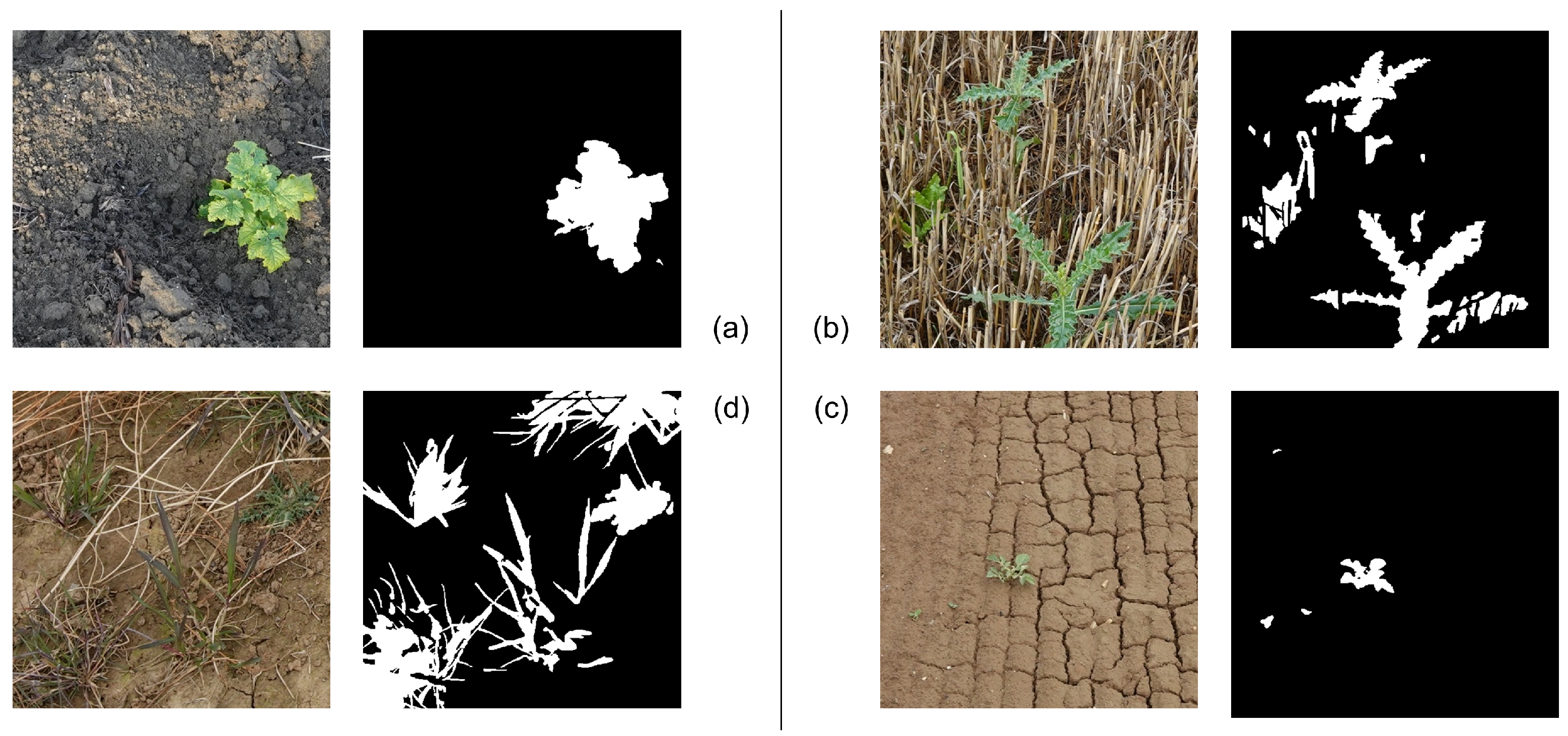
Abstract
:1. Introduction
- Provide a unified presentation of multiple pixel-level evaluation metrics for image segmentation;
- Define and develop a valid data mining exploratory approach that is both statistically valid and easily interpretable for the study of the relationships among these metrics;
- Provide a typological interpretation of the identified groups of metrics based on the observable segmentation results, with the aim of helping practitioners identify the useful metrics for their application.
2. Materials and Methods
2.1. Experimental Dataset of Plant Images
2.2. Three Segmentation Models for Experimentation
2.2.1. Decision Tree Segmentation Model
2.2.2. Support Vector Segmentation Machine
- Transform the pixels from the original RGB colour space to the CIELuv colour space;
- Train the SVM on the extracted features.
2.2.3. Colour Index of Vegetation Extraction
2.3. Metrics
2.3.1. Overlap Cardinalities
| Prediction | ||||
| Total | ||||
| GT | TP | FN | P | |
| FP | TN | N | ||
| Total | n | |||
2.3.2. Definition of the Metrics
- Positive predictive value: Precision (PRC)This metric is the proportion of pixels actually labelled as plant among all the pixels predicted as plant. It allows us to see the precision of the model in predicting plant pixels.
- Negative Predictive Value (NPV)This metric shows the proportion of pixels correctly classified as background among all the pixels classified as background. This allows us to see the precision of the algorithm on the background pixels.
- Recall (RCL)Known also as the true positive rate, this is the proportion of pixels correctly classified as plant among all the pixels that are in reality plant pixels.
- -Score (F1S)This metric combines precision and recall into one evaluation metric parameterised by , which specifies how much more we are interested in the recall than in the precision [29]. Formally, the -score is defined as:The most common version used is the -score, which assigns the same importance to precision and recall with :
- Accuracy (ACC)Probably one of the most widely used evaluation metrics for classification problems, this quantity shows the proportion of correct decisions among all decisions made, that is the proportion of pixels correctly classified, among all the pixels in the image:
- Balanced Accuracy (BAC)Introduced in [4] with the aim of solving the problem faced by the accuracy, the balanced accuracy can be defined as:where . In this case, we define c as the cost associated with the misclassification of a positive example, which gives us the freedom to set the penalisation in the case of misclassification on our class of interest. This may prove to be extremely important in certain use cases where there is a considerable loss associated with the misclassification of positive cases. In this work, we take in order to give equal weights to the two classes;
- Intersection Over Union (Jaccard Index) (IOU)Widely used in the computer vision literature on a variety of vision tasks including object detection and image segmentation, the Intersection over Union (IoU)—also known as the Jaccard Index—is perhaps the most famous spatial overlap metric in usage. For two finite sets A and B, it can be defined as:where is the set cardinality operator. Taking the two sets of interest to be our ground truth and detection masks, we can measure their similarity as:It was shown in [20] that in the case of binary classification, where the two sets studied are the sets of elements being classified (in our case, the pixels), the Jaccard Index can be easily reformulated in terms of the overlap cardinalities as:
- Global Consistency Error (GCE)The GCE [30] is a global measure of the segmentation error between two segmentation masks, based on the aggregation of local consistency errors measured at each pixel. Being a measure of error, it is a metric to be minimised. Defining as the set of all pixels that belong to the same class as the pixel p in the segmentation M, then we can define the segmentation error between two segmentations M and at p as:where \ is the set difference operator. As such, the GCE is defined as the error averaged over all the pixels and given by:
- Relative Vegetation Area (RVA)This metric, specific to the case of binary segmentation and proposed in [31], is a simple spatial overlap metric, which compares the area of vegetation detected in the segmentation mask to the true detection area in the ground truth mask. It is defined as:where is the vegetation area (number of plant pixels) in the ground truth mask and is the vegetation area in the detection mask;
- Adjusted Mutual Information Index (AMI)The mutual information of two random variables X and Y is a quantification of the amount of information that X holds about Y. It measures the reduction in uncertainty about Y given knowledge of X. The mutual information index of two segmentation masks M and can be understood as a measure of the amount of true information that the detection mask produced by the algorithm contains, in comparison to the information contained in the GT mask. It is based on the marginal entropies , and the joint entropy , which are defined as:where is the probability of observing a pixel of class i in the mask M, which can be expressed in terms of the four overlap cardinalities as:and the joint probabilities as:and finally, the Mutual Information Index (MI) is defined as:
- Cohen’s Kappa Coefficient (KAP)On the probabilistic side, we implemented Cohen’s Kappa coefficient, which is a measure of agreement between two samples. As an advantage over other measures with the exception of the AMI, the Kappa takes into account the agreement caused by chance, thus making it a fairer measure of model performance. It can be defined as:where “ is the agreement between the two samples” (simply, ACC), and “ is the hypothetical probability of chance agreement” [20]. We can re-write the Kappa using frequencies, which in turn can be expressed using the four overlap cardinalities, in order to facilitate our computations:
- Hausdorff Distance (HDD)Originally, this metric was formulated to measure the dissimilarity between two subsets of a metric space [34]. Informally, it allows measuring the degree of mismatch between two finite sets by measuring the distance from the point of Set 1 that is farthest from any point of Set 2, and vice versa. For example, if the distance between the two sets is k, then every point in one set must be within a distance k from every point in the other set [35]. This metric has been previously introduced and widely applied in the computer vision literature, especially in the field of medical imagery [20,35].Formally, for two finite sets M and , we define the Hausdorff distance as:where and d is some distance metric, which is usually, and in our case, the Euclidean distance.The closer the two objects M and are to each other in the Hausdorff distance, the more similar they are in shape. That is, two segmentation masks that have a low Hausdorff distance are masks in which the pixels are similarly distributed spatially over the grid. A more detailed formulation about the computation of the Hausdorff distance for comparing images can be found in [35].
2.4. Methodology for the Exploration of Metrics’ Relationships
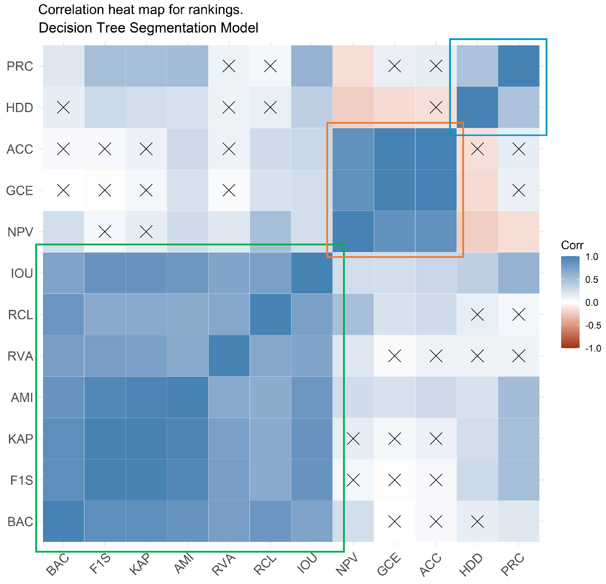
- Correlation analysisThe first analysis conducted was the study of the correlation matrix computed based on Spearman’s rank correlation. Spearman’s correlation is a well-known nonparametric measure of rank correlation, showing how well the relationship between two variables can be described using a monotonic function, regardless of whether this relationship is linear or not [37]. It is clear that Spearman’s correlation is simply the Pearson correlation applied to the rank variables. In our case, two metrics that have a high Spearman correlation are thus consistently ranking the same image similarly, as a good-quality image with a high ranking in the dataset, or otherwise. As such, it can be seen as a measure of “agreement” between the metrics;
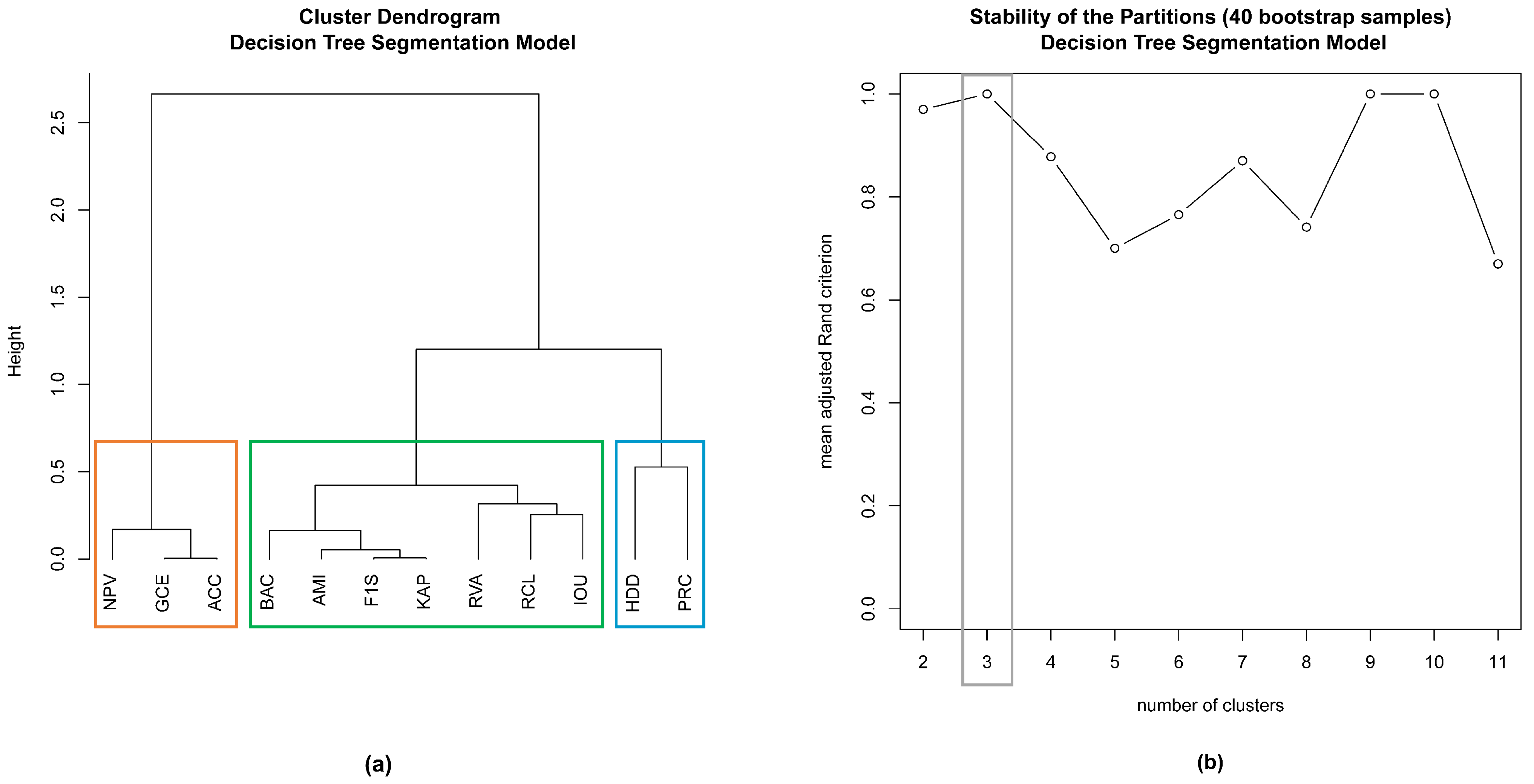
- Clustering of variablesAnother elaborate method for the exploration of relationships among variables is clustering of variables [38]. This method provides results that are clear to understand, interpret, visualise, and report. Given a set of quantitative variables, the aim of this method is to find the partition of these variables into K clusters in such a way so as to maximise the “homogeneity” of the partition, which indeed amounts to maximising the correlations among the variables of the same cluster. The clustering method used was hierarchical clustering, aiming at building a set of p nested partitions of variables following the algorithm detailed in [38]. This method was implemented in R using the package ClustOfVar [38];
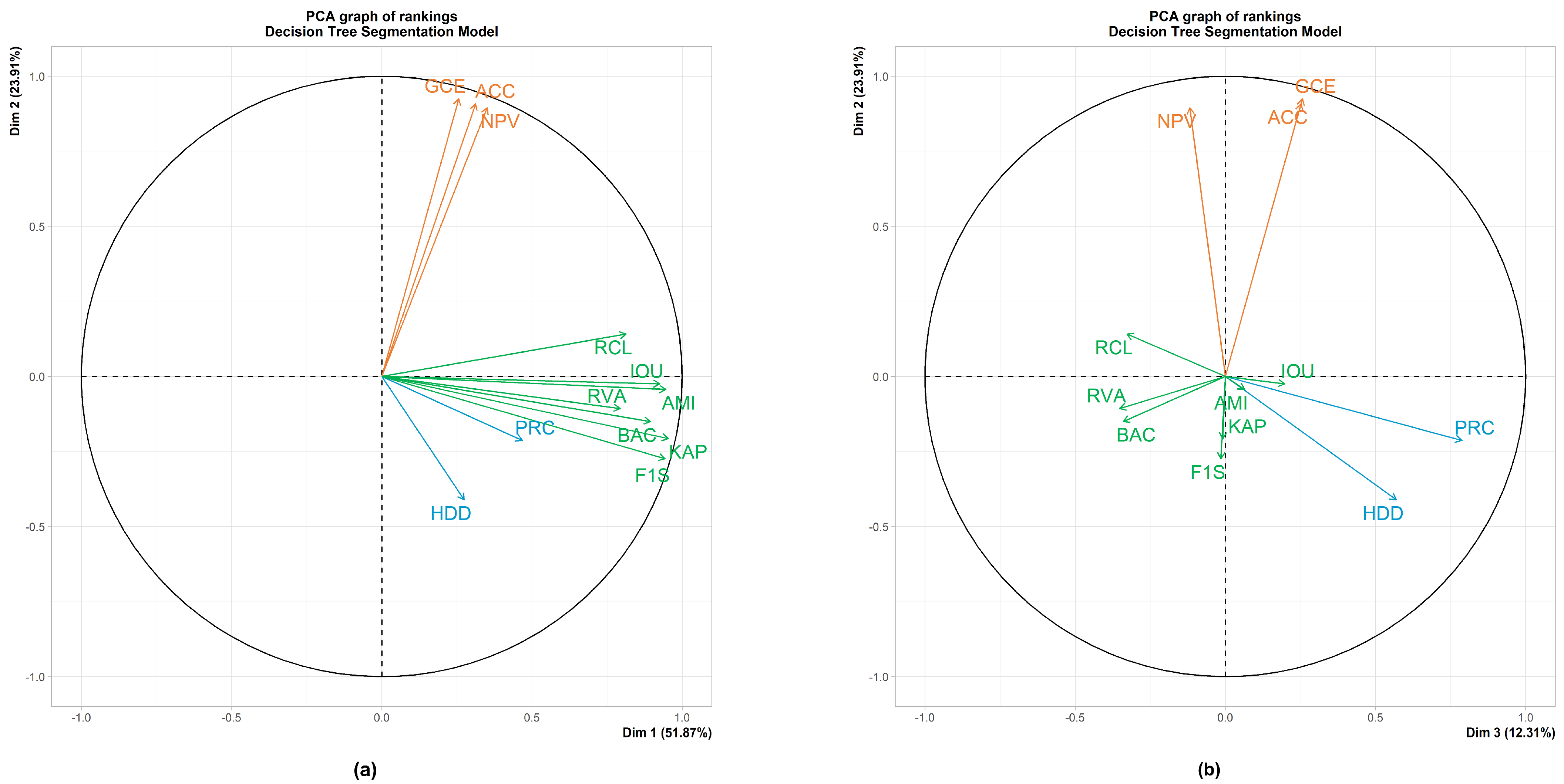
- Principal Component Analysis (PCA)To further confirm our results and to provide a clearer visualisation of the results, we conducted a Principal Component Analysis (PCA) [39,40] and plotted the obtained correlation circles. PCA aims at constructing new variables that are linear combinations of the original ones, under the constraints that all Principal Components (PCs) be pairwise orthogonal, with the first PC explaining the largest part of the dataset’s inertia, that is having the greatest “explicative” power, the second PC having the second largest inertia, and so on. The correlation circle that shows the projection in 2D of the variables with respect to some chosen PCs is a well-known and easily interpretable result of PCA, which allows us to visually identify groups of highly correlated variables among each other, and with particular PCs. This analysis was conducted in R using the package FactoMineR [41];
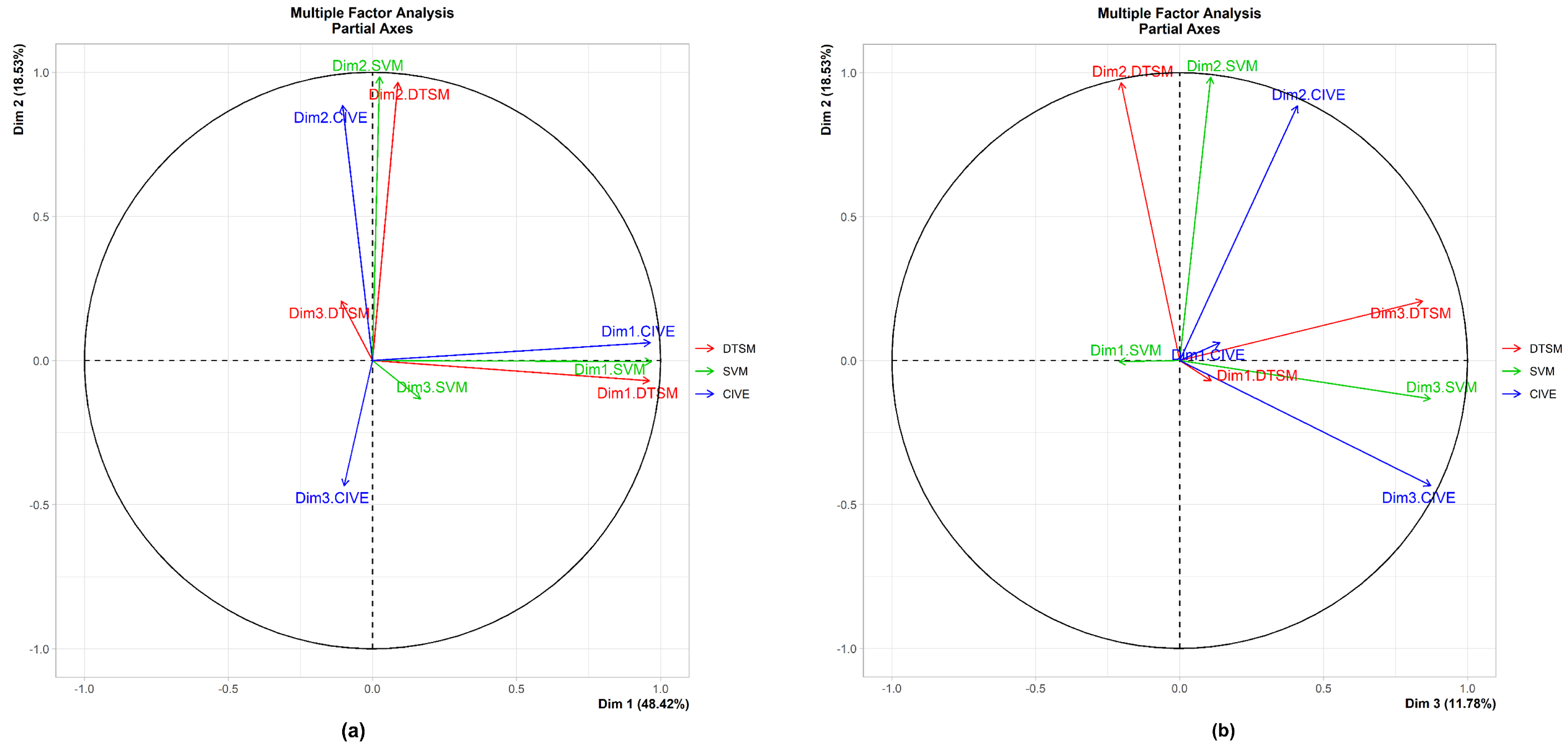
- Multiple factor analysisIn Section 3.1.1 and Section 3.1.2, the results of the three exploratory methods are shown only for the decision tree segmentation model, for conciseness. However, in order to verify that the results we obtained were not model dependent, we applied a Multiple Factor Analysis (MFA) [42,43] on the rankings produced by the three models. The result of this analysis would show us whether the relationships among the metrics differ largely from one model to another, or otherwise. From a simple perspective, the MFA can be understood as a PCA applied on the principal components obtained by the separate PCAs for each model, although the method is more elaborate. The most valuable result produced by MFA for this study was the representation of the partial axes. It consists of visualising the projection of the first and second dimensions obtained in each separate group PCA, on the principal plane of the MFA, formed by the first and second principal vectors of the MFA [42]. Such a method allows visualising how well correlated each of the most important dimensions of each group are with their respective global ones, in addition to showing their correlation among each other. The MFA was implemented in R using the package FactoMineR [41].
3. Results
3.1. Results of the Analysis on One Model
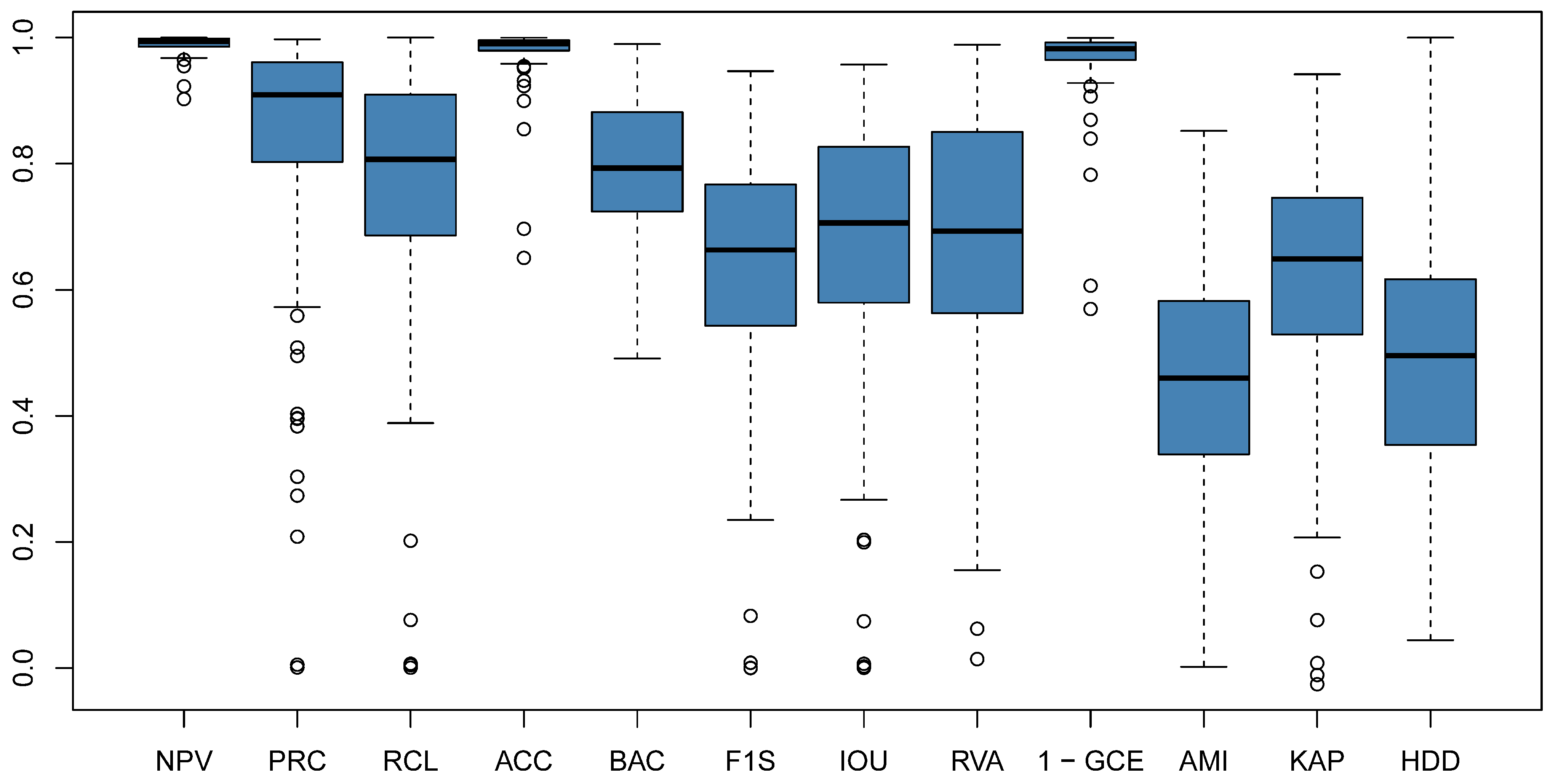
3.1.1. Correlation Analysis
3.1.2. Clustering of Variables
3.1.3. Principal Component Analysis
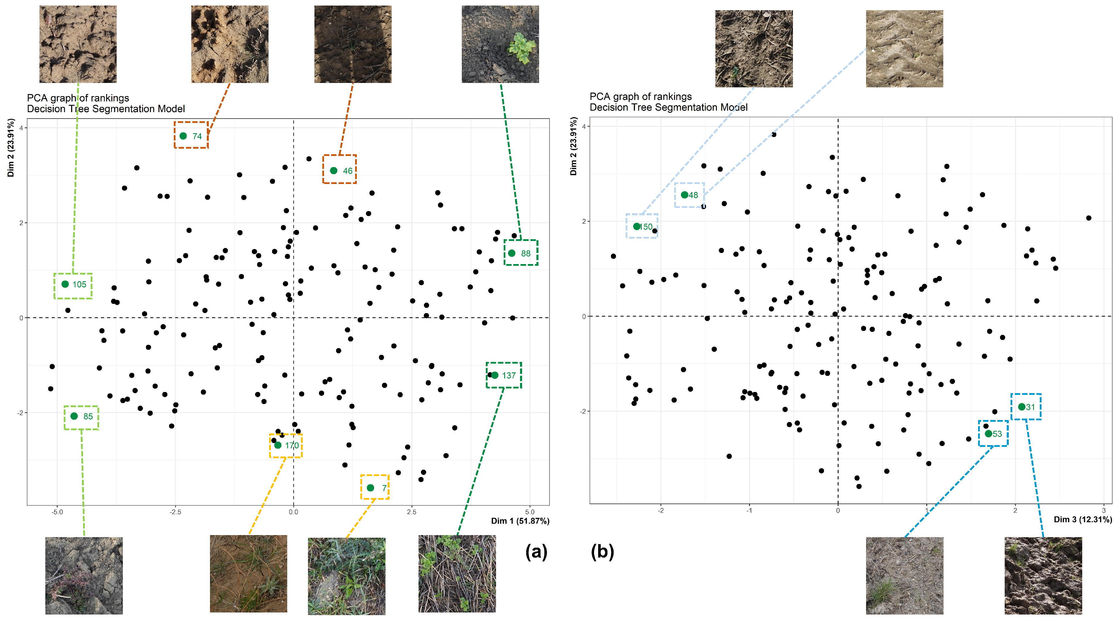
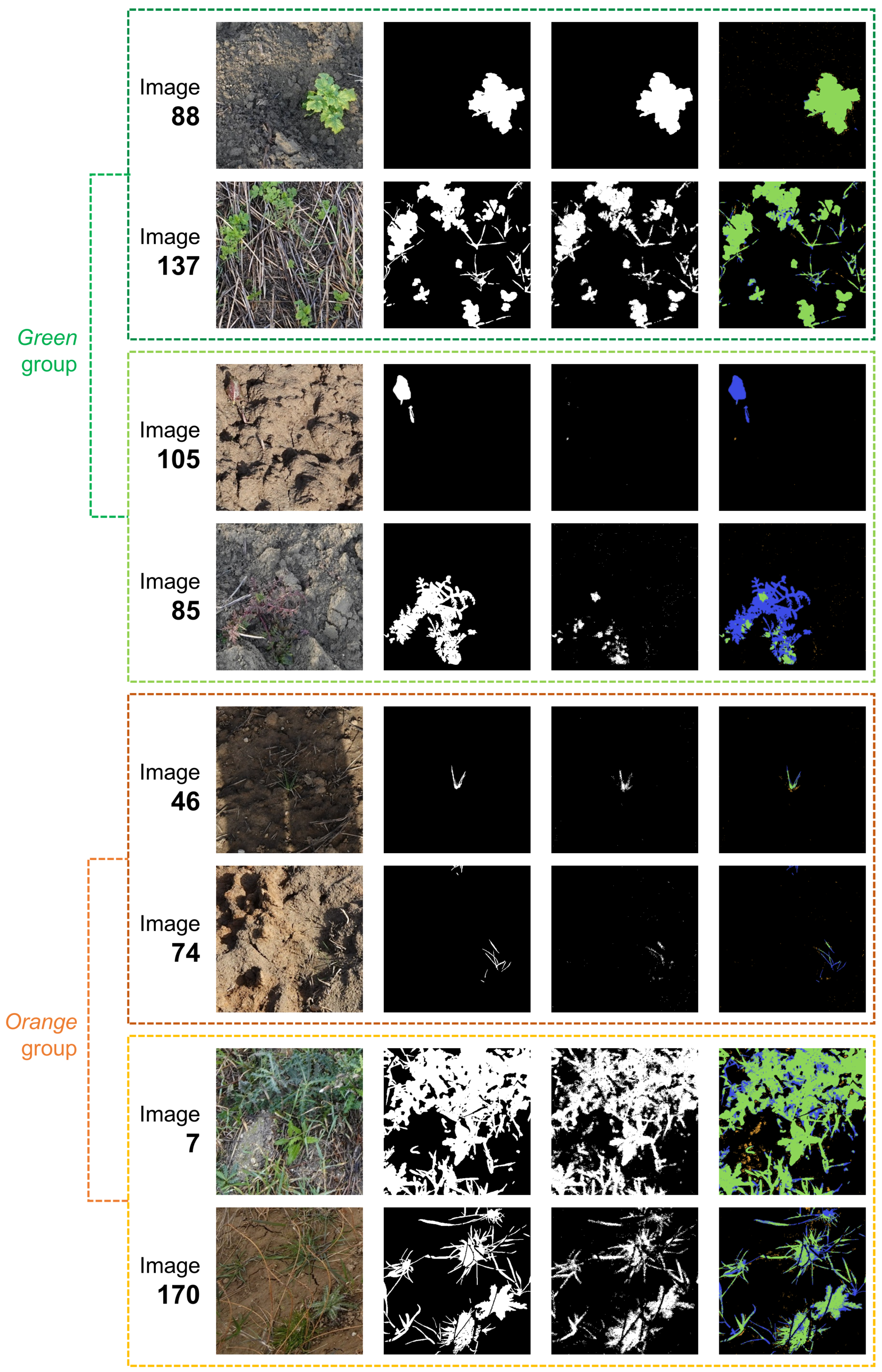
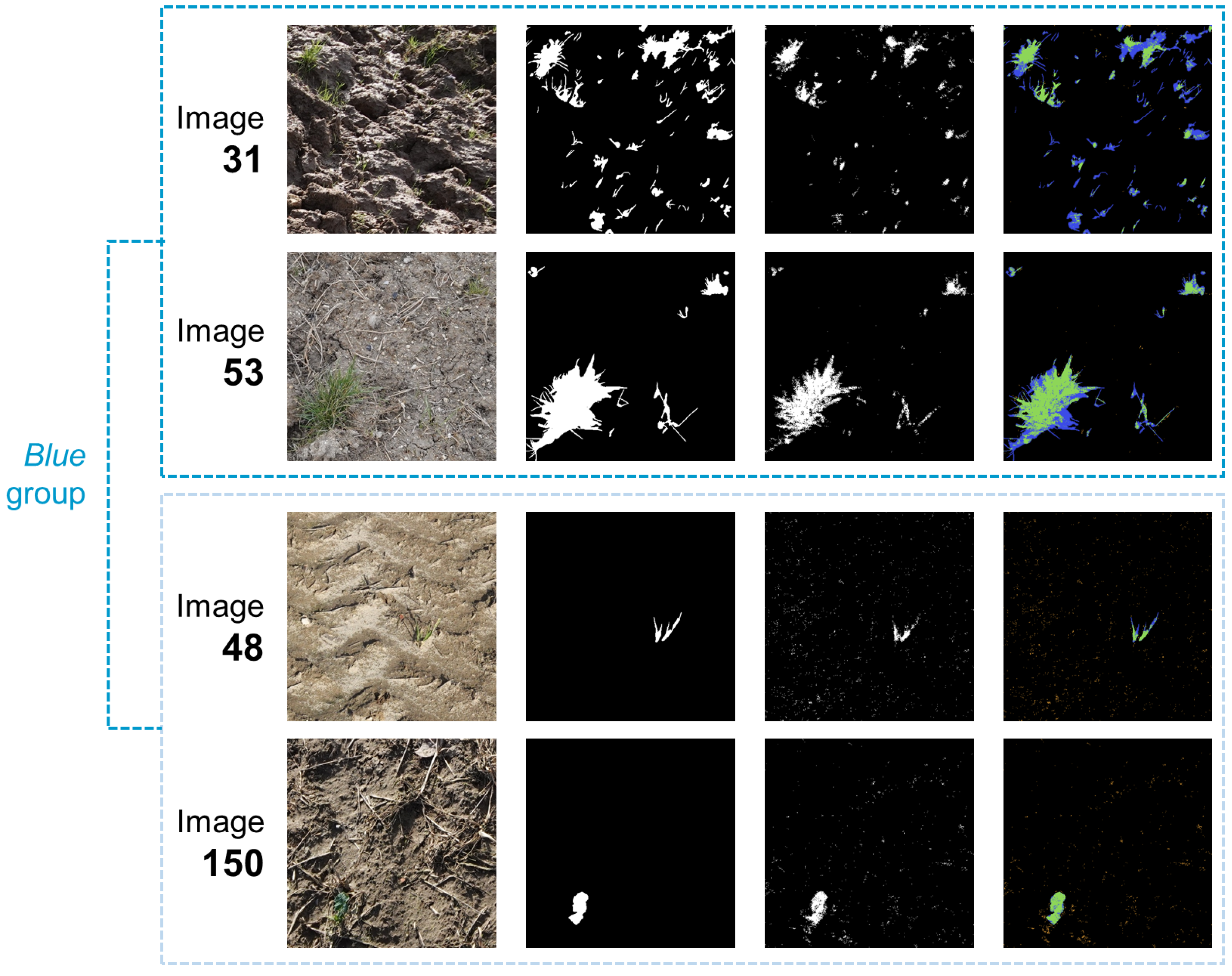
3.2. Visual Inspection of the Segmentation Masks
3.3. Multiple Factor Analysis
4. Conclusions
Author Contributions
Funding
Institutional Review Board Statement
Informed Consent Statement
Data Availability Statement
Acknowledgments
Conflicts of Interest
Abbreviations
| ACC | Accuracy |
| AMI | Adjusted Mutual Information |
| BAC | Balanced Accuracy |
| CIVE | Colour Index of Vegetation Extraction |
| DTSM | Decision Tree Segmentation Model |
| F1S | F1-Score |
| GCE | Global Consistency Error |
| HDD | Hausdorff Distance |
| IOU | Intersection Over Union |
| KAP | Cohen’s Kappa |
| MFA | Multiple Factor Analysis |
| NPV | Negative Predictive Value |
| PCA | Principal Component Analysis |
| PRC | Precision |
| RCL | Recall |
| RVA | Relative Vegetation Area |
| SVM | Support Vector Machine |
References
- Salzberg, S.L. On Comparing Classifiers: A Critique of Current Research and Methods. In Data Mining and Knowledge Discovery; Kluwer Academic Publishers: Boston, MA, USA, 1999. [Google Scholar]
- Zheng, A. Evaluating Machine Learning Models; O’Reilly Media, Inc.: Sepastopol, CA, USA, 2015. [Google Scholar]
- Sokolova, M.; Japkowicz, N.; Szpakowicz, S. Beyond Accuracy, F-Score and ROC: A Family of Discriminant Measures for Performance Evaluation. In AI 2006: Advances in Artificial Intelligence; Sattar, A., Kang, B.H., Eds.; Springer: Berlin/Heidelberg, Germany, 2006; Volume 4304, pp. 1015–1021. [Google Scholar] [CrossRef] [Green Version]
- Brodersen, K.H.; Ong, C.S.; Stephan, K.E.; Buhmann, J.M. The Balanced Accuracy and Its Posterior Distribution. In Proceedings of the 2010 20th International Conference on Pattern Recognition, Istanbul, Turkey, 23–26 August 2010; IEEE: Istanbul, Turkey, 2010; pp. 3121–3124. [Google Scholar] [CrossRef]
- D’Amour, A.; Heller, K.; Moldovan, D.; Adlam, B.; Alipanahi, B.; Beutel, A.; Chen, C.; Deaton, J.; Eisenstein, J.; Hoffman, M.D.; et al. Underspecification Presents Challenges for Credibility in Modern Machine Learning. arXiv 2020, arXiv:2011.03395. [Google Scholar]
- Gudivada, V.; Apon, A.; Ding, J. Data Quality Considerations for Big Data and Machine Learning: Going Beyond Data Cleaning and Transformations. Int. J. Adv. Softw. 2017, 10, 1–20. [Google Scholar]
- Breck, E.; Zinkevich, M.; Polyzotis, N.; Whang, S.; Roy, S. Data Validation for Machine Learning. In Proceedings of the SysML, Palo Alto, CA, USA, 31 March–2 April 2019. [Google Scholar]
- Jain, A.; Patel, H.; Nagalapatti, L.; Gupta, N.; Mehta, S.; Guttula, S.; Mujumdar, S.; Afzal, S.; Sharma Mittal, R.; Munigala, V. Overview and Importance of Data Quality for Machine Learning Tasks. In Proceedings of the 26th ACM SIGKDD International Conference on Knowledge Discovery & Data Mining, Virtual. 6–10 July 2020; Association for Computing Machinery: New York, NY, USA, 2020. KDD ’20. pp. 3561–3562. [Google Scholar] [CrossRef]
- Voulodimos, A.; Doulamis, N.; Doulamis, A.; Protopapadakis, E. Deep learning for computer vision: A brief review. Comput. Intell. Neurosci. 2018, 2018, 7068349. [Google Scholar] [CrossRef] [PubMed]
- Ponti, M.A.; Ribeiro, L.S.F.; Nazare, T.S.; Bui, T.; Collomosse, J. Everything You Wanted to Know about Deep Learning for Computer Vision but Were Afraid to Ask. In Proceedings of the 2017 30th SIBGRAPI Conference on Graphics, Patterns and Images Tutorials (SIBGRAPI-T), Rio de Janeiro, Brazil, 17–20 October 2017; pp. 17–41. [Google Scholar] [CrossRef] [Green Version]
- Ouhami, M.; Hafiane, A.; Es-Saady, Y.; El Hajji, M.; Canals, R. Computer Vision, IoT and Data Fusion for Crop Disease Detection Using Machine Learning: A Survey and Ongoing Research. Remote Sens. 2021, 13, 2486. [Google Scholar] [CrossRef]
- Caruana, R.; Niculescu-Mizil, A. Data mining in metric space: An empirical analysis of supervised learning performance criteria. In Proceedings of the 2004 ACM SIGKDD International Conference on Knowledge Discovery and Data Mining—KDD’04, Seattle, WA, USA, 22–25 August 2004; ACM Press: Seattle, WA, USA, 2004; p. 69. [Google Scholar] [CrossRef]
- Alaiz-Rodriguez, R.; Japkowicz, N.; Tischer, P. Visualizing Classifier Performance on Different Domains. In Proceedings of the 2008 20th IEEE International Conference on Tools with Artificial Intelligence, Dayton, OH, USA, 3–5 November 2008; Volume 2, pp. 3–10. [Google Scholar] [CrossRef] [Green Version]
- Seliya, N.; Khoshgoftaar, T.M.; Van Hulse, J. A Study on the Relationships of Classifier Performance Metrics. In Proceedings of the 2009 21st IEEE International Conference on Tools with Artificial Intelligence, Newark, NJ, USA, 2–4 November 2009; IEEE: Newark, NJ, USA, 2009; pp. 59–66. [Google Scholar] [CrossRef]
- Rakhmatuiln, I.; Kamilaris, A.; Andreasen, C. Deep Neural Networks to Detect Weeds from Crops in Agricultural Environments in Real-Time: A Review. Remote Sens. 2021, 13, 4486. [Google Scholar] [CrossRef]
- Sharma, A.; Jain, A.; Gupta, P.; Chowdary, V. Machine Learning Applications for Precision Agriculture: A Comprehensive Review. IEEE Access 2021, 9, 4843–4873. [Google Scholar] [CrossRef]
- Mavridou, E.; Vrochidou, E.; Papakostas, G.A.; Pachidis, T.; Kaburlasos, V.G. Machine Vision Systems in Precision Agriculture for Crop Farming. J. Imaging 2019, 5, 89. [Google Scholar] [CrossRef] [PubMed] [Green Version]
- Barrow, H.G.; Tenenbaum, J.M. Recovering Intrinsic Scene Characteristics from Images. In Computer Vision Systems; Academic Press: Waltham, MA, USA, 1978. [Google Scholar]
- Fieguth, P. Statistical Image Processing and Multidimensional Modeling; Information Science and Statistics; Springer: New York, NY, USA, 2011. [Google Scholar]
- Taha, A.A.; Hanbury, A. Metrics for evaluating 3D medical image segmentation: Analysis, selection, and tool. BMC Med. Imaging 2015, 15, 29. [Google Scholar] [CrossRef] [PubMed] [Green Version]
- Mittal, H.; Pandey, A.C.; Saraswat, M.; Kumar, S.; Pal, R.; Modwel, G. A comprehensive survey of image segmentation: Clustering methods, performance parameters, and benchmark datasets. Multimed. Tools Appl. 2021. [Google Scholar] [CrossRef] [PubMed]
- Li, Y.; Huang, Z.; Cao, Z.; Lu, H.; Wang, H.; Zhang, S. Performance Evaluation of Crop Segmentation Algorithms. IEEE Access 2020, 8, 36210–36225. [Google Scholar] [CrossRef]
- Guo, W.; Rage, U.K.; Ninomiya, S. Illumination invariant segmentation of vegetation for time series wheat images based on decision tree model. Comput. Electron. Agric. 2013, 96, 58–66. [Google Scholar] [CrossRef]
- Kohavi, R.; John, G.H. Wrappers for feature subset selection. Artif. Intell. 1997, 97, 273–324. [Google Scholar] [CrossRef] [Green Version]
- Breiman, L. (Ed.) Classification and Regression Trees, 1st ed.; Chapman & Hall/CRC: Boca Raton, FL, USA, 1998. [Google Scholar]
- Rico-Fernández, M.; Rios-Cabrera, R.; Castelán, M.; Guerrero-Reyes, H.I.; Juarez-Maldonado, A. A contextualized approach for segmentation of foliage in different crop species. Comput. Electron. Agric. 2019, 156, 378–386. [Google Scholar] [CrossRef]
- Vapnik, V.N. The Nature of Statistical Learning Theory, 2nd ed.; Statistics for Engineering and Information Science; Springer: Berlin, Germany, 2010. [Google Scholar]
- Kataoka, T.; Kaneko, T.; Okamoto, H.; Hata, S. Crop growth estimation system using machine vision. In Proceedings of the 2003 IEEE/ASME International Conference on Advanced Intelligent Mechatronics (AIM 2003), Kobe, Japan, 20–24 July 2003; Volume 2, pp. b1079–b1083. [Google Scholar] [CrossRef]
- Rijsbergen, C.J.V. Information Retrieval, 2nd ed.; Butterworth-Heinemann: Newton, MA, USA, 1979. [Google Scholar]
- Martin, D.; Fowlkes, C.; Tal, D.; Malik, J. A database of human segmented natural images and its application to evaluating segmentation algorithms and measuring ecological statistics. In Proceedings of the Eighth IEEE International Conference on Computer Vision, ICCV 2001, Vancouver, BC, Canada, 7–14 July 2001; IEEE Computer Society: Vancouver, BC, Canada, 2001; Volume 2, pp. 416–423. [Google Scholar] [CrossRef] [Green Version]
- Suh, H.K.; Hofstee, J.W.; van Henten, E.J. Improved vegetation segmentation with ground shadow removal using an HDR camera. Precis. Agric. 2018, 19, 218–237. [Google Scholar] [CrossRef] [Green Version]
- Pedregosa, F.; Varoquaux, G.; Gramfort, A.; Michel, V.; Thirion, B.; Grisel, O.; Blondel, M.; Prettenhofer, P.; Weiss, R.; Dubourg, V.; et al. Scikit-learn: Machine Learning in Python. J. Mach. Learn. Res. 2011, 12, 2825–2830. [Google Scholar]
- Vinh, N.X.; Epps, J.; Bailey, J. Information Theoretic Measures for Clusterings Comparison: Is a Correction for Chance Necessary? In Proceedings of the 26th Annual International Conference on Machine Learning, Montreal, QC, Canada, 14–18 June 2009; Association for Computing Machinery: New York, NY, USA, 2009. ICML’09. pp. 1073–1080. [Google Scholar] [CrossRef]
- Hausdorff, F. Grundzüge der Mengenlehre; Goschens Lehrbücherei/Gruppe I: Reine und Angewandte Mathematik Series; Von Veit; Verlag von Veit & Comp.: Leipzig, Germany, 1914. [Google Scholar]
- Huttenlocher, D.; Klanderman, G.; Rucklidge, W. Comparing images using the Hausdorff distance. IEEE Trans. Pattern Anal. Mach. Intell. 1993, 15, 850–863. [Google Scholar] [CrossRef] [Green Version]
- De la Torre, F.; Black, M. Robust principal component analysis for computer vision. In Proceedings of the Eighth IEEE International Conference on Computer Vision, ICCV 2001, Vancouver, BC, Canada, 7–14 July 2001; Volume 1, pp. 362–369. [Google Scholar] [CrossRef]
- Heumann, C.; Schomaker, M.; Shalabh. Introduction to Statistics and Data Analysis: With Exercises, Solutions and Applications in R, 2016 ed.; Springer International Publishing: Berlin, Germany, 2016. [Google Scholar]
- Chavent, M.; Kuentz-Simonet, V.; Liquet, B.; Saracco, J. ClustOfVar: An R Package for the Clustering of Variables. J. Stat. Softw. 2012, 50, 1–16. [Google Scholar] [CrossRef] [Green Version]
- Joliffe, I. Principal Component Analysis; Springer Series in Statistics; Springer: Berlin, Germany, 2002. [Google Scholar] [CrossRef]
- Abdi, H.; Williams, L.J. Principal component analysis. WIREs Comput. Stat. 2010, 2, 433–459. [Google Scholar] [CrossRef]
- Lê, S.; Josse, J.; Husson, F. FactoMineR: An R Package for Multivariate Analysis. J. Stat. Softw. 2008, 25, 1–18. [Google Scholar] [CrossRef] [Green Version]
- Escofier, B.; Pagès, J. Analyses Factorielles Simples et Multiples: Objectifs, Méthodes et Interpétation; Dunod: Paris, France, 2008. [Google Scholar]
- Abdi, H.; Williams, L.J.; Valentin, D. Multiple factor analysis: Principal component analysis for multitable and multiblock datasets: Multiple factor analysis. WIREs Comput. Stat. 2013, 5, 149–179. [Google Scholar] [CrossRef]
- Husson, F.; Josse, J.; Pagès, J. Principal Component Methods—Hierarchical Clustering—Partitional Clustering: Why Would We Need to Choose for Visualizing Data? Technical Report; Agrocampus Ouest: Rennes, France, 2021. [Google Scholar]


Publisher’s Note: MDPI stays neutral with regard to jurisdictional claims in published maps and institutional affiliations. |
© 2022 by the authors. Licensee MDPI, Basel, Switzerland. This article is an open access article distributed under the terms and conditions of the Creative Commons Attribution (CC BY) license (https://creativecommons.org/licenses/by/4.0/).
Share and Cite
Melki, P.; Bombrun, L.; Millet, E.; Diallo, B.; ElChaoui ElGhor, H.; Da Costa, J.-P. Exploratory Analysis on Pixelwise Image Segmentation Metrics with an Application in Proximal Sensing. Remote Sens. 2022, 14, 996. https://doi.org/10.3390/rs14040996
Melki P, Bombrun L, Millet E, Diallo B, ElChaoui ElGhor H, Da Costa J-P. Exploratory Analysis on Pixelwise Image Segmentation Metrics with an Application in Proximal Sensing. Remote Sensing. 2022; 14(4):996. https://doi.org/10.3390/rs14040996
Chicago/Turabian StyleMelki, Paul, Lionel Bombrun, Estelle Millet, Boubacar Diallo, Hakim ElChaoui ElGhor, and Jean-Pierre Da Costa. 2022. "Exploratory Analysis on Pixelwise Image Segmentation Metrics with an Application in Proximal Sensing" Remote Sensing 14, no. 4: 996. https://doi.org/10.3390/rs14040996
APA StyleMelki, P., Bombrun, L., Millet, E., Diallo, B., ElChaoui ElGhor, H., & Da Costa, J.-P. (2022). Exploratory Analysis on Pixelwise Image Segmentation Metrics with an Application in Proximal Sensing. Remote Sensing, 14(4), 996. https://doi.org/10.3390/rs14040996