
Geographical Detection of Urban Thermal Environment Based on the Local Climate Zones: A Case Study in Wuhan, China


Abstract
:1. Introduction
2. Research Methods
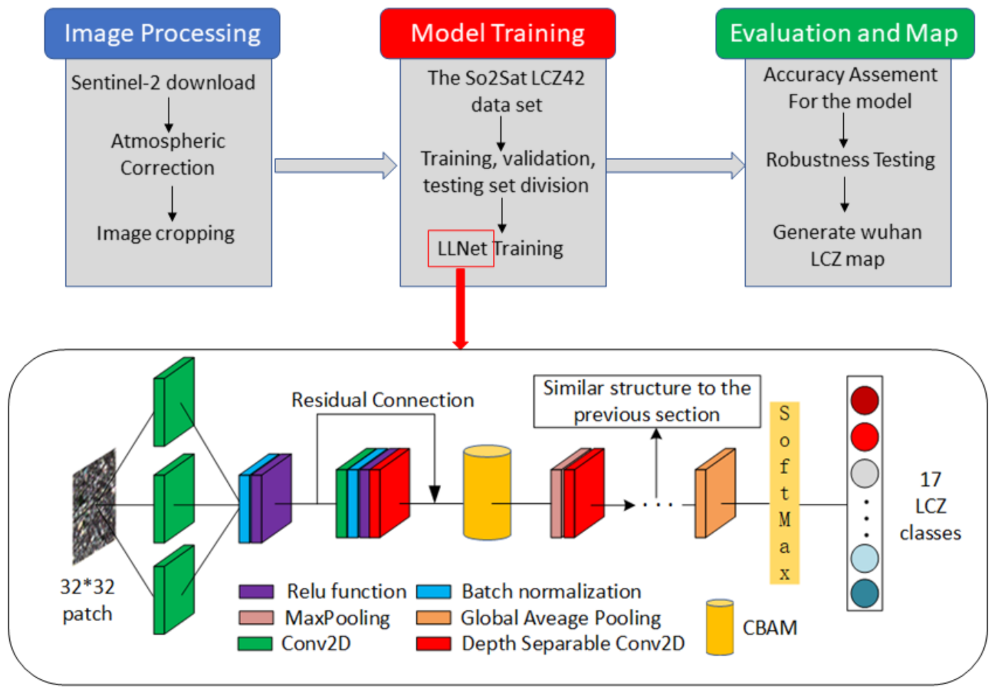
2.1. Remote Sensing Image Classification Based on Deep Learning
2.2. Geodetector Model
3. Study Area and Data
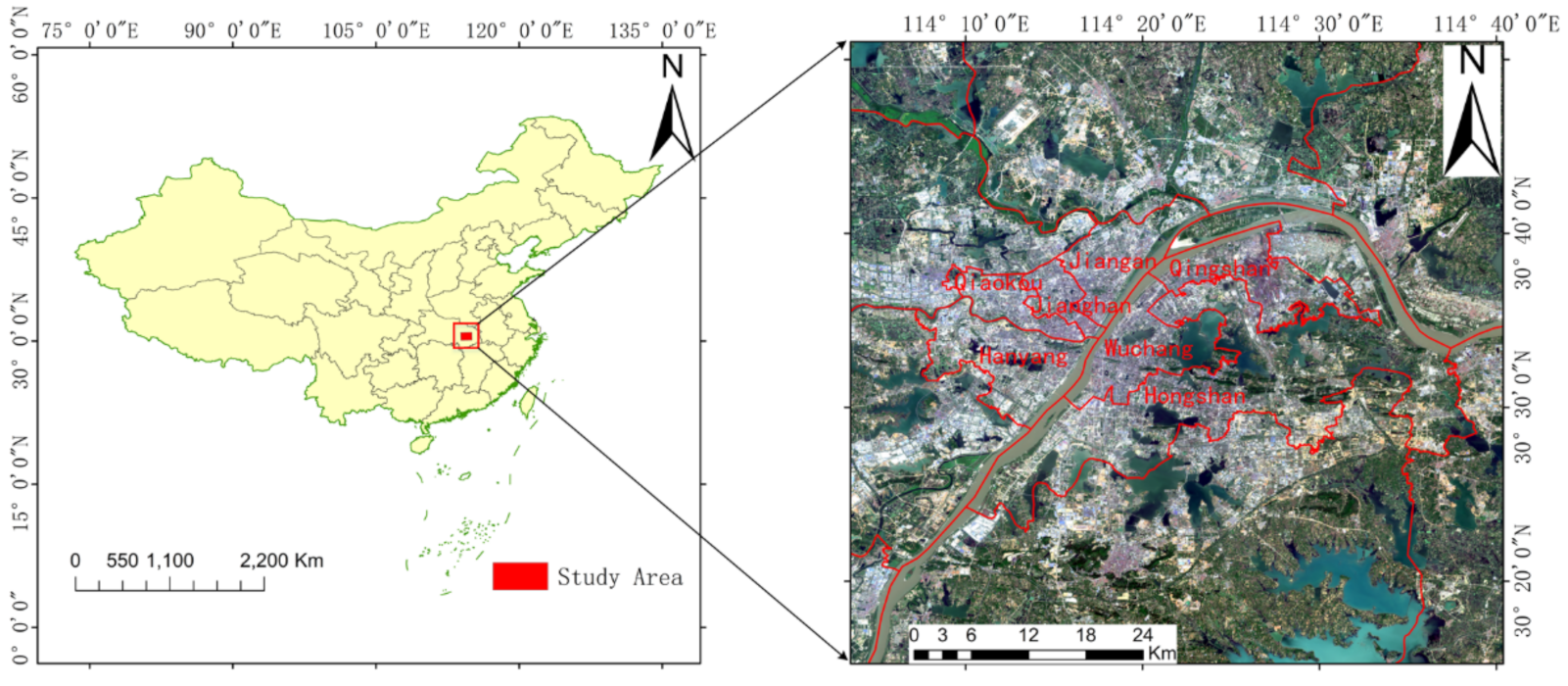
3.1. Study Area
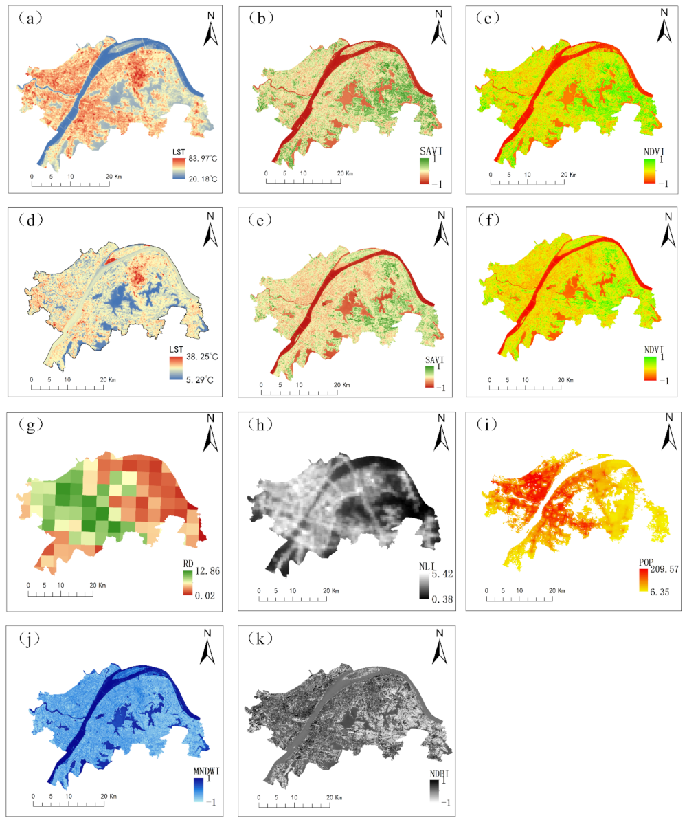
3.2. Multisource Driving Factor Data
4. Results
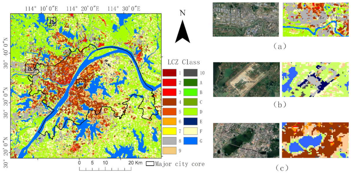
4.1. Mapping of LCZs
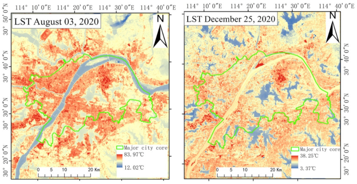
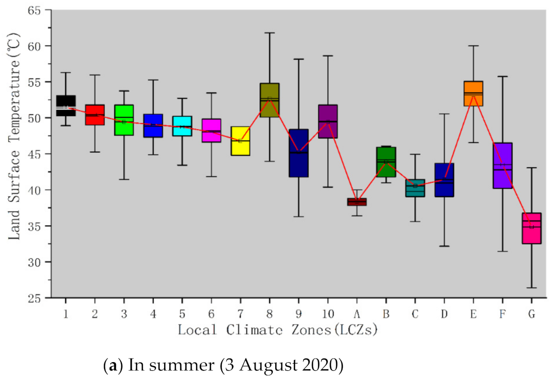
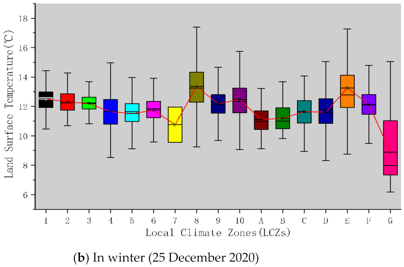
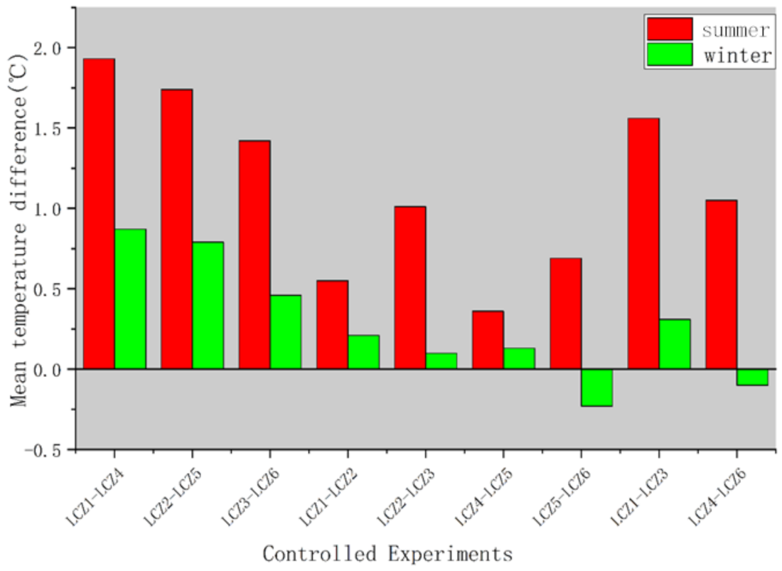
4.2. Study on Wuhan Urban Thermal Environment Based on LCZs
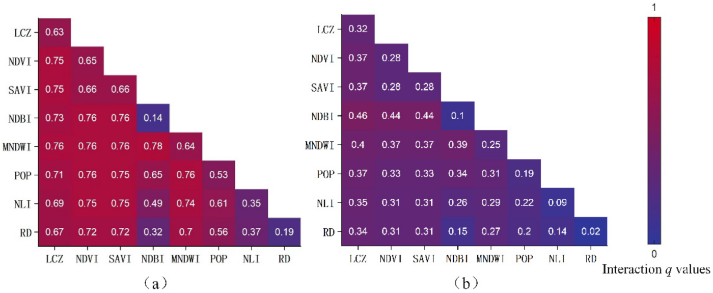
4.3. Spatial Differentiation Driving Interaction Mechanism of LST in Wuhan
5. Discussion
5.1. Accuracy of LCZ Classification
5.2. Uncertainties in Geographical Detection
5.3. Implications for Urban Environment Management
6. Conclusions
Author Contributions
Funding
Data Availability Statement
Acknowledgments
Conflicts of Interest
Appendix A

| Built Types | Definition | Land Cover Types | Definition |
|---|---|---|---|
 | Dense mix of tall buildings to tens of stories. Few or no trees. Land cover mostly paved. Concrete, steel, stone, and glass construction materials. |
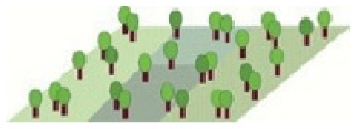
 | Landscape of wooded deciduous and evergreen trees. The land cover is mainly permeable. Representative areas include natural forests. |
 | Dense mix of midrise buildings (3–9 stories). Few or no trees. Land cover mostly paved. Stone, brick, tile, and concrete construction materials. |
 | Lightly wooded landscape of deciduous and/or evergreen trees. Land cover mostly pervious (low plants). Representative areas include urban park. |
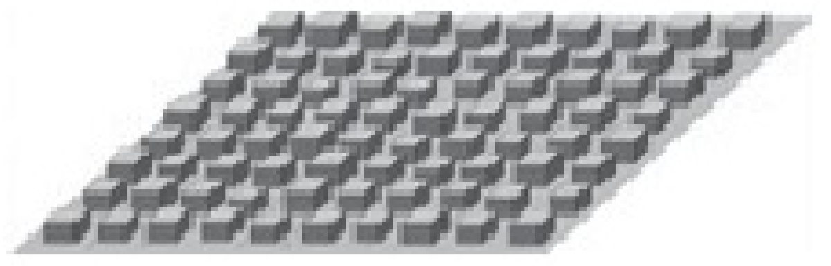 | Dense mix of low-rise buildings (1–3 stories). Few or no trees. Land cover mostly paved. Stone, brick, tile, and concrete construction materials. |
 | Open arrangement of bushes, shrubs, and short, woody trees. Land cover mostly pervious (bare soil or sand). |
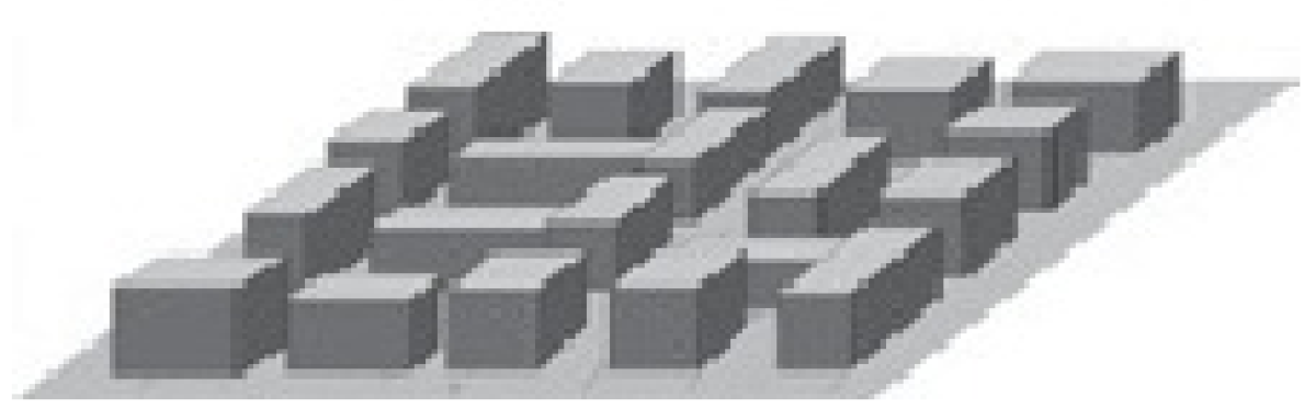
 | Open arrangement of tall buildings to tens of stories. Abundance of pervious land cover. Concrete, steel, and glass construction materials. |
 | Featureless landscape of grass or herbaceous plants/crops. Few or no trees. Zone function is natural grassland, agriculture or urban park. |
 | Open arrangement of midrise buildings (3–9 stories). Abundance of pervious land cover (low plants, scattered trees). |
 | Featureless landscape of rock or paved cover. Few or no trees or plants. Zone function is natural desert (rock) or urban transportation. |
 | Open arrangement of low-rise buildings (1–3 stories). Abundance of pervious land cover (low plants, scattered trees). |
 | Featureless landscape of soil or sand cover. Few or no trees or plants. Zone function is natural desert or agriculture. |
 | Dense mix of single-story buildings. Few or no trees. Land cover mostly hard-packed. Lightweight construction materials. |
 | Large, open water bodies, such as seas and lakes, or small bodies, such as rivers, reservoirs, and lagoons. |
 | Open arrangement of large low-rise buildings (1–3 stories). Few or no trees. Land cover mostly paved. Steel and stone construction materials. | Additional Land Cover Classes
| |
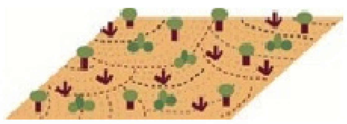
 | Sparse arrangement of small or medium-sized buildings in a natural setting. Abundance of pervious land cover (low plants, scattered trees). | ||
 | Low-rise and mid-rise industrial structures (towers, tanks, stacks). Few or no trees. Land cover mostly paved or hard-packed. | ||
Appendix B
| Research Question | Study Area | Dependent Variable Y | Independent Variable X | Literature |
|---|---|---|---|---|
| Factors influencing hand, foot and mouth disease | China | Hand, foot and mouth disease incidence | Monthly average temperature, monthly precipitation, relative humidity, population density, primary school density, secondary school density, GDP, industrial structure | [76] |
| Controlling factors of urban landscape | Fujian Xiamen China | Connectivity of forest landscape | Weather, FMPl, elevation, population | [37] |
| Potential driving factors of landsurface temperature | Tianjin, China | Landsurface temperature | NDVI, TCG, SAVl, NDBI, MNDWI, TCW, WD, NLI, RD, RWD | [71] |
| Influence of human activities and ecological factors on urban surface temperature | Xiamen, China | Urban forest temperature | Population density, woodland survey, DEM, remote sensing image, etc | [77] |
| Factor analysis of industral CO2 emissions | Inner Mongolia, China | CO2 emissions | GDP, industrial structure, urbanization rate, economic growth rate population and road density | [78] |
| Identification of influe ncing factors of continental surface cutting degree | The United States | Degree of epicontinental cutting | Climate, slope, topography, rock, soil, vegetation | [79] |
Appendix C
| LCZ | Sky View Factor | Aspect Ratio | Building Surface Fraction | Impervious Surface Fraction | Pervious Surface Fraction | Height of Roughness Elements | Terrain Roughness Class | Surface Admittance | Surface Albedo | Anthropogenic Heat Output |
|---|---|---|---|---|---|---|---|---|---|---|
| LCZ 1 Compact high-rise | 0.2–0.4 | >2 | 40–60 | 40–60 | <10 | >25 | 8 | 1500–1800 | 0.10–0.20 | 50–300 |
| LCZ 2 Compact midrise | 0.3–0.6 | 0.75–2 | 40–70 | 30–50 | <20 | 10–25 | 6–7 | 1500–2200 | 0.10–0.20 | <75 |
| LCZ 3 Compact low-rise | 0.2–0.6 | 0.75–1.5 | 40–70 | 20–50 | <30 | 3–10 | 6 | 1200–1800 | 0.10–0.20 | <75 |
| LCZ 4 Open high-rise | 0.5–0.7 | 0.75–1.25 | 20–40 | 30–40 | 30–40 | >25 | 7–8 | 1400–1800 | 0.12–0.25 | <50 |
| LCZ 5 Open midrise | 0.5–0.8 | 0.3–0.75 | 20–40 | 30–50 | 20–40 | 10–25 | 5–6 | 1400–2000 | 0.12–0.25 | <25 |
| LCZ 6 Open low-rise | 0.6–0.9 | 0.3–0.75 | 20–40 | 20–50 | 30–60 | 3–10 | 5–6 | 1200–1800 | 0.12–0.25 | <25 |
| LCZ 7 Lightweight low-rise | 0.2–0.5 | 1–2 | 60–90 | <20 | <30 | 2–4 | 4–5 | 800–1500 | 0.15–0.35 | <35 |
| LCZ 8 Large low-rise | >0.7 | 0.1–0.3 | 30–50 | 40–50 | <20 | 3–10 | 5 | 1200–1800 | 0.15–0.25 | <50 |
| LCZ 9 Sparsely built | >0.8 | 0.1–0.25 | 10–20 | <20 | 60–80 | 3–10 | 5–6 | 1000–1800 | 0.12–0.25 | <10 |
| LCZ 10 Heavy industry | 0.6–0.9 | 0.2–0.5 | 20–30 | 20–40 | 40–50 | 5–15 | 5–6 | 1000–2500 | 0.12–0.20 | >300 |
| LCZ A Dense trees | <0.4 | >1 | <10 | <10 | >90 | 3–30 | 8 | unknown | 0.10–0.20 | 0 |
| LCZ B Scattered trees | 0.5–0.8 | 0.25–0.75 | <10 | <10 | >90 | 3–15 | 5–6 | 1000–1800 | 0.15–0.25 | 0 |
| LCZ C Bush, scrub | 0.7–0.9 | 0.25–1.0 | <10 | <10 | >90 | <2 | 4–5 | 700–1500 | 0.15–0.30 | 0 |
| LCZ D Low plants | >0.9 | <0.1 | <10 | <10 | >90 | <1 | 3–4 | 1200–1600 | 0.15–0.25 | 0 |
| LCZ E Bare rock or paved | >0.9 | <0.1 | <10 | >90 | <10 | <0.25 | 1–2 | 1200–2500 | 0.15–0.30 | 0 |
| LCZ F Bare soil or sand | >0.9 | <0.1 | <10 | <10 | >90 | <0.25 | 1–2 | 600–1400 | 0.20–0.35 | 0 |
| LCZ G Water | >0.9 | <0.1 | <10 | <10 | >90 | – | 1 | 1500 | 0.02–0.10 | 0 |
References
- Cohen, B. Urbanization, City growth, and the New United Nations development agenda. Cornerstone 2015, 3, 4–7. [Google Scholar]
- Liu, Z.; He, C.; Zhou, Y.; Wu, J. How much of the world’s land has been urbanized, really? A hierarchical framework for avoiding confusion. Landsc. Ecol. 2014, 29, 763–771. [Google Scholar] [CrossRef]
- Yusuf, Y.A.; Pradhan, B.; Idrees, M.O. Spatio-temporal assessment of urban heat island effects in Kuala Lumpur metropolitan city using landsat images. J. Indian Soc. Remote Sens. 2014, 42, 829–837. [Google Scholar] [CrossRef]
- Wang, Y.; Du, H.; Xu, Y.; Lu, D.; Wang, X.; Guo, Z. Temporal and spatial variation relationship and influence factors on surface urban heat island and ozone pollution in the Yangtze River Delta, China. Sci. Total Environ. 2018, 631, 921–933. [Google Scholar] [CrossRef] [PubMed]
- Arnfield, A.J. Two decades of urban climate research: A review of turbulence, exchanges of energy and water, and the urban heat island. Int. J. Climatol. J. R. Meteorol. Soc. 2003, 23, 1–26. [Google Scholar] [CrossRef]
- Kalisa, E.; Fadlallah, S.; Amani, M.; Nahayo, L.; Habiyaremye, G. Temperature and air pollution relationship during heatwaves in Birmingham, UK. Sustain. Cities Soc. 2018, 43, 111–120. [Google Scholar] [CrossRef] [Green Version]
- Mayrhuber, E.A.-S.; Dückers, M.L.; Wallner, P.; Arnberger, A.; Allex, B.; Wiesböck, L.; Wanka, A.; Kolland, F.; Eder, R.; Hutter, H.-P. Vulnerability to heatwaves and implications for public health interventions—A scoping review. Environ. Res. 2018, 166, 42–54. [Google Scholar] [CrossRef] [Green Version]
- Guo, Y.; Gasparrini, A.; Li, S.; Sera, F.; Vicedo-Cabrera, A.M.; de Sousa Zanotti Stagliorio Coelho, M.; Saldiva, P.H.N.; Lavigne, E.; Tawatsupa, B.; Punnasiri, K. Quantifying excess deaths related to heatwaves under climate change scenarios: A multicountry time series modelling study. PLoS Med. 2018, 15, e1002629. [Google Scholar] [CrossRef]
- Debbage, N.; Shepherd, J.M. The urban heat island effect and city contiguity. Comput. Environ. Urban. Syst. 2015, 54, 181–194. [Google Scholar] [CrossRef]
- Oke, T.R. City size and the urban heat island. Atmos. Environ. 1973, 7, 769–779. [Google Scholar] [CrossRef]
- Santamouris, M.; Cartalis, C.; Synnefa, A.; Kolokotsa, D. On the impact of urban heat island and global warming on the power demand and electricity consumption of buildings—A review. Energy Build. 2015, 98, 119–124. [Google Scholar] [CrossRef]
- Stewart, I.D.; Oke, T.R. Local climate zones for urban temperature studies. Bull. Am. Meteorol. Soc. 2012, 93, 1879–1900. [Google Scholar] [CrossRef]
- Stewart, I.D.; Oke, T.R.; Krayenhoff, E.S. Evaluation of the ‘local climate zone’scheme using temperature observations and model simulations. Int. J. Climatol. 2014, 34, 1062–1080. [Google Scholar] [CrossRef]
- Kaloustian, N.; Bechtel, B. Local climatic zoning and urban heat island in Beirut. Procedia Eng. 2016, 169, 216–223. [Google Scholar] [CrossRef]
- Cai, M.; Ren, C.; Xu, Y.; Lau, K.K.-L.; Wang, R. Investigating the relationship between local climate zone and land surface temperature using an improved WUDAPT methodology–A case study of Yangtze River Delta, China. Urban. Clim. 2018, 24, 485–502. [Google Scholar] [CrossRef]
- Bechtel, B.; Alexander, P.J.; Böhner, J.; Ching, J.; Conrad, O.; Feddema, J.; Mills, G.; See, L.; Stewart, I. Mapping local climate zones for a worldwide database of the form and function of cities. ISPRS Int. J. Geo-Inf. 2015, 4, 199–219. [Google Scholar] [CrossRef] [Green Version]
- Bechtel, B.; Alexander, P.J.; Beck, C.; Böhner, J.; Brousse, O.; Ching, J.; Demuzere, M.; Fonte, C.; Gál, T.; Hidalgo, J. Generating WUDAPT Level 0 data–Current status of production and evaluation. Urban. Clim. 2019, 27, 24–45. [Google Scholar] [CrossRef] [Green Version]
- Ching, J.; Mills, G.; Bechtel, B.; See, L.; Feddema, J.; Wang, X.; Ren, C.; Brousse, O.; Martilli, A.; Neophytou, M. WUDAPT: An urban weather, climate, and environmental modeling infrastructure for the anthropocene. Bull. Am. Meteorol. Soc. 2018, 99, 1907–1924. [Google Scholar] [CrossRef] [Green Version]
- Zhang, L.; Zhang, L.; Du, B. Deep learning for remote sensing data: A technical tutorial on the state of the art. IEEE Geosci. Remote Sens. Mag. 2016, 4, 22–40. [Google Scholar] [CrossRef]
- Liu, S.; Shi, Q. Local climate zone mapping as remote sensing scene classification using deep learning: A case study of metropolitan China. ISPRS J. Photogramm. Remote Sens. 2020, 164, 229–242. [Google Scholar] [CrossRef]
- Qiu, C.; Tong, X.; Schmitt, M.; Bechtel, B.; Zhu, X.X. Multilevel feature fusion-based CNN for local climate zone classification from sentinel-2 images: Benchmark results on the So2Sat LCZ42 dataset. IEEE J. Sel. Top. Appl. Earth Obs. Remote Sens. 2020, 13, 2793–2806. [Google Scholar] [CrossRef]
- Yoo, C.; Lee, Y.; Cho, D.; Im, J.; Han, D. Improving local climate zone classification using incomplete building data and Sentinel 2 images based on convolutional neural networks. Remote Sens. 2020, 12, 3552. [Google Scholar] [CrossRef]
- Shih, W. The impact of urban development patterns on thermal distribution in Taipei. In Proceedings of the 2017 Joint Urban Remote Sensing Event (JURSE), Dubai, United Arab Emirates, 6–8 March 2017; pp. 1–5. [Google Scholar]
- Geletič, J.; Lehnert, M.; Dobrovolný, P. Land surface temperature differences within local climate zones, based on two central European cities. Remote Sens. 2016, 8, 788. [Google Scholar] [CrossRef] [Green Version]
- Koc, C.B.; Osmond, P.; Peters, A.; Irger, M. Understanding land surface temperature differences of local climate zones based on airborne remote sensing data. IEEE J. Sel. Top. Appl. Earth Obs. Remote Sens. 2018, 11, 2724–2730. [Google Scholar]
- Zhao, C.; Jensen, J.L.; Weng, Q.; Currit, N.; Weaver, R. Use of Local Climate Zones to investigate surface urban heat islands in Texas. GIScience Remote Sens. 2020, 57, 1083–1101. [Google Scholar] [CrossRef]
- Richard, Y.; Emery, J.; Dudek, J.; Pergaud, J.; Chateau-Smith, C.; Zito, S.; Rega, M.; Vairet, T.; Castel, T.; Thévenin, T. How relevant are local climate zones and urban climate zones for urban climate research? Dijon (France) as a case study. Urban. Clim. 2018, 26, 258–274. [Google Scholar] [CrossRef] [Green Version]
- Mushore, T.D.; Dube, T.; Manjowe, M.; Gumindoga, W.; Chemura, A.; Rousta, I.; Odindi, J.; Mutanga, O. Remotely sensed retrieval of Local Climate Zones and their linkages to land surface temperature in Harare metropolitan city, Zimbabwe. Urban. Clim. 2019, 27, 259–271. [Google Scholar] [CrossRef]
- Verdonck, M.-L.; Demuzere, M.; Hooyberghs, H.; Beck, C.; Cyrys, J.; Schneider, A.; Dewulf, R.; Van Coillie, F. The potential of local climate zones maps as a heat stress assessment tool, supported by simulated air temperature data. Landsc. Urban Plan. 2018, 178, 183–197. [Google Scholar] [CrossRef]
- Yang, X.; Yao, L.; Jin, T.; Peng, L.L.; Jiang, Z.; Hu, Z.; Ye, Y. Assessing the thermal behavior of different local climate zones in the Nanjing metropolis, China. Build. Environ. 2018, 137, 171–184. [Google Scholar] [CrossRef]
- Zhongli, L.; Hanqiu, X. A study of urban heat island intensity based on “local climate zones”: A case study in Fuzhou, China. In Proceedings of the 2016 4th International Workshop on Earth Observation and Remote Sensing Applications (EORSA), Guangzhou, China, 4–6 July 2016; pp. 250–254. [Google Scholar]
- Chen, A.; Yao, L.; Sun, R.; Chen, L. How many metrics are required to identify the effects of the landscape pattern on land surface temperature? Ecol. Indic. 2014, 45, 424–433. [Google Scholar] [CrossRef]
- Huang, X.; Wang, Y. Investigating the effects of 3D urban morphology on the surface urban heat island effect in urban functional zones by using high-resolution remote sensing data: A case study of Wuhan, Central China. ISPRS J. Photogramm. Remote Sens. 2019, 152, 119–131. [Google Scholar] [CrossRef]
- Peng, J.; Jia, J.; Liu, Y.; Li, H.; Wu, J. Seasonal contrast of the dominant factors for spatial distribution of land surface temperature in urban areas. Remote Sens. Environ. 2018, 215, 255–267. [Google Scholar] [CrossRef]
- Peng, W.; Zhang, D.; Luo, Y.; Tao, S.; Xu, X. Influence of natural factors on vegetation NDVI using geographical detection in Sichuan Province. Acta Geogr. Sin. 2019, 74, 1758. [Google Scholar]
- Wang, J.; Xu, C. Geodetector: Principle and prospective. Acta Geogr. Sin. 2017, 72, 116–134. [Google Scholar]
- Ren, Y.; Deng, L.; Zuo, S.; Luo, Y.; Shao, G.; Wei, X.; Hua, L.; Yang, Y. Geographical modeling of spatial interaction between human activity and forest connectivity in an urban landscape of southeast China. Landsc. Ecol. 2014, 29, 1741–1758. [Google Scholar] [CrossRef]
- Han, Z.; Zhiyuan, R. Remote sensing analysis of vegetation phenology characteristics in Shaanxi province based on Whittaker smoother method. J. Desert Res. 2015, 35, 901–906. [Google Scholar]
- Liao, Y.; Zhang, Y.; He, L.; Wang, J.; Liu, X.; Zhang, N.; Xu, B. Temporal and spatial analysis of neural tube defects and detection of geographical factors in Shanxi Province, China. PLoS ONE 2016, 11, e0150332. [Google Scholar] [CrossRef]
- Zhou, L.; Wu, J.; Jia, R.; Liang, N.; Zhang, F.; Ni, Y.; Liu, M. Investigation of temporal-spatial characteristics and underlying risk factors of PM2. 5 pollution in Beijing-Tianjin-Hebei Area. Res. Environ. Sci. 2016, 29, 483–493. [Google Scholar]
- Ding, Y.; Cai, J.; Ren, Z.; Yang, Z. Spatial disparities of economic growth rate of China’s National-level ETDZs and their determinants based on geographical detector analysis. Prog. Geogr. 2014, 5, 657–666. [Google Scholar]
- Shuoben, B.; Han, J.; Changchun, C.; Hongru, Y.; Xiang, S. Application of geographical detector in human-environment relationship study of prehistoric settlements. Prog. Geogr. 2015, 34, 118–127. [Google Scholar]
- Yokoya, N.; Ghamisi, P.; Xia, J.; Sukhanov, S.; Heremans, R.; Tankoyeu, I.; Bechtel, B.; Le Saux, B.; Moser, G.; Tuia, D. Open data for global multimodal land use classification: Outcome of the 2017 IEEE GRSS Data Fusion Contest. IEEE J. Sel. Top. Appl. Earth Obs. Remote Sens. 2018, 11, 1363–1377. [Google Scholar] [CrossRef] [Green Version]
- Zhu, X.X.; Hu, J.; Qiu, C.; Shi, Y.; Kang, J.; Mou, L.; Bagheri, H.; Häberle, M.; Hua, Y.; Huang, R. So2Sat LCZ42: A benchmark dataset for global local climate zones classification. IEEE Geosci. Remote Sens. Mag. 2020, 8, 76–89. [Google Scholar] [CrossRef] [Green Version]
- He, K.; Zhang, X.; Ren, S.; Sun, J. Deep residual learning for image recognition. In Proceedings of the IEEE conference on computer vision and pattern recognition, Las Vegas, NV, USA, 27–30 June 2016; pp. 770–778. [Google Scholar]
- Woo, S.; Park, J.; Lee, J.-Y.; Kweon, I.S. Cbam: Convolutional block attention module. In Proceedings of the European Conference on Computer Vision (ECCV), Munich, Germany, 8–14 September 2014; pp. 3–19. [Google Scholar]
- Howard, A.G.; Zhu, M.; Chen, B.; Kalenichenko, D.; Wang, W.; Weyand, T.; Andreetto, M.; Adam, H. Mobilenets: Efficient convolutional neural networks for mobile vision applications. arXiv 2017, arXiv:1704.04861. [Google Scholar]
- Tobler, W.R. A computer movie simulating urban growth in the Detroit region. Econ. Geogr. 1970, 46, 234–240. [Google Scholar] [CrossRef]
- Tucker, C.J.; Vanpraet, C.L.; Sharman, M.; Van Ittersum, G. Satellite remote sensing of total herbaceous biomass production in the Senegalese Sahel: 1980–1984. Remote Sens. Environ. 1985, 17, 233–249. [Google Scholar] [CrossRef]
- Zha, Y.; Gao, J.; Ni, S. Use of normalized difference built-up index in automatically mapping urban areas from TM imagery. Int. J. Remote Sens. 2003, 24, 583–594. [Google Scholar] [CrossRef]
- Xu, H. Modification of normalised difference water index (NDWI) to enhance open water features in remotely sensed imagery. Int. J. Remote Sens. 2006, 27, 3025–3033. [Google Scholar] [CrossRef]
- Xu, H. A new index for delineating built-up land features in satellite imagery. Int. J. Remote Sens. 2008, 29, 4269–4276. [Google Scholar] [CrossRef]
- Cook, M.; Schott, J.R.; Mandel, J.; Raqueno, N. Development of an operational calibration methodology for the Landsat thermal data archive and initial testing of the atmospheric compensation component of a Land Surface Temperature (LST) product from the archive. Remote Sens. 2014, 6, 11244–11266. [Google Scholar] [CrossRef] [Green Version]
- Yao, R.; Wang, L.; Huang, X.; Zhang, W.; Li, J.; Niu, Z. Interannual variations insurface urban heat island intensity and associated drivers in China. J. Environ. Manag. 2018, 222, 86–94. [Google Scholar] [CrossRef] [PubMed]
- Yu, B.; Tang, M.; Wu, Q.; Yang, C.; Deng, S.; Shi, K.; Peng, C.; Wu, J.; Chen, Z. Urban built-up area extraction from log-transformed NPP-VIIRS nighttime light composite data. IEEE Geosci. Remote Sens. Lett. 2018, 15, 1279–1283. [Google Scholar] [CrossRef]
- Sun, Y.; Gao, C.; Li, J.; Li, W.; Ma, R. Examining urban thermal environment dynamics and relations to biophysical composition and configuration and socio-economic factors: A case study of the Shanghai metropolitan region. Sustain. Cities Soc. 2018, 40, 284–295. [Google Scholar] [CrossRef]
- Lloyd, C.T.; Sorichetta, A.; Tatem, A.J. High resolution global gridded data for use in population studies. Sci. Data 2017, 4, 1–17. [Google Scholar] [CrossRef] [PubMed] [Green Version]
- Unger, J.; Lelovics, E.; Gál, T. Local Climate Zone mapping using GIS methods in Szeged. Hung. Geogr. Bull. 2014, 63, 29–41. [Google Scholar] [CrossRef] [Green Version]
- Tripathy, B.R.; Sajjad, H.; Elvidge, C.D.; Ting, Y.; Pandey, P.C.; Rani, M.; Kumar, P. Modeling of electric demand for sustainable energy and management in India using spatio-temporal DMSP-OLS night-time data. Environ. Manag. 2018, 61, 615–623. [Google Scholar] [CrossRef]
- He, S.; Zhang, Y.; Gu, Z.; Su, J. Local climate zone classification with different source data in Xi’an, China. Indoor Built Environ. 2019, 28, 1190–1199. [Google Scholar] [CrossRef]
- Quan, J. Enhanced geographic information system-based mapping of local climate zones in Beijing, China. Sci. China Technol. Sci. 2019, 62, 2243–2260. [Google Scholar] [CrossRef]
- Yang, J.; Jin, S.; Xiao, X.; Jin, C.; Xia, J.C.; Li, X.; Wang, S. Local climate zone ventilation and urban land surface temperatures: Towards a performance-based and wind-sensitive planning proposal in megacities. Sustain. Cities Soc. 2019, 47, 101487. [Google Scholar] [CrossRef]
- Estoque, R.C.; Murayama, Y.; Myint, S.W. Effects of landscape composition and pattern on land surface temperature: An urban heat island study in the megacities of Southeast Asia. Sci. Total Environ. 2017, 577, 349–359. [Google Scholar] [CrossRef]
- Wang, M.; Zhang, Z.; Hu, T.; Liu, X. A practical single-channel algorithm for land surface temperature retrieval: Application to Landsat series data. J. Geophys. Res. Atmos. 2019, 124, 299–316. [Google Scholar] [CrossRef]
- Wang, M.; Zhang, Z.; Hu, T.; Wang, G.; He, G.; Zhang, Z.; Li, H.; Wu, Z.; Liu, X. An Efficient Framework for Producing Landsat-Based Land Surface Temperature Data Using Google Earth Engine. IEEE J. Sel. Top. Appl. Earth Obs. Remote Sens. 2020, 13, 4689–4701. [Google Scholar] [CrossRef]
- Gao, F.; Li, S.; Tan, Z.; Wu, Z.; Zhang, X.; Huang, G.; Huang, Z. Understanding the modifiable areal unit problem in dockless bike sharing usage and exploring the interactive effects of built environment factors. Int. J. Geogr. Inf. Sci. 2021, 35, 1905–1925. [Google Scholar] [CrossRef]
- Alexander, P.J.; Mills, G. Local climate classification and Dublin’s urban heat island. Atmosphere 2014, 5, 755–774. [Google Scholar] [CrossRef] [Green Version]
- Leconte, F.; Bouyer, J.; Claverie, R.; Pétrissans, M. Using Local Climate Zone scheme for UHI assessment: Evaluation of the method using mobile measurements. Build. Environ. 2015, 83, 39–49. [Google Scholar] [CrossRef]
- Wang, Y.; Zhan, Q.; Ouyang, W. Impact of urban climate landscape patterns on land surface temperature in Wuhan, China. Sustainability 2017, 9, 1700. [Google Scholar] [CrossRef] [Green Version]
- Javanroodi, K.; Mahdavinejad, M.; Nik, V.M. Impacts of urban morphology on reducing cooling load and increasing ventilation potential in hot-arid climate. Appl. Energy 2018, 231, 714–746. [Google Scholar] [CrossRef]
- Hu, D.; Meng, Q.; Zhang, L.; Zhang, Y. Spatial quantitative analysis of the potential driving factors of land surface temperature in different “Centers” of polycentric cities: A case study in Tianjin, China. Sci. Total Environ. 2020, 706, 135244. [Google Scholar] [CrossRef]
- Chen, D.; Hu, M.; Guo, Y.; Dahlgren, R.A. Changes in river water temperature between 1980 and 2012 in Yongan watershed, eastern China: Magnitude, drivers and models. J. Hydrol. 2016, 533, 191–199. [Google Scholar] [CrossRef] [Green Version]
- Sinokrot, B.A.; Stefan, H.G. Stream temperature dynamics: Measurements and modeling. Water Resour. Res. 1993, 29, 2299–2312. [Google Scholar] [CrossRef]
- Li, J.; Xia, Z.; Wang, Y. Impact of the Three Gorges and Gezhouba reservoirs on ecohydrological conditions for sturgeon in the Yangtze River, China. J. Hydrol. Eng. 2013, 18, 1563–1570. [Google Scholar] [CrossRef]
- Hong, T.L.Y.; Lv, H.; Meng, B.; Bi, S.; Zhou, L. Patterns of Phytoplankton Phenology and Its Response to Temperature of Water Surface in Lake Taihu based on MODIS Data. J. Geo-Inf. Sci. 2020, 22, 1935–1945. [Google Scholar]
- Huang, J.; Wang, J.; Bo, Y.; Xu, C.; Hu, M.; Huang, D. Identification of health risks of hand, foot and mouth disease in China using thegeographical detector technique. Int. J. Environ. Res. Public Health 2014, 11, 3407–3423. [Google Scholar] [CrossRef]
- Ren, Y.; Deng, L.; Zuo, S.; Song, X.; Liao, Y.; Xu, C.; Chen, Q.; Hua, L.; Li, Z. Quantifying the influences of various ecological factors on land surface temperature of urban forests. Environ. Pollut. 2016, 216, 519–529. [Google Scholar] [CrossRef] [Green Version]
- Wu, R.; Zhang, J.; Bao, Y.; Zhang, F. Geographical detector model for influencing factors of industrial sector carbon dioxide emissions in Inner Mongolia, China. Sustainability 2016, 8, 149. [Google Scholar] [CrossRef] [Green Version]
- Luo, W.; Jasiewicz, J.; Stepinski, T.; Wang, J.; Xu, C.; Cang, X. Spatial association between dissection density and environmental factors over the entire conterminous United States. Geophys. Res. Lett. 2016, 43, 692–700. [Google Scholar] [CrossRef] [Green Version]


| Data | Date | Satellite Image | Resolution | Sources |
|---|---|---|---|---|
| LCZ | 9 April 2020 | Sentinel-2 | 10 m * 10 m | https://scihub.copernicus.eu, accessed on 30 November 2021 |
| LST | 3 August 2020 | Landsat 8 TIRS | 30 m * 30 m | http://www.usgs.gov, accessed on 30 November 2021 |
| LST * | 25 December 2020 | Landsat 8 TIRS | 30 m * 30 m | http://www.usgs.gov, accessed on 30 November 2021 |
| NDVI | 3 August 2020 | Landsat 8 OLI | 30 m * 30 m | http://www.usgs.gov, accessed on 30 November 2021 |
| NDVI * | 25 December 2020 | Landsat 8 OLI | 30 m * 30 m | http://www.usgs.gov, accessed on 30 November 2021 |
| SAVI | 3 August 2020 | Landsat 8 OLI | 30 m * 30 m | http://www.usgs.gov, accessed on 30 November 2021 |
| SAVI * | 25 December 2020 | Landsat 8 OLI | 30 m * 30 m | http://www.usgs.gov, accessed on 30 November 2021 |
| NDBI | 3 August 2020 | Landsat 8 OLI | 30 m * 30 m | http://www.usgs.gov, accessed on 30 November 2021 |
| MNDWI | 3 August 2020 | Landsat 8 OLI | 30 m * 30 m | http://www.usgs.gov, accessed on 30 November 2021 |
| NLI | 31 May 2020 | Suomi-NPP-VIIR | 750 m * 750 m | https://ngdc.noaa.gov, accessed on 30 November 2021 |
| POP | 2020 | 100 m * 100 m | http://www.worldpop.org, accessed on 30 November 2021 | |
| RD | 2020 | 100 m * 100 m | https://www.openstreetmap.org, accessed on 30 November 2021 |
| Potential Driving Factors | Formulas |
|---|---|
| LST NDVI | [54] |
| SAVI | |
| NDBI | |
| MNDWI | |
| NLI | |
| POP RD | [58] |
| LCZ | 1 | 2 | 3 | 4 | 5 | 6 | 7 | 8 | 9 | 10 | A | B | C | D | E | F | G | Row Pixels | User Acc (%) |
|---|---|---|---|---|---|---|---|---|---|---|---|---|---|---|---|---|---|---|---|
| 1 | 10 | 0 | 0 | 0 | 0 | 0 | 0 | 0 | 0 | 0 | 0 | 0 | 0 | 0 | 0 | 0 | 0 | 10 | 00 |
| 2 | 0 | 64 | 2 | 0 | 4 | 0 | 0 | 0 | 0 | 0 | 0 | 0 | 0 | 0 | 0 | 0 | 0 | 70 | 91 |
| 3 | 1 | 21 | 75 | 2 | 0 | 9 | 1 | 0 | 14 | 0 | 0 | 0 | 0 | 0 | 1 | 1 | 0 | 125 | 60 |
| 4 | 8 | 7 | 3 | 282 | 32 | 8 | 0 | 0 | 0 | 2 | 1 | 0 | 0 | 0 | 2 | 5 | 0 | 350 | 81 |
| 5 | 0 | 22 | 17 | 12 | 117 | 5 | 0 | 0 | 0 | 2 | 0 | 0 | 0 | 0 | 1 | 0 | 0 | 176 | 66 |
| 6 | 1 | 17 | 11 | 3 | 15 | 54 | 0 | 0 | 4 | 0 | 0 | 0 | 0 | 0 | 1 | 0 | 0 | 106 | 51 |
| 7 | 0 | 0 | 0 | 0 | 0 | 0 | 0 | 0 | 0 | 0 | 0 | 0 | 0 | 0 | 0 | 0 | 0 | 0 | 00 |
| 8 | 0 | 0 | 0 | 0 | 1 | 0 | 0 | 52 | 1 | 14 | 0 | 0 | 0 | 0 | 3 | 0 | 0 | 71 | 73 |
| 9 | 0 | 4 | 8 | 5 | 7 | 7 | 0 | 1 | 237 | 3 | 12 | 10 | 4 | 22 | 1 | 5 | 0 | 326 | 73 |
| 10 | 0 | 0 | 0 | 1 | 0 | 0 | 0 | 0 | 3 | 35 | 0 | 0 | 0 | 0 | 0 | 0 | 0 | 39 | 90 |
| A | 0 | 0 | 0 | 0 | 0 | 0 | 0 | 0 | 0 | 0 | 105 | 1 | 5 | 4 | 0 | 0 | 0 | 115 | 91 |
| B | 0 | 0 | 0 | 0 | 0 | 0 | 0 | 0 | 0 | 0 | 1 | 4 | 0 | 0 | 0 | 0 | 0 | 5 | 80 |
| C | 0 | 1 | 1 | 0 | 0 | 0 | 0 | 0 | 4 | 0 | 3 | 0 | 49 | 2 | 0 | 1 | 0 | 61 | 80 |
| D | 0 | 1 | 3 | 1 | 0 | 2 | 7 | 2 | 36 | 8 | 11 | 6 | 22 | 245 | 7 | 7 | 3 | 361 | 68 |
| E | 0 | 0 | 0 | 0 | 0 | 0 | 0 | 1 | 0 | 0 | 0 | 0 | 0 | 0 | 44 | 1 | 0 | 46 | 96 |
| F | 0 | 0 | 0 | 0 | 0 | 1 | 2 | 5 | 17 | 6 | 7 | 7 | 8 | 34 | 13 | 168 | 0 | 268 | 63 |
| G | 0 | 0 | 0 | 0 | 0 | 0 | 0 | 0 | 0 | 0 | 0 | 0 | 0 | 5 | 0 | 0 | 197 | 202 | 98 |
| Column pixels | 20 | 137 | 120 | 306 | 176 | 86 | 10 | 61 | 316 | 70 | 140 | 28 | 88 | 312 | 73 | 188 | 200 | 2331 | kappa: 0.7192 |
| Producer Acc (%) | 50 | 47 | 63 | 92 | 66 | 63 | 00 | 85 | 75 | 50 | 75 | 14 | 56 | 79 | 60 | 89 | 98 | OA: 0.7456 | |
| LCZ classes | Google Earth | Street View | Typical Area |
|---|---|---|---|
| LCZ 1 compact high-rise |  | 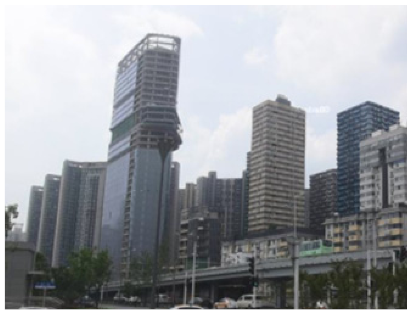 | Central business district (CBD) |
| LCZ 2 compact mid-rise | 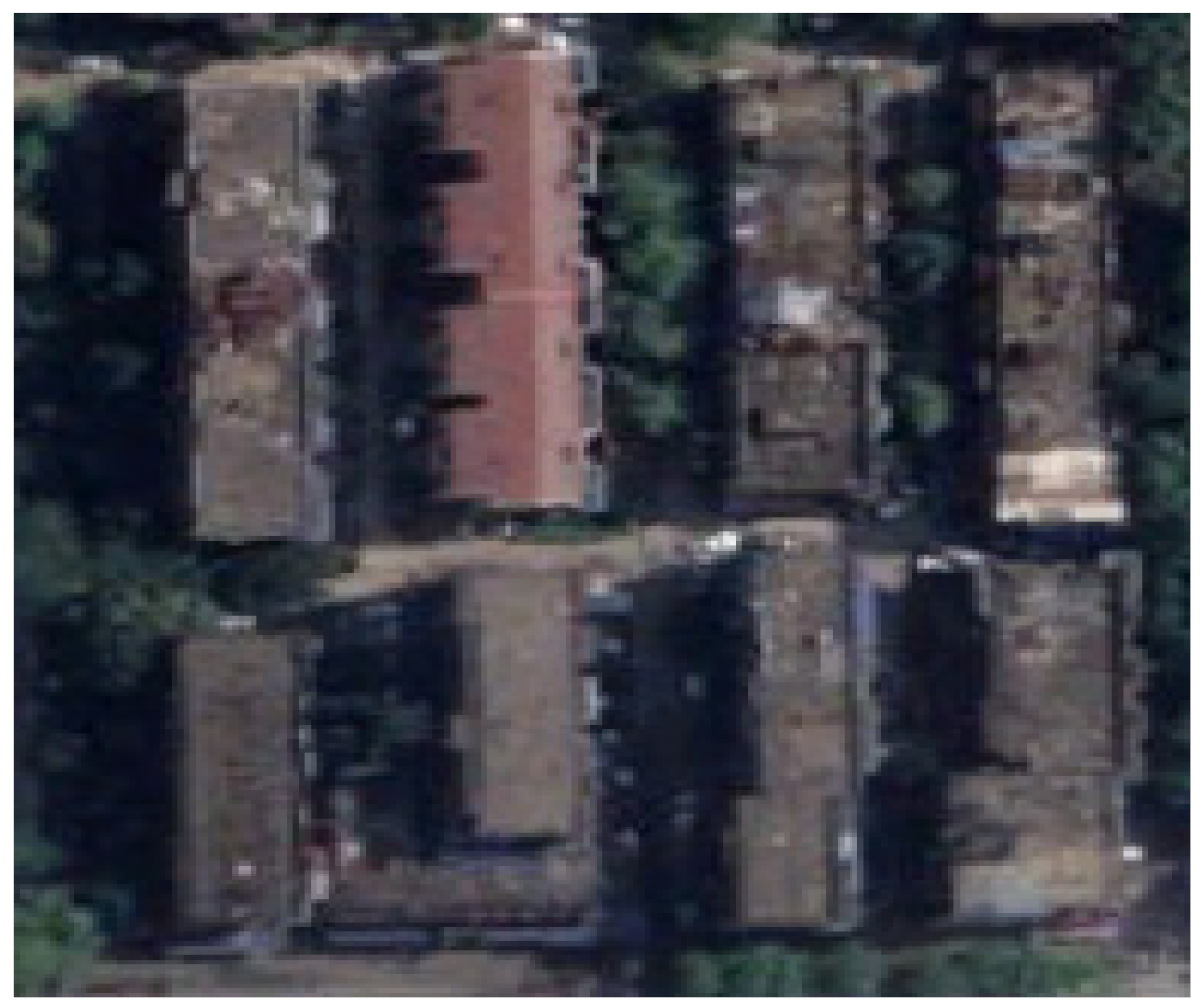 | 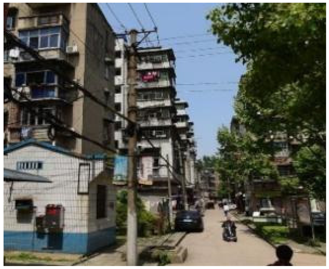 | Old traditional residential area |
| LCZ 3 compact low-rise |  | 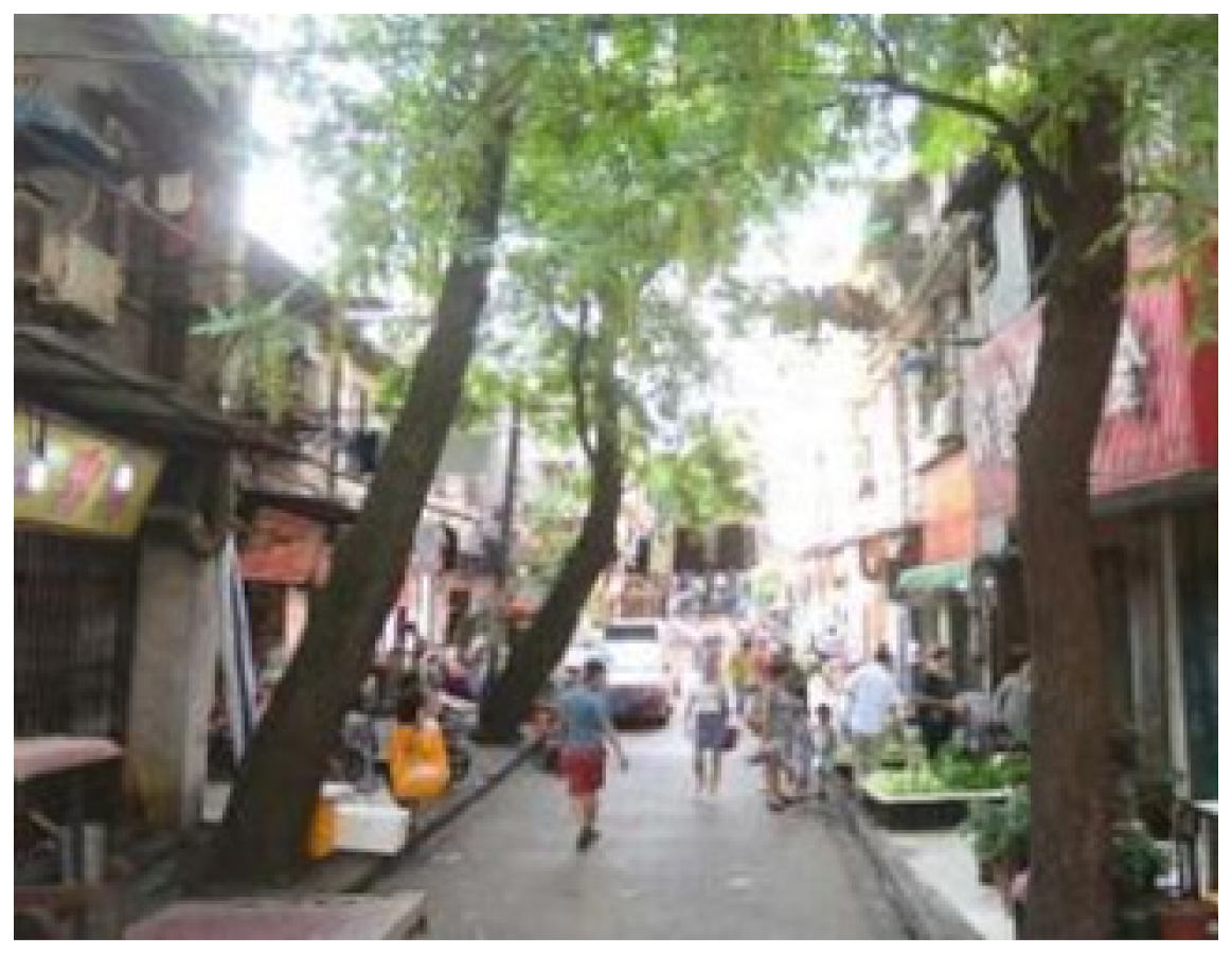 | Urban villages |
| LCZ 4 open high-rise | 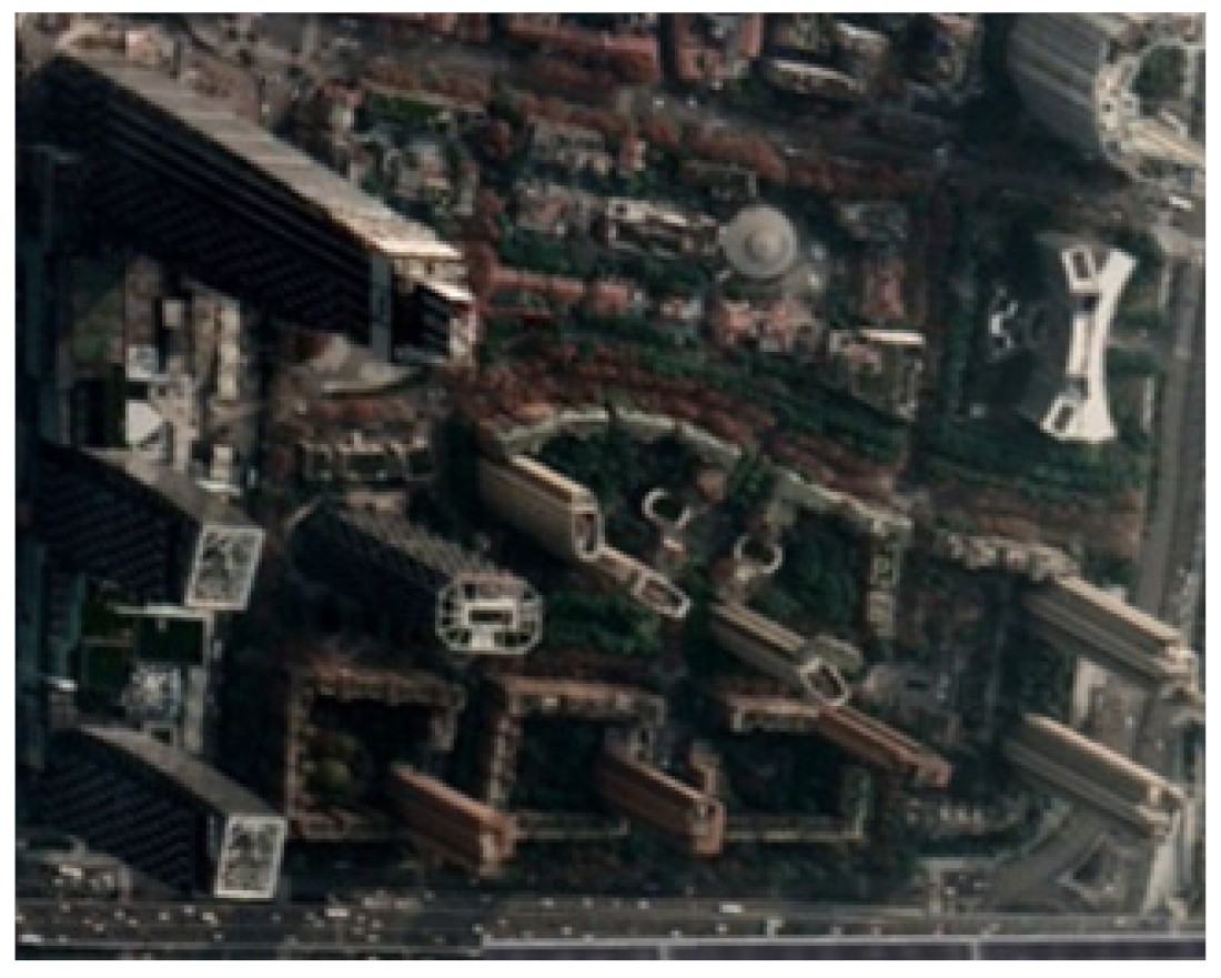 | 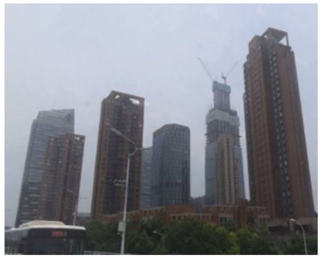 | CBD or high-rise residential building |
| LCZ 5 open mid-rise | 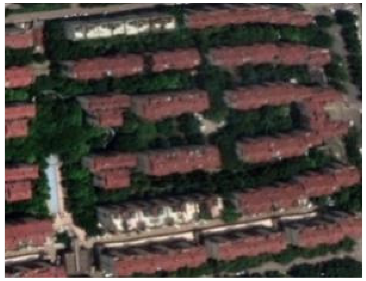 |  | New residential district |
| LCZ 6 open low-rise | 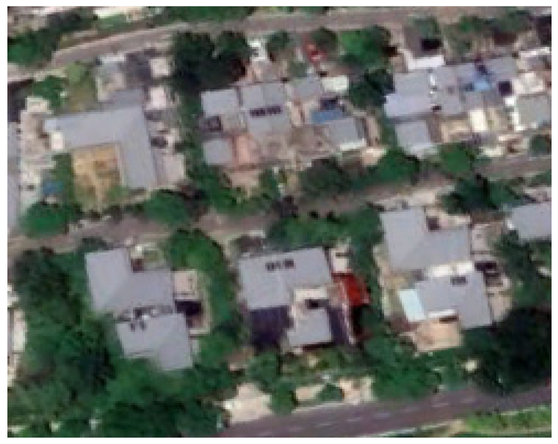 |  | Upscale villas |
| Factors | Summer | Winter |
|---|---|---|
| LCZ | 0.6598 | 0.3159 |
| NDVI | 0.6044 | 0.2844 |
| SAVI | 0.6269 | 0.2844 |
| NDBI | 0.1446 | 0.0956 |
| MNDWI | 0.6408 | 0.2497 |
| POP | 0.5257 | 0.1866 |
| NLI | 0.3548 | 0.0913 |
| RD | 0.1890 | 0.0206 |
Publisher’s Note: MDPI stays neutral with regard to jurisdictional claims in published maps and institutional affiliations. |
© 2022 by the authors. Licensee MDPI, Basel, Switzerland. This article is an open access article distributed under the terms and conditions of the Creative Commons Attribution (CC BY) license (https://creativecommons.org/licenses/by/4.0/).
Share and Cite
Wang, R.; Wang, M.; Zhang, Z.; Hu, T.; Xing, J.; He, Z.; Liu, X. Geographical Detection of Urban Thermal Environment Based on the Local Climate Zones: A Case Study in Wuhan, China. Remote Sens. 2022, 14, 1067. https://doi.org/10.3390/rs14051067
Wang R, Wang M, Zhang Z, Hu T, Xing J, He Z, Liu X. Geographical Detection of Urban Thermal Environment Based on the Local Climate Zones: A Case Study in Wuhan, China. Remote Sensing. 2022; 14(5):1067. https://doi.org/10.3390/rs14051067
Chicago/Turabian StyleWang, Renfeng, Mengmeng Wang, Zhengjia Zhang, Tian Hu, Jiawen Xing, Zhanjun He, and Xiuguo Liu. 2022. "Geographical Detection of Urban Thermal Environment Based on the Local Climate Zones: A Case Study in Wuhan, China" Remote Sensing 14, no. 5: 1067. https://doi.org/10.3390/rs14051067
APA StyleWang, R., Wang, M., Zhang, Z., Hu, T., Xing, J., He, Z., & Liu, X. (2022). Geographical Detection of Urban Thermal Environment Based on the Local Climate Zones: A Case Study in Wuhan, China. Remote Sensing, 14(5), 1067. https://doi.org/10.3390/rs14051067