Abstract
Forest canopy height model (CHM) is useful for analyzing forest stocking and its spatiotemporal variations. However, high-resolution CHM with regional coverage is commonly unavailable due to the high cost of LiDAR data acquisition and computational cost associated with data processing. We present a CHM generation method using U.S. Geological Survey (USGS) 3D Elevation Program (3DEP) LiDAR data for tree height measurement capabilities for entire state of Indiana, USA. The accuracy of height measurement was investigated in relation to LiDAR point density, inventory height, and the timing of data collection. A simple data exploratory analysis (DEA) was conducted to identify problematic input data. Our CHM model has high accuracy compared to field-based height measurement (R2 = 0.85) on plots with relatively accurate GPS locations. Our study provides an easy-to-follow workflow for 3DEP LiDAR based CHM generation in a parallel processing environment for a large geographic area. In addition, the resulting CHM can serve as critical baseline information for monitoring and management decisions, as well as the calculation of other key forest metrics such as biomass and carbon storage.
1. Introduction
Tree height is one of the most important attributes that can be used to assess the ecological status and economic value of a forest system [1] and to estimate ecosystem services it provides, such as carbon sequestration and productivity [2,3]. However, field-based height measurement is labor-intensive and time-consuming, and infeasible when a field site is inaccessible due to terrain conditions, dense vegetation, or man-made barriers. To address these limitations, various research has been conducted to test the feasibility of applying the light detection and ranging (LiDAR) technology as a complement for forest inventory [4,5,6].
LiDAR has been used to map a continuous three-dimensional (3D) structure of the forestland [7] and biomass estimations [8]. With greater point densities than spaceborne LiDAR and broader areal coverage than ground-based LiDAR, airborne LiDAR has been widely used to measure tree height for forest inventory applications [9,10,11,12,13,14]. Figure 1 shows areal coverage and LiDAR point density of previous forest application research. Previous studies demonstrated that airborne LiDAR could provide a high accuracy height measure with an R2 over 0.9 [15,16] and low measurement error within 1.12 ± 0.56 m from an actual height [10,17]. A similar level of accuracy was observed when LiDAR-based height measurement was applied to deciduous and conifer trees when LiDAR density was above 7 points/m2 [3]. However, the accuracy of LiDAR-based height measurement was shown to decrease when LiDAR point density is reduced below 2 points/m2 [18].
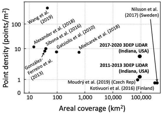
Figure 1.
Areal coverage and point density of airborne LiDAR data.
To date, most studies have been focused on local-level applications of high-density LiDAR data and their spatial extent rarely exceed 1000 km2 (Figure 1). Research on validation of tree LiDAR-based height measurement on a regional scale has been limited due to the cost of LiDAR data acquisition and logistics associated with on-the-ground forest measurement. Although many organizations and agencies have used LiDAR-derived data products for diverse forest management applications, limited peer-reviewed publications are available to formally test the accuracy of LiDAR-derived data products.
Recently, low-density airborne LiDAR data products have become publicly available to support forest management decisions [19,20,21]. In particular, the U.S. Geological Survey (USGS) 3D Elevation Program (3DEP) LiDAR provides wall-to-wall coverage for many states in the USA [22]. Several studies have been conducted to generate forest attributes using the 3DEP LiDAR data [23,24,25]. However, the application of 3DEP LiDAR for large-scale canopy height measurement is still limited due to the large volume of data and relatively insufficient computing power.
We present a canopy height mapping workflow with 3DEP LiDAR across the state of Indiana, USA. To address the issue related to large data size and data processing requirements of 3DEP data, we proposed a stepwise CHM generation framework to produce high-resolution CHMs in an efficient manner. We investigated the accuracy of CHM-based tree height by using tree height collected as part of a field-based forest inventory effort and assessed the accuracy in relation to LiDAR point density and year of data acquisition. The resulting CHMs could be widely applied in the management of timber, fiber, wildlife, and many other disciplines.
2. Materials and Methods
2.1. Forest Inventory Data
The continuous forest inventory (CFI) data used in this study included tree height, inventory year, and geographic location in a total of 4845 plots. Under CFI standards and protocols, tree height is measured as distance from the ground to the highest remaining portion of the tree. All live trees with good form larger than 12.7 cm diameter at breast height (DBH) were measured. For convenient data acquisition, field practitioners commonly used a hypsometer or clinometer to measure tree height and handheld GPS (Allegro handheld computer; Logan, UT, USA) to determine plot location [26]. The difference in GPS measurements over a plot center was calculated and shown in Figure 2. The average and ninety-fifth percentile of the difference in GPS coordinates were 9.0 and 19.7 m. We used forest inventory data collected in 2008–2017.
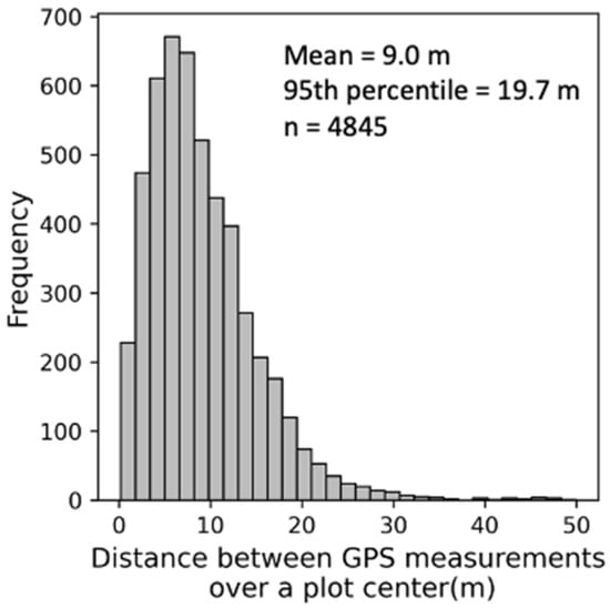
Figure 2.
Distance between GPS measurements over a plot center.
2.2. LiDAR and Digital Terrain Model (DTM) Data
An objective of the 3DEP LiDAR project is to obtain full national coverage with a specific quality level defined by The National Enhanced Elevation Assessment (NEEA) with less than eight years between each cycle (Table A1) [22]. As of 2021, two sets of Indiana’s statewide 3DEP LiDAR data were made available for public access. The first Indiana statewide LiDAR dataset was produced during 2011–2013 with 1.0 or 1.5 m average post spacing. The post spacing is defined as the smallest distance between two points that can be explicitly represented in a gridded elevation dataset [27]. The second statewide LiDAR data in Indiana was acquired during 2017–2020. The average post spacing for this dataset has not been reported in detail, but IGIC (Indiana Geographic Information Council) reported that nominal pulse density is over 2.0 pulses/m2 [28].
For the two statewide LiDAR datasets in Indiana, the bare-earth hydro-flattened digital elevation model (DEM) was also publicly available and used as input data in this study. For brevity, we used the term digital terrain model (DTM) instead of bare-earth hydro-flattened DEM in the rest of the paper. The spatial resolution of DTM is 1.524 m for 2011–2013 LiDAR data and 0.762 m for 2017–2020 LiDAR data. The original 3DEP LiDAR and DTM data are delivered in an individual 1524-by-1524-m tile (Indiana State Plane East/West coordinate system). It should be noted that the unit of length used for 3DEP LiDAR and DTM was originally U.S. survey foot (1 ft = 0.3048 m), and the size of DTM tile corresponds to 1000-by-1000 pixels and 2000-by-2000 pixels for the first and second 3DEP LiDAR project. Data size of LiDAR and DTM was 4.9 and 0.5 terabyte for 2011–2013 3DEP data and 13.0 and 0.7 terabyte for 2017–2020 3DEP data. A total of 42,539 and 48,602 tiled datasets were available for 2011–2013 and 2017–2020 3DEP data.
2.3. Canopy Height Model (CHM) Generation
The CHM is a raster representation of the distance from the ground surface to the highest canopy structure of vegetation. A simplified CHM generation procedure was summarized as follows: creating a normalized digital surface model (nDSM) and CHM (Figure 3). First, an nDSM was created by calculating the distance between DTM and the highest z value of the LiDAR points in each pixel. Second, CHM was created by suppressing height as zero on non-forested area.
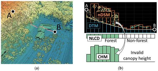
Figure 3.
A subset of (a) 3D Elevation Program (3DEP) LiDAR data from Martell Forest in Indiana, USA with (b) a 2D slice of point cloud along the transect from point A to B showing the canopy height model (CHM) generation procedure. nDSM: normalized digital surface model, DTM: digital terrain model, NLCD: National Land Cover Database-based binary classification map of forested and non-forested areas, and CHM: canopy height model.
The individual nDSM tiles were generated by the following procedure (Figure 4). First, tiled LiDAR point cloud and DTM were loaded. LiDAR points that are not earth-bound, e.g., birds, and erroneous, and spurious, i.e., elevation error near water-ground interface, were excluded in the CHM generation process [22]. The noisy LiDAR points were identified by data vendors prior to 3DEP data publishing. Second, nDSM raster with 1.524 m spatial resolution was initialized with zero normalized height in the entire tile boundary. Third, nDSM pixel value was iteratively updated for every valid LiDAR point. For each i-th LiDAR point, x, y, and z coordinates; image coordinates m, n in 2-D nDSM array; and average ground elevation (DTMm,n) were obtained. Subsequently, the nDSM pixel value was updated when the normalized height (nHt = z − DTMm,n) was higher than previously assigned nDSMm,n.
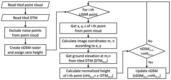
Figure 4.
A workflow to generate the tiled normalized digital surface model (nDSM) using 3D Elevation Program (3DEP) LiDAR and digital terrain model (DTM) data. nHt: normalized height.
Tiled nDSM data were combined to generate a countywide CHM (Figure 5). All nDSM tiles with 1.524 m spatial resolution in a county were merged and clipped by the county boundary polygon. Normalized height in non-forestland was changed to the invalid value using the 2013 and 2019 National Land Cover Database (NLCD)-derived forested and non-forested classification map [29]. A temporary upscaled NLCD land cover map was generated to match the spatial resolution of the input nDSM with a nearest neighbor sampling method. We used a common spatial reference system for the CHM data products with the Universal Transverse Mercator (UTM) coordinate system (zone 16N) for the output CHMs. The entire CHM generation process was implemented using the Geospatial Data Abstraction Library (GDAL) package with Python programming language.
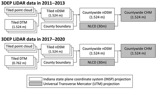
Figure 5.
A workflow to generate countywide canopy height models (CHM) using 3D Elevation Program (3DEP) LiDAR data.
We used a high-performance computer (HPC) and parallel processing to efficiently produce the high-resolution CHM dataset. The USGS 3DEP datasets of approximately 20 terabytes in size were stored in a network-attached storage (NAS) device of 100 terabyte storage capacity (Synology Inc., Taiwan). The original data were sequentially copied to an HPC file system, and copied data were used to generate tiled nDSM using an HPC node (two 2.0 GHz AMD Rome CPUs, 256 gigabyte RAM) (Figure 6). We distributed the identical nDSM generation tasks with different tiled datasets using a task parallelism design since individual tasks do not depend on outcomes from other tasks. The output nDSM was moved to the NAS device once each processing task was complete. The countywide CHM was created by merging nDSMs on a single node workstation (Intel Xeon CPU, E5–2687W @ 3.40 GHz, 32 gigabyte RAM).
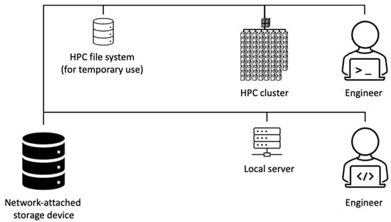
Figure 6.
Data storage and canopy height model processing architecture for 3D Elevation Program LiDAR data in Indiana.
2.4. Accuracy Assessment of LiDAR-Based Height Measurement
The accuracy of LiDAR-based height was validated by comparing height metrics obtained from inventory and LiDAR data in the plot area. We used maximum and average tree height as inventory height metrics. LiDAR height measurements including percentiles and an average of elevation was obtained after subtracting ground elevation from LiDAR z values. Points greater than 2 m above ground was selectively used to obtain average LiDAR height. Additionally, the maximum CHM was obtained as a LiDAR height metric (Figure 7).
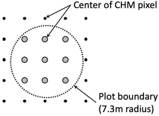
Figure 7.
Extraction of plot-level maximum tree height using canopy height model (CHM). The maximum canopy height was derived by searching inside a continuous forest inventory (CFI) plot area (r = 7.32 m).
We validated height accuracy using a pair of inventory and LiDAR metrics with the highest correlation coefficient. The correlation between maximum CHM and LiDAR height was shown to investigate whether the raster-based maximum height can be used instead of maximum LiDAR height. We used multiple plot radii to clip spatial data (3.7, 7.3, 11.0, and 14.6 m) to investigate whether the size of the clipping area affects the correlation between the inventory height and LiDAR height metrics.
Height measurement accuracy was evaluated by examining the difference between LiDAR and inventory height. The height difference was assessed according to LiDAR point density, inventory height, LiDAR data acquisition year, inventory year, and year difference between LiDAR and inventory data collection to identify potential sources of error.
A supplementary height validation was conducted on forest plots with a lower positional difference between GPS measurements. The purpose of this validation was to evaluate measurement accuracy on forest plots when co-registration between LiDAR data and inventory information was accurate. Inventory plots in Yellowwood State Forest (YSF), Indiana, USA, were chosen for ease of access to densely located forest plots. We remeasured geolocations of metal stakes at plot centers in YSF area using Trimble Juno (Sunnyvale, CA, USA) and calculated 2D distance between previous and remeasured GPS coordinates. Inventory plots were excluded in the validation if the 2D distance error was larger than 0.1 m [8].
3. Results
3.1. Canopy Height Model (CHM)
The CHM was created from 2011–2013 and 2017–2020 3DEP LiDAR data at the designated spatial resolutions (Figure 5 and Figure 8). The average and standard deviation of pixel-wise canopy height was 18.2 and 8.1 m. The visualization and download of LiDAR data products are available as a web service [30,31].

Figure 8.
Visualization of (a) canopy height model (CHM) of Indiana, USA, (b) CHM in Tippecanoe County, Indiana, USA, and (c) CHM in Martell Forest in Tippecanoe County, Indiana, USA.
Estimated processing time for the Indiana statewide LiDAR data was approximately 60 h. Most of the processing time was spent producing tiled nDSM with an average processing time of 28.4 s per tile (91,141 tiles in total) (Figure 4). The entire nDSM generation tasks performed by HPC resulted in an estimated processing time of 60 h (28.4 sec⋅core/tiled dataset × 91,141 tiled datasets/12 cores/3600 s/h = 60 h). Time spent transferring data between the server and HPC file system could not be accurately measured due to the fluctuation of network speed or network connectivity issues. However, a data transfer rate of 15 megabyte per second was generally enough to avoid idle time between the consecutive nDSM processing tasks. The countywide CHM generation of 92 Indiana counties took approximately 1 h from the standalone server.
3.2. Correlation between Inventory and LiDAR Height Metrics
LiDAR height metrics generally showed a moderate to strong correlation with maximum inventory height (Figure 9 and Figure 10). Correlation between maximum inventory height and maximum LiDAR height was in 0.91 for the 2011–2013 LiDAR data and 0.84 for the 2017–2020 data when the positional difference of plot center was less than 0.1 m. Correlation between maximum inventory height and LiDAR percentile height had a negative trend as the percentile number decreased. Average LiDAR height and maximum inventory height had a correlation coefficient less than 0.75.
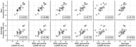
Figure 9.
Correlation between LiDAR and inventory height metrics. LiDAR data in 2011–2013 and inventory data in 2008–2012 were used. Forest plots have positional uncertainty approximately less than 0.1 m (n = 25). Ht: height.
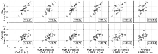
Figure 10.
Correlation between LiDAR and inventory height metrics. LiDAR data in 2017–2020 and inventory data in 2013–2017 were used. Forest plots have positional uncertainty approximately less than 0.1 m (n = 24). Ht: height.
Average inventory height and LiDAR height metrics had less positive correlation coefficients between 0.4–0.8. The ninety-ninth percentile of LiDAR height had the strongest correlation of 0.78 and 0.76. A decreasing trend of correlation coefficients between average inventory height and LiDAR height percentiles was observed as percentile number decreased. Correlation between average LiDAR height and average inventory height was 0.6. We also conducted correlation analysis between median inventory height and LiDAR metrics. However, we do not report the result since the correlation was weaker than the above results.
The correlation analysis showed that the maximum inventory height was most highly correlated with maximum LiDAR heights. Therefore, we used the term inventory height and LiDAR height in the rest of the paper to indicate maximum inventory and LiDAR height.
The size of the clipping area used to obtain LiDAR height did not show a significant effect on the correlation of LiDAR and inventory height (Table 1). Slightly higher correlation coefficients were observed when the clipping radius was either 7.3 or 11.0 m. However, the correlation coefficients did not improve more than 0.1 within the studied range of clipping radius from 3.7 to 14.6 m. Therefore, we used a clipping radius of 7.3 m, i.e., radius of inventory plot, in the rest of the paper to obtain LiDAR height. A substantial difference in the correlation coefficient was shown according to the positional difference of plot location. A higher correlation of 0.8 was observed when the positional difference of the plot was less than 0.1 m.

Table 1.
Effect of clipping area (radius) and positional difference of plot center location on correlation between LiDAR and inventory height. LiDAR height was obtained from a circular area with variable radii, whereas inventory height was acquired within the original plot area with a 7.3 m radius.
A very strong correlation of 0.95 was observed between LiDAR and CHM-based height (Figure 7) from the entire set of inventory plots. Consequently, plot-wise LiDAR tree height was obtained from CHM henceforth, and we refer to it as CHM height.
3.3. An Accuracy Assessment of CHM-Based Height
The average and standard deviation of inventory tree height were 27.5 and 5.9 m from 4845 forest plots. The corresponding statistics obtained by CHM were 28.2 and 5.6 m, respectively. It should be noted that above statistics are plot-wise maximum tree height, whereas the statistics in Section 3.1 were calculated from pixel-wise canopy height.
3.3.1. Effect of LiDAR Point Density on Height Accuracy
Average and standard deviation of LiDAR density were 1.6 and 1.1 points/m2 for 2011–2013 LiDAR and 6.0 and 3.2 points/m2 for 2017–2020 LiDAR data. Height error in relation to LiDAR point density mostly showed a positively skewed distribution (Figure 11). Median values were in a −3 to 5 m range. However, height error had a negatively skewed distribution for 2017–2020 LiDAR data when LiDAR point density was under 4 points/m2. The third percentile of error distribution was −31 m when point density was 0–2 points/m2 and −20 m when point density was 2–4 points/m2.
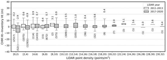
Figure 11.
Height measurement error with respect to LiDAR point density. Boundaries of upper and lower whisker are the ninety-seventh and third percentiles. The number above each box plot is median, and the number below box plot is number of data points. CHM: canopy height model; Ht: height.
Height measurement error was displayed with respect to LiDAR acquisition year to investigate whether the data acquired in a specific year caused a larger error (Figure 12). The result showed that measurement error was mostly positively skewed for all data acquisition years. However, the height errors obtained from 2018 LiDAR data were negatively skewed when point density was 0–4 points/m2. The errors from 2018 LiDAR data had a distinctively longer lower whisker when the point density values were under 2 points/m2.
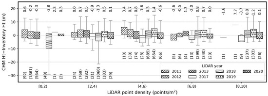
Figure 12.
Height measurement error in relation to LiDAR point density and acquisition year. Data with LiDAR density less than 10 points/m2 were displayed. Boundaries of upper and lower whisker is the ninety-seventh and third percentiles. The number above each box plot is median, and the number below box plot is number of data points. CHM: canopy height model; Ht: height.
3.3.2. Effect of Tree Height on Measurement Accuracy
Height measurement error generally showed a decreasing trend as tree height increased (Figure 13). The variance of error also decreased as tree height increased. Standard deviation of height error was 10.0 m when tree height was in the 6–9 m range and 3.6 m when tree height was in the 39–42 m range. In particular, the height error calculated from the 2018 LiDAR data showed more negatively skewed distribution compared to other LiDAR acquisition years.
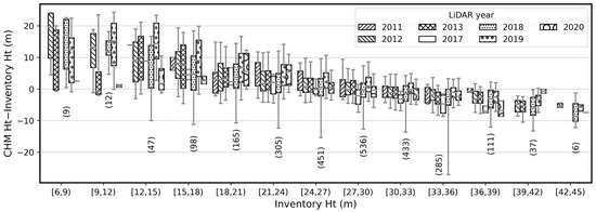
Figure 13.
Height measurement error with respect to inventory height and LiDAR data acquisition year. Boundaries of upper and lower whisker is the 97th and 3rd percentiles. The number below box plot is number of data points of 2018 LiDAR data. CHM: canopy height model; Ht: height.
3.3.3. Effect of Data Acquisition Timing on Measurement Accuracy
The time difference between field inventory and LiDAR data acquisition did not significantly affect the overall height measurement error (Figure 14). However, the height measured by LiDAR data was generally overestimated when LiDAR data were collected five or more years after the collection of field inventory data. Height measurement error had a median value of 0.7 m when the time difference was five years and 2.1 m when the time difference was 6–7 years. We observed height error in relation to the combination of LiDAR and inventory year, which did not show a noticeable trend (Figure 15). However, height error calculated from the 2018 LiDAR data again showed a larger variance with significant underestimation compared to other LiDAR data collection years.
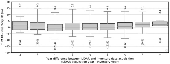
Figure 14.
Height measurement error with respect to time difference between inventory and LiDAR data acquisition. Boundaries of upper and lower whisker is the ninety-seventh and third percentiles. The number above each box plot is median, and the number below box plot is number of data points. CHM: canopy height model; Ht: height.
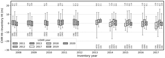
Figure 15.
Height measurement error with respect to inventory and LiDAR acquisition year. Boundaries of upper and lower whisker is the ninety-seventh and third percentiles. The number above each box plot is median, and the number below box plot is number of data points. CHM: canopy height model; Ht: height.
3.3.4. Height Accuracy When Accurate Location Is Provided
From the inventory plots which had positional difference less than 0.1 m, CHM height showed a strong correlation with on-the-ground measurements (Figure 16). Canopy height observed from 2011 and 2017 LiDAR data resulted in R2 values of 0.92 and 0.85, respectively. Root mean square error (RMSE) of height measurement was 2.7 m with 2011 LiDAR and 3.5 m with 2017 LiDAR data. The regression lines of the two datasets had a slope under 1.0 and an intercept of approximately 10 m. Comparison of CHM and field-based height measurements with the entire set of inventory plots in the state of Indiana resulted in a lower R2 and higher RMSE value (Figure A1).
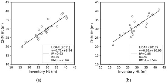
Figure 16.
Agreement between inventory and canopy height when positional uncertainty was under approximately 0.1 m: (a) LiDAR measurement in 2011 and field measurement in 2009–2010, (b) LiDAR measurement in 2017 and field measurement in 2014–2015. CHM: canopy height model, Ht: height.
4. Discussion
Our study presented a CHM generation and validation framework based on USGS 3DEP LiDAR. The proposed CHM generation workflow is specifically designed to process large LiDAR dataset in a parallel processing environment (Figure 4, Figure 5 and Figure 6). The CHM generation process can be applied to other LiDAR datasets with a local or regional coverage. Likewise, the plot-level accuracy assessment approach can be applied to other inventory plots with a different design.
This study demonstrated that canopy height obtained from 3DEP LiDAR has a strong correlation to inventory height (Figure 9, Figure 10 and Figure 16). This result is consistent with previous findings that airborne LiDAR is a reliable technique to obtain heights of upper canopy trees, i.e., dominant and co-dominant trees [19]. We generated CHM using LiDAR points with maximum elevation (Figure 3) in a 1.524-by-1.524-m pixel area. Correspondingly, we compared plot-wise maximum inventory height and maximum CHM height for the accuracy assessment. The selection of inventory and LiDAR height metrics were based upon the correlation analysis of multiple LiDAR and inventory height metrics (Figure 9 and Figure 10). However, previous studies suggest that height percentiles or other forest structural metrics can be used to predict tree height metrics such as dominant height, bole height, or Lorey’s height [32,33].
The error of CHM-based height measurement generally had a consistent distribution in relation to LiDAR point density and inventory year (Figure 11, Figure 12, Figure 14 and Figure 15). However, areas with low-density LiDAR data acquired in 2018 resulted in an underestimation of canopy height (Figure 11). From a total of 1132 inventory plots which had point density of 0–4 points/m2 from 2018 LiDAR data, the average and standard deviation of height error was −2.1 m and 7.7 m. The number of plots with a height underestimation below two standard deviations from the average was 61 (61/1132 = 5%). The outlier plots were found at a specific region in Southeastern Indiana (mostly in Clark, Jackson, Washington, Jennings County) (Figure 17). It was revealed that these plots were distributed along the region with a lower LiDAR density in the 2017–2020 LiDAR data. The repeated pattern of darker vertical strips in CHM occurred because point density below the sensor flight line (headed north or south) was lower compared to areas covered by multiple scans where the LiDAR sensor was headed north and south. The CHM pixels with a fewer number of canopy returns were widespread in the low-density strips. We believe that the lower density strips and resulting height error can primarily be attributed to the configuration of LiDAR data collection at specific locations rather than the actual variations in canopy structure (Figure 17c,d). Possible causes of these low LiDAR density strips could be LiDAR sensor configuration, low flight altitude, unexpected weather, or abrupt aircraft maneuvers, and should be further investigated.
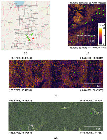
Figure 17.
Inventory plots (green dots) with low height measurement accuracy: (a) plots with low height accuracy located in southeastern Indiana; (b) a subset of plots on top of canopy height model (CHM) from 2017–2020 LiDAR data, plots with low height accuracy distributed along the banded regions with a lower LiDAR point density (Figure 12); (c) CHM of dotted area in (b); (d) 2018 National Agriculture Image Program (NAIP) County Mosaic image of dotted area in (b). Ht: height. Note: a majority of inventory plots with an error less than two standard deviations were not displayed for brevity.
An interesting trend was revealed between tree height underestimation and LiDAR point density (Figure 18). It was shown that the magnitude of the largest negative height error was associated with the proportion of inventory plots with LiDAR density between 0–4 points/m2 per county. In other words, counties with higher LiDAR density were less prone to severe height underestimation. It should be noted that the values of the y axis in Figure 18 are minimum values of height measurement error.
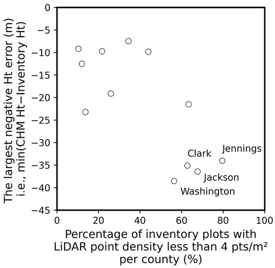
Figure 18.
The largest negative height measurement error with respect to the proportion of inventory plots in counties with low LiDAR point density (0–4 points/m2). Data include Indiana counties where 3D Elevation Program (3DEP) LiDAR data was collected in 2018. Counties having 20 or less inventory plots were excluded to highlight a statistical trend. Southeast Indiana counties with a large negative error (Figure 17a) were labeled.
The CHM of Southeastern Indiana counties should be carefully used when measuring canopy height since it can underestimate actual height value (Figure 12, Figure 17 and Figure 18). Height accuracy can particularly decrease on areas without a LiDAR return (initialized with zero in our case) or areas with lower point density. One can create a CHM with a larger pixel size by assigning maximum canopy height in each pixel area, or one can interpolate nearby valid canopy height can reduce the error. The accuracy of plot-wise canopy height can be minimally affected unless the highest tree is located near a plot boundary or a pixel boundary.
Tree height was heavily overestimated up to approximately 20 m when inventory height was under 12 m (Figure 13). The overestimation could have occurred when the geolocation of the plot center was not accurate or when large trees with 12.7 cm or less in diameter were not included in measurement due to the CFI protocol.
The main challenge in comparing the tree height using the CFI and CHM data was the positional error of GPS coordinates in plot center measurement (Figure 2, Figure 16 and Figure A1). The ninetieth percentile of positioning error of common handheld GPS devices was previously reported as 13.1 m in high forest [34]. The GPS error under a tree canopy increases due to unfavorable satellite constellation geometry, atmospheric interference, multi-path effect, and lower signal-to-noise ratio [35,36]. Since the positioning error can far exceed the inventory plot radius (7.3 m), it is possible that there is minor or no overlap between an actual and a nominal plot area in extreme cases.
Inventory plots with positional difference within 0.1 m were selectively used to mitigate co-registration issue between geospatial data (LiDAR) and plot center location. A more rigorous accuracy assessment would have been possible if accurate GPS remeasurements on plot centers were available across the state. However, the criteria used to select the inventory plots could still result in a biased set of evaluation points because the accuracy issues with GPS measurement were not completely eradicated. The positional uncertainty issue can be potentially alleviated if the plot centers are measured using a high-precision GPS device with real-time kinematic (RTK), post-processed kinematic (PPK) positioning, networked transport of RTCM via internet protocol (NTRIP) correction, or by other precision surveying techniques. If the issue with positional accuracy is resolved, diverse studies regarding the relationships between forest inventory attributes and remote sensing data can be conducted.
We conducted accuracy assessment based on point density (points/m2). However, it is more desirable to use pulse density since it is less affected by characteristics of targets and more dependent on sensor configuration. Pulse density of multiple return LiDAR data can be computed by counting the number of the first returns in unit area.
The characteristics of LiDAR and foliage density could adversely affect the accuracy of tree height measurement. A tree with a low foliage density can cause LiDAR pulse to travel a longer distance before being reflected at a thick branch or trunk. The effect of low-density foliage can be intensified when the data collection is done during leaf-off season. However, point density over 4 points/m2 was considered sufficient to measure hardwood trees with a height over 25 m consistently (Figure 13). As USGS increases its LiDAR data acquisition effort to higher densities (8 pulses/m2), point densities of future 3DEP LiDAR data will likely also increase.
There are other factors that could also affect the accuracy of tree height measurement. First, a human error could be introduced while measuring height in the field. When collecting inventory data across a large geographic region, the “time window” allowed for data acquisition is relatively small, especially in areas where there are large elevation gradients like in the western USA. Long data collection period for large areas can often lead to multi-year and multi-vendor contracts, causing potential complications in project management and inconsistencies in data attributes and quality. Second, tree canopy structures originating from outside a plot boundary, i.e., over-hanging branches, can cause an overestimation in tree height measurement. Third, our DTM-based nDSM generation method can produce a discontinuous CHM over a smooth canopy surface when the terrain slope is rugged. The discontinuous CHM can occur when a single ground height is assigned within the entire 1.524-by-1.524-m pixel area of DTM (Figure 3). Conversely, a continuous terrain model derived by mesh or triangulated irregular network (TIN) can be used to model more smooth ground surface [37]. Fourth, an airborne LiDAR data has its own source of error, such as sensor position, GPS-IMU integration, signal attenuation by the atmosphere, divergence of laser footprint, and aircraft vibration. However, the amount of the LiDAR error (Table A1) is considered relatively small compared to that of the other causes. Fifth, a more rigorous filtering algorithm can be used to remove spurious LiDAR returns.
5. Conclusions
This study presented a CHM generation workflow using USGS 3DEP LiDAR data which is characterized by a low-density point cloud and a large spatial coverage. We designed an efficient CHM generation workflow that enables parallel processing to address the issue of large data size of 3DEP data. We investigated accuracy of CHM-based height measurement according to point density and inventory height, and suggested an exploratory data analysis (EDA) approach to find problematic input data. The accuracy assessment of tree height demonstrated that the LiDAR-based CHM contains reliable height information. It is expected that this study could facilitate the use of USGS 3DEP data for the evaluation of forest conditions and ecosystem services in other regions.
Author Contributions
Conceptualization, J.J. and S.F.; methodology, S.O., J.J., G.S. (Guofan Shao), G.S. (Gang Shao) and S.F.; validation, S.O., J.J. and S.F.; formal analysis, S.O.; investigation, S.O., J.J., G.S. (Guofan Shao) and S.F.; resources, J.J. and S.F.; data curation, S.O., J.J., G.S. (Gang Shao), J.G. and S.F.; writing—original draft preparation, S.O., J.J., G.S. (Guofan Shao) and S.F.; writing—review and editing, S.O., J.J., G.S. (Guofan Shao), G.S. (Gang Shao) and S.F.; visualization, S.O.; supervision, J.J., G.S. (Guofan Shao) and S.F.; project administration, J.J. and S.F.; funding acquisition, J.J. and S.F. All authors have read and agreed to the published version of the manuscript.
Funding
This work was supported by the Hardwood Tree Improvement and Regeneration Center and the USDA Forest Service (#19-JV-11242305-102) and the USDA National Institute of Food and Agriculture McIntire Stennis project (IND011523MS). The research is partially supported by the Purdue Integrated Digital Forestry Initiative and by USDA Forest Service (Grant No. 19-JV-11242305-102).
Institutional Review Board Statement
Not applicable.
Informed Consent Statement
Not applicable.
Acknowledgments
A sincere thank you to Rebekah Shupe for her proofreading of this paper.
Conflicts of Interest
The authors declare no conflict of interest.
Appendix A

Table A1.
Minimum requirements (quality level 2, QL2) of 3D Elevation Program (3DEP) LiDAR products.
Table A1.
Minimum requirements (quality level 2, QL2) of 3D Elevation Program (3DEP) LiDAR products.
| Requirements | Range |
|---|---|
| Aggregate nominal pulse spacing (m) | ≦0.71 |
| Aggregate nominal pulse density (pulses/m2) | ≧2.0 |
| Smooth surface repeatability, RMSD * (m) | ≦0.06 |
| Swath overlap difference, RMSD (m) | ≦0.08 |
| RMSE (non-vegetated, m) | ≦0.1 |
| Non-vegetated vertical accuracy at 95% confidence level (m) | ≦0.196 |
| Vegetated vertical accuracy at the 95% confidence level (m) | ≦0.30 |
* RMSD is the root mean square deviation and calculated as the root mean square error (RMSE). RMSD is used when there is no independent data source with higher accuracy.
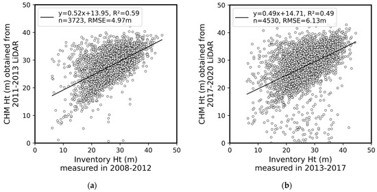
Figure A1.
Agreement between inventory and canopy height from the entire set of inventory plots: (a) LiDAR measurement in 2011–2013 and field measurement in 2008–2012, (b) LiDAR measurement in 2017–2020 and field measurement in 2013–2017. Inventory plots without valid height measurement were excluded from the scatter plots. CHM: canopy height model, Ht: height.
References
- Leites, L.P.; Robinson, A.P.; Crookston, N.L. Accuracy and Equivalence Testing of Crown Ratio Models and Assessment of Their Impact on Diameter Growth and Basal Area Increment Predictions of Two Variants of the Forest Vegetation Simulator. Can. J. For. Res. 2009, 39, 655–665. [Google Scholar] [CrossRef]
- Brando, P. Tree Height Matters. Nat. Geosci. 2018, 11, 390–391. [Google Scholar] [CrossRef]
- Stereńczak, K.; Mielcarek, M.; Wertz, B.; Bronisz, K.; Zajączkowski, G.; Jagodziński, A.M.; Ochał, W.; Skorupski, M. Factors Influencing the Accuracy of Ground-Based Tree-Height Measurements for Major European Tree Species. J. Environ. Manag. 2019, 231, 1284–1292. [Google Scholar] [CrossRef] [PubMed]
- Bouvier, M.; Durrieu, S.; Fournier, R.A.; Renaud, J.P. Generalizing Predictive Models of Forest Inventory Attributes Using an Area-Based Approach with Airborne LiDAR Data. Remote Sens. Environ. 2015, 156, 322–334. [Google Scholar] [CrossRef]
- Gray, A.; Brandeis, T.; Shaw, J.; McWilliams, W.; Miles, P. Forest Inventory and Analysis Database of the United States of America (FIA). Biodivers. Ecol. 2012, 4, 225–231. [Google Scholar] [CrossRef] [Green Version]
- Wallace, L.; Lucieer, A.; Watson, C.; Turner, D. Development of a UAV-LiDAR System with Application to Forest Inventory. Remote Sens. 2012, 4, 1519–1543. [Google Scholar] [CrossRef] [Green Version]
- Larue, E.A.; Hardiman, B.S.; Elliott, J.M.; Fei, S. Structural Diversity as a Predictor of Ecosystem Function. Environ. Res. Lett. 2019, 14, 114011. [Google Scholar] [CrossRef]
- Shao, G.; Shao, G.; Gallion, J.; Saunders, M.R.; Frankenberger, J.R.; Fei, S. Improving Lidar-Based Aboveground Biomass Estimation of Temperate Hardwood Forests with Varying Site Productivity. Remote Sens. Environ. 2018, 204, 872–882. [Google Scholar] [CrossRef]
- Alexander, C.; Korstjens, A.H.; Hill, R.A. Influence of Micro-Topography and Crown Characteristics on Tree Height Estimations in Tropical Forests Based on LiDAR Canopy Height Models. Int. J. Appl. Earth Obs. Geoinf. 2018, 65, 105–113. [Google Scholar] [CrossRef]
- Andersen, H.E.; Reutebuch, S.E.; McGaughey, R.J. A Rigorous Assessment of Tree Height Measurements Obtained Using Airborne Lidar and Conventional Field Methods. Can. J. Remote Sens. 2006, 32, 355–366. [Google Scholar] [CrossRef]
- Barnes, C.; Balzter, H.; Barrett, K.; Eddy, J.; Milner, S.; Suárez, J.C. Remote Sensing Individual Tree Crown Delineation from Airborne Laser Scanning for Diseased Larch Forest Stands. Remote Sens. 2017, 9, 231. [Google Scholar] [CrossRef] [Green Version]
- Bottalico, F.; Chirici, G.; Giannini, R.; Mele, S.; Mura, M.; Puxeddu, M.; Mcroberts, R.E.; Valbuena, R.; Travaglini, D. Modeling Mediterranean Forest Structure Using Airborne Laser Scanning Data. Int. J. Appl. Earth Obs. Geoinf. 2017, 57, 145–153. [Google Scholar] [CrossRef]
- González-Ferreiro, E.; Diéguez-Aranda, U.; Barreiro-Fernández, L.; Buján, S.; Barbosa, M.; Suárez, J.C.; Bye, I.J.; Miranda, D. A Mixed Pixel-and Region-Based Approach for Using Airborne Laser Scanning Data for Individual Tree Crown Delineation in Pinus Radiata D. Don Plantations. Int. J. Remote Sens. 2013, 34, 7671–7690. [Google Scholar] [CrossRef]
- Mohan, M.; Araujo, B.; de Mendonça, F.; Silva, C.A.; Klauberg, C.; Santos De Saboya Ribeiro, A.; Gomes De Araújo, E.J.; Monte, M.A.; Cardil, A. Optimizing Individual Tree Detection Accuracy and Measuring Forest Uniformity in Coconut (Cocos Nucifera L.) Plantations Using Airborne Laser Scanning. Ecol. Model. 2019, 409, 108736. [Google Scholar] [CrossRef]
- Mielcarek, M.; Stereńczak, K.; Khosravipour, A. Testing and Evaluating Different LiDAR-Derived Canopy Height Model Generation Methods for Tree Height Estimation. Int. J. Appl. Earth Obs. Geoinf. 2018, 71, 132–143. [Google Scholar] [CrossRef]
- Sibona, E.; Vitali, A.; Meloni, F.; Caffo, L.; Dotta, A.; Lingua, E.; Motta, R.; Garbarino, M. Direct Measurement of Tree Height Provides Different Results on the Assessment of LiDAR Accuracy. Forests 2017, 8, 7. [Google Scholar] [CrossRef]
- Gatziolis, D.; Fried, J.S.; Monleon, V.S. Challenges to Estimating Tree Height via LiDAR in Closed-Canopy Forests: A Parable from Western Oregon. For. Sci. 2010, 56, 139–155. [Google Scholar] [CrossRef]
- Kwak, D.A.; Lee, W.K.; Lee, J.H.; Biging, G.S.; Gong, P. Detection of Individual Trees and Estimation of Tree Height Using LiDAR Data. J. For. Res. 2007, 12, 425–434. [Google Scholar] [CrossRef]
- Kotivuori, E.; Korhonen, L.; Packalen, P. Nationwide Airborne Laser Scanning Based Models for Volume, Biomass and Dominant Height in Finland. Silva Fenn. 2016, 50, 1567. [Google Scholar] [CrossRef] [Green Version]
- Moudrý, V.; Urban, R.; Štroner, M.; Komárek, J.; Brouček, J.; Prošek, J. Comparison of a Commercial and Home-Assembled Fixed-Wing UAV for Terrain Mapping of a Post-Mining Site under Leaf-off Conditions. Int. J. Remote Sens. 2019, 40, 555–572. [Google Scholar] [CrossRef]
- Nilsson, M.; Nordkvist, K.; Jonzén, J.; Lindgren, N.; Axensten, P.; Wallerman, J.; Egberth, M.; Larsson, S.; Nilsson, L.; Eriksson, J.; et al. A Nationwide Forest Attribute Map of Sweden Predicted Using Airborne Laser Scanning Data and Field Data from the National Forest Inventory. Remote Sens. Environ. 2017, 194, 447–454. [Google Scholar] [CrossRef]
- Karl Heidemann, H. National Geospatial Program Lidar Base Specification Lidar Base Specification Techniques and Methods 11-B4; U.S. Geological Survey: Fairfax County, VA, USA, 2012.
- Hudak, A.T.; Fekety, P.A.; Kane, V.R.; Kennedy, R.E.; Filippelli, S.K.; Falkowski, M.J.; Tinkham, W.T.; Smith, A.M.S.; Crookston, N.L.; Domke, G.M.; et al. A Carbon Monitoring System for Mapping Regional, Annual Aboveground Biomass across the Northwestern USA. Environ. Res. Lett. 2020, 15, 095003. [Google Scholar] [CrossRef]
- Obata, S.; Cieszewski, C.J.; Lowe, R.C.; Bettinger, P. Random Forest Regression Model for Estimation of the Growing Stock Volumes in Georgia, Usa, Using Dense Landsat Time Series and Fia Dataset. Remote Sens. 2021, 13, 218. [Google Scholar] [CrossRef]
- Vogel, J.; Wu, Z.; Dye, D.; Stoker, J.; Velasco, M.; Middleton, B. Evaluating Lidar Point Densities for Effective Estimation of Aboveground Biomass. Int. J. Adv. Remote Sens. GIS 2016, 5, 1483–1499. [Google Scholar] [CrossRef] [Green Version]
- Parker, R.C.; Glass, P.A.; Londo, H.A.; Evans, D.L.; Belli, K.L.; Matney, T.G.; Schultz, E.B. Use of Computer and Spatial Technologies in Large Area Inventories; Forest and Wildlife Research Center, Mississippi State University: Starkville, MS, USA, 2007; pp. 3–9. [Google Scholar]
- Guidelines for Digital Elevation Data. Available online: https://giscenter.isu.edu/pdf/NDEPElevationGuidelinesVer1.pdf (accessed on 27 December 2021).
- IGIC Indiana’s New 3DEP LiDAR Data and Informational Resources. Available online: https://igic.memberclicks.net/indiana-s-new-3dep-lidar-data-and-informational-resources (accessed on 4 August 2021).
- Homer, C.; Dewitz, J.; Jin, S.; Xian, G.; Costello, C.; Danielson, P.; Gass, L.; Funk, M.; Wickham, J.; Stehman, S.; et al. Conterminous United States Land Cover Change Patterns 2001–2016 from the 2016 National Land Cover Database. ISPRS J. Photogramm. Remote Sens. 2020, 162, 184–199. [Google Scholar] [CrossRef]
- Jung, J.; Oh, S. Indiana Statewide Normalized Digital Height Model (2016–2019). Available online: Lidar.jinha.org (accessed on 27 December 2021).
- Jung, J.; Oh, S. LiDAR Data Hosted by IDiF. Available online: Lidar.digitalforestry.org (accessed on 27 December 2021).
- Grubinger, S.; Coops, N.C.; Stoehr, M.; El-Kassaby, Y.A.; Lucieer, A.; Turner, D. Modeling Realized Gains in Douglas-Fir (Pseudotsuga Menziesii) Using Laser Scanning Data from Unmanned Aircraft Systems (UAS). For. Ecol. Manag. 2020, 473, 118284. [Google Scholar] [CrossRef]
- Hyyppä, J.; Hyyppä, H.; Leckie, D.; Gougeon, F.; Yu, X.; Maltamo, M. Methods of Small-Footprint Airborne Laser Scanning for Extracting Forest Inventory Data in Boreal Forests. Int. J. Remote Sens. 2008, 29, 1339–1366. [Google Scholar] [CrossRef]
- Piedallu, C.; Gégout, J.C. Effects of Forest Environment and Survey Protocol on GPS Accuracy. Photogramm. Eng. Remote Sens. 2005, 71, 1071–1078. [Google Scholar] [CrossRef]
- Sigrist, P.; Coppin, P.; Hermy, M. Impact of Forest Canopy on Quality and Accuracy of GPS Measurements. Int. J. Remote Sens. 1999, 20, 3595–3610. [Google Scholar] [CrossRef]
- Swathi, N.; Dutt, V.B.S.S.I.; Rao, G.S. An Adaptive Filter Approach for GPS Multipath Error Estimation and Mitigation. In Lecture Notes in Electrical Engineering; Springer: New Delhi, India, 2016; Volume 372, pp. 539–546. [Google Scholar]
- Khosravipour, A.; Skidmore, A.K.; Isenburg, M.; Wang, T.; Hussin, Y.A. Generating Pit-Free Canopy Height Models from Airborne Lidar. Photogramm. Eng. Remote Sens. 2014, 80, 863–872. [Google Scholar] [CrossRef]
Publisher’s Note: MDPI stays neutral with regard to jurisdictional claims in published maps and institutional affiliations. |
© 2022 by the authors. Licensee MDPI, Basel, Switzerland. This article is an open access article distributed under the terms and conditions of the Creative Commons Attribution (CC BY) license (https://creativecommons.org/licenses/by/4.0/).