Article

Multispectral Imagery Provides Benefits for Mapping Spruce Tree Decline Due to Bark Beetle Infestation When Acquired Late in the Season

1
School of Forest Sciences, University of Eastern Finland, 80101 Joensuu, Finland
2
Institute of Measuring and Modeling for the Built Environment, Aalto University, 00076 Aalto, Finland
3
Department of Remote Sensing and Photogrammetry, Finnish Geospatial Research Institute, National Land Survey of Finland (NLS), 02431 Masala, Finland
4
Department of Forest Sciences, University of Helsinki, 00014 Helsinki, Finland
5
The Urban Environment, City of Helsinki, 00099 Helsinki, Finland
*
Author to whom correspondence should be addressed.
Remote Sens. 2022, 14(4), 909; https://doi.org/10.3390/rs14040909
Submission received: 23 December 2021 / Revised: 7 February 2022 / Accepted: 9 February 2022 / Published: 14 February 2022

Abstract

:
Climate change is increasing pest insects’ ability to reproduce as temperatures rise, resulting in vast tree mortality globally. Early information on pest infestation is urgently needed for timely decisions to mitigate the damage. We investigated the mapping of trees that were in decline due to European spruce bark beetle infestation using multispectral unmanned aerial vehicles (UAV)-based imagery collected in spring and fall in four study areas in Helsinki, Finland. We used the Random Forest machine learning to classify trees based on their symptoms during both occasions. Our approach achieved an overall classification accuracy of 78.2% and 84.5% for healthy, declined and dead trees for spring and fall datasets, respectively. The results suggest that fall or the end of summer provides the most accurate tree vitality classification results. We also investigated the transferability of Random Forest classifiers between different areas, resulting in overall classification accuracies ranging from 59.3% to 84.7%. The findings of this study indicate that multispectral UAV-based imagery is capable of classifying tree decline in Norway spruce trees during a bark beetle infestation.

1. Introduction

Unmanned aerial vehicles (UAVs) have recently been investigated and proven useful for several forestry applications such as mapping and monitoring of trees and forests [1], measuring forest canopy gaps [2,3] and tree structural attributes [4,5,6], tree species classification [7,8], estimating biodiversity and conservation value [3,9] and monitoring regenerating forest stands [10,11,12]. UAVs provide an advantage for collecting timely and spatially explicit data with multiple spectral bands, which has filled a gap between terrestrial and airborne (aircraft) or satellite measurements. UAVs can also remain operational for monitoring abrupt changes such as forest fires [13,14], even in cloudy conditions when timely aerial or satellite data is unavailable.
Bark beetles and other pest insects are causing widespread tree mortality in several continents around the World [15,16]. In Europe, the European spruce bark beetle (Ips typographus L.) is causing the most severe damage and is jeopardizing economical, ecological and societal ecosystem services of Norway spruce (Picea abies H. Karst.) forests all around Europe [17,18]. In addition to losing the ecosystem services forests provide, dead trees can pose a severe hazard in urban areas when the roots and lower parts of the trunk of dead trees begin to rot, they can easily fall. Increasing mean temperatures combined with more severe storm damage and droughts have enabled optimal reproduction conditions that have led to large numbers of bark beetles [19,20]. Forest managers have been unable to respond to the mass outbreaks of the bark beetle. Hence, there is an urgent need for novel monitoring tools that can detect forest and tree decline that is caused by bark beetles, especially in the early stages of infestation and enable development of efficient tools for the management of bark beetle damage.
Remote sensing can be used to estimate tree condition remotely by using spectral data. The spectral reflectance characteristics of tree canopies change when trees are stressed or damaged and that information can be used to separate healthy and declined trees. For example, a bark beetle infestation leads to discoloration and defoliation of tree crowns [21]. UAVs are viable for acquiring timely and spatially precise data for monitoring forest health conditions [22,23]. One of the first studies to utilize UAVs for monitoring insect pests was conducted in Germany by Lehmann et al. [24]. They used multispectral imagery to detect an infestation by the oak splendor beetle (Agrilus biguttatus Fab.) in oak stands (Quercus sp.). They achieved an overall kappa index of 0.77–0.81 within five classes: three health classes in oak stands (infested, healthy and dead branches), canopy gaps and other vegetation. Infestation of the European spruce bark beetle (Ips typographus L.) was studied using UAVs in the work of Näsi et al. [25]. They used UAV-based hyperspectral imagery and a k-nearest neighbor classifier for identifying different infestation stages of spruces in Southern Finland. They concluded that higher spatial accuracy (GSD: 10 cm) captured from a UAV provided better classification results than the lower GSD of 50 cm captured from aircraft when spruces were classified to three health classes.
Recently, UAVs have been used to monitor bark beetle infestations especially in the Czech Republic where millions of cubic meters of trees have been infested due to bark beetles causing significant economic losses [26,27,28,29,30]. Klouček et al. [27] used a low-cost UAV-based system with RGB and modified CIR cameras to capture multispectral time series of a bark beetle (I. typographus) outbreak area in the northern part of the Czech Republic. The results indicated that the system was capable of providing information of various stages of bark beetle infestation across seasons; the classification accuracy was the highest after the active life stages of the bark beetle in October and lowest in the beginning of the invasion in mid-June. Brovkina et al. [30] studied the potential of UAV-based RGB and normalized difference vegetation index (NDVI) data to monitor health conditions of Norway spruces. They found that NDVI values differ statistically between spruces with mechanical damage and resin exudation from healthy spruces (p < 0.05). In addition, Minarik et al. [29] developed an automatic method to extract tree crowns from multispectral imagery for bark beetle infestation detection.
Cessna et al. [31] compared performance of UAV-based multispectral approach and aircraft-based hyperspectral imaging LiDAR data (G-LiHT system) in mapping a bark beetle-affected forest area in Alaska, USA. They achieved the best classification accuracy when they used both spectral and structural features; the overall accuracy was 78% (kappa: 0.64) when using UAV-based photogrammetric point clouds and multispectral image mosaics and 78% (kappa: 0.65) when using Lidar-based structural and hyperspectral features collected by the G-LiHT system. Safonova et al. [32] studied the detection of the invasion of the four-eyed fir bark beetle (Polygraphus proximus Blandford) in fir forests (Abies sibirica Ledeb) in Russia using a RGB camera from UAV. They proposed a two-stage solution; first searching for the potential tree crowns and in the second stage using a convolutional neural network (CNN) architecture to predict the fir tree damage stage in each detected candidate region. However, the effect of phenology on mapping tree vitality using UAV-multispectral imagery has not been investigated.
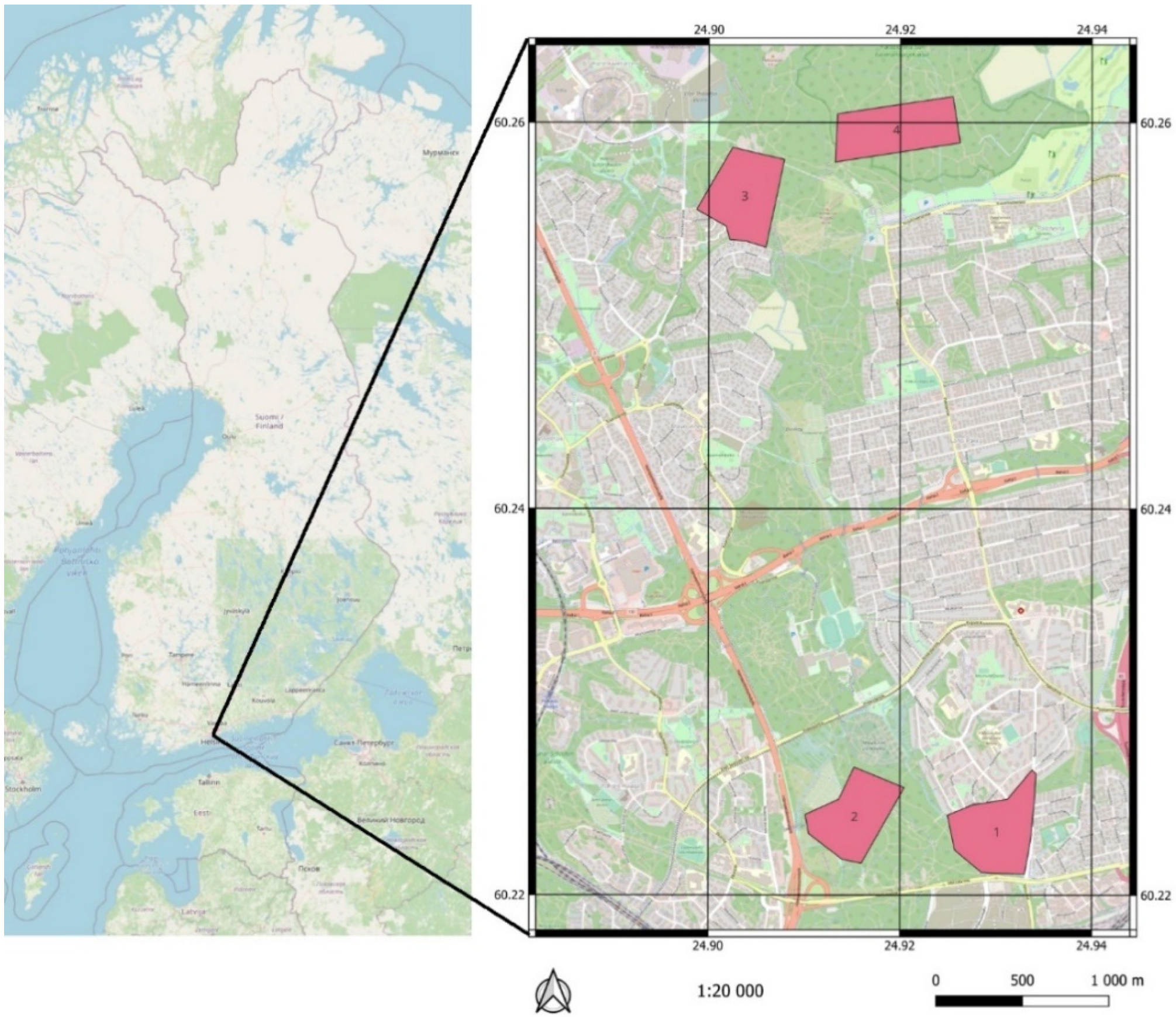
The objective of this study was to investigate the capabilities of UAV-based multispectral imagery in detecting declined trees at two different data collection times and compare the effect of phenology and data acquisition timing on the classification accuracy of declined trees. The tree decline was mainly caused by an ongoing bark beetle infestation. We hypothesized that the data acquisition timing, phenology, and life cycle stages of the bark beetle affect the detection accuracy of declined trees. To test this hypothesis, we collected field and UAV-based data in four forest areas on two occasions in May and September 2020. We also investigated the transferability of tree decline detection classifiers between the study areas. Transferable classifiers would greatly reduce the costs of tree decline mapping by reducing the need for costly field work. Our overarching aim is to support the development of remote sensing applications for detecting declined trees and mapping of bark beetle infestation.

2. Materials and Methods

2.1. Study Area

The study areas, which consisted of four approximately 20 ha forest areas, were in the Helsinki city central park area in Southern Finland (Figure 1). The forests were dominated by mature Norway spruce (Picea abies H. Karst.) with admixtures of Scots pine (Pinus sylvestris L.), Silver birch (Betula pendula Roth), European aspen (Populus tremula L.), rowan (Sorbus aucuparia L.) and common juniper (Juniperus communis L.). The forest areas had an ongoing infestation by I. typographus, which had started in 2017, and all the areas had existing groups of dead trees before the study was conducted during 2020.

2.2. UAV Data Collection

Drone flights were carried out on 20 and 22 May (4 flights) and on 11 and 14 September (5 flights) in the four test areas by the Finnish Geospatial Research Institute (FGI). Each of the areas were captured with RGB and multispectral cameras (Table 1). The Paloheinä East datasets (Area 4) were collected using FGI’s custom build drone that was equipped with Sony A7R digital camera with a Sony FE 35 mm f/2.8 ZA Carl Zeiss Sonnar T* lens, Micasense Altum Multispectral camera and Applanix APX-20 UAV GNSS and IMU system. The other areas were collected using Phantom 4 Pro V2.0 drone equipped with Micasense RedEdge M Multispectral camera. The ground sampling distances (GSD) were approximately 5 cm and 8 cm for Altum and RedEdge, respectively. The RedEdge and Altum have five cameras capturing blue (central wavelength: 475 nm; bandwidth: 32 nm), green (560 nm; 27 nm), red (668 nm; 14 nm), red edge (717 nm; 12 nm) and near-infrared (NIR) (842 nm; 57 nm) spectral bands.
Forward and side overlaps were approximately 80% and 80% for both multispectral cameras. Those overlaps resulted in photogrammetric blocks that ensured the area of interest was captured in more than nine overlapping images. All the areas included five ground control points (GCPs) that were measured with RTK GNSS receiver.

2.3. Multispectral Imagery Processing

The collected multispectral imagery was calibrated and processed using the Metashape Professional software package into orthorectified reflectance factor mosaics. The radiometric processing of the Micasense dataset was performed in Metashape as recommended by Micasense (2020a). Micasense data was loaded into Metashape as a multispectral camera, where the metadata of the images holding information about camera GPS data, calibration parameters, and radiometric parameters is recognized by the software. For the reflectance transformation, images of the camera’s reflectance panel taken before and after the flight were automatically located and identified by Metashape. In the orientation processing, full resolution images were used, number of the key points per image were 40,000, for tie points per image were 4000 and self-calibration options were used. Additionally, to speed up the orientation processing, preselection of image pairs was performed using downscaled images and their location information. The GCPs were measured on the images manually. Automatic outlier removal was performed on the basis of the residuals, as well as standard deviations of the tie point 3D coordinates and some outlier points were removed manually from the point cloud. After that, all interior (IOP) and exterior orientation parameters (EOP) and sparse point clouds were optimized. Next, dense point cloud calculation was carried out using full-resolution images and the mild point filtering feature and a further digital elevation model was calculated from that dense point cloud. Finally, orthomosaics were calculated with a GSD of 4.5 cm for the Altum imagery (Area 4) and 8.4 cm for the RedEdge-MX imagery (Areas 1–3) using the orthomosaic blending mode (Figure 2).

2.4. Tree Segmentation

The study areas were measured using airborne laser scanning (ALS) on 31 May 2015 by the city of Helsinki. This openly available data was used for tree segmentation, because of the better penetration capability of the laser pulses. The forests are not managed, thus, there were no forest operations between the ALS and UAV data collections. A digital terrain model (DTM) was developed based on ground points using a k-nearest neighbor approach (k = 10) with an inverse-distance weighting. The power for inverse-distance weighting was set to two. Then, the point cloud was height normalized by subtracting the ground height from each point above ground.
A pit-free canopy height model (CHM) at 50 cm resolution was produced using the height normalized point cloud and the CHM was smoothed using a focal mean filter with a 3 × 3 window [33]. Tree canopies were detected from the CHM using a local maximum filter with a minimum tree height of 3 m and a circular window with a diameter of 4 m. Individual trees were segmented using the CHM and the detected tree canopies using an algorithm developed by Dalponte and Coomes [34]. All the processing of the ALS data was conducted using the LidR package within the R software package [35,36]. To account for the difference between the timing of the tree segmentation and multispectral imagery, missing trees were visually identified from the orthomosaics and removed.

2.5. Reference Tree Data Collection and Tree Vitality Classification

The reference tree data was collected for training remote sensing classifiers, first from 18 May 2020 to 25 May 2020 and again from 11 September 2020 to 17 September 2020 in all the study areas (Table 1). In total, 466 reference trees were assessed in May and 556 in September. The trees were randomly selected based on the canopy condition aiming at a normal distribution of different tree vitality statuses. However, this was found to be challenging due to the lack of declined trees in some areas. The assessment focused on living mature Norway spruces that were in the upper canopy layer (i.e., dominant trees). Existing orthoimagery from the city of Helsinki was utilized in the field to locate individual trees and the vitality of Norway spruces was assessed by an expert based on the condition of the crown and the stem. The canopy was assessed based on the color of foliage into six different classes (points 0–5): healthy green, slightly faded green, yellowish, yellow, reddish/brown and grey. We also assessed defoliation into five classes (points 0–4): 0–10%, 10–25%, 25–50%, 50–75% and 75–100%, and the size of the canopy was examined. A significantly smaller canopy vertical size was considered as an indication of decline (points 0–1). Points were given based on the condition so that a zero was given for the healthiest class and one point for each class towards more severe symptoms. Stems were also assessed for recent thin flows of resin (indicating a bark beetle infestation) and bark structural damage into three classes (points 0–2): not detected, moderate damage and severe damage.
A health classification of the reference trees was conducted based on the symptoms assessed in the field by multiplying the points of canopy symptoms discoloration and defoliation with 1.5 and summing all the points together for each tree (Table 2). The canopy symptoms were weighted, because they are easier to detect from an aerial point of view. Every tree that had a point rating of two or under was classified as a healthy tree and every tree with more than two points was classified as a declined tree. In addition to healthy and declined trees, dead trees (n = 203) were located and classified visually from the RGB orthoimagery that was collected for the study. The trees having reddish, brown or grey crowns were considered as dead trees.

2.6. Multispectral Imagery Features

A set of statistical features were calculated for each tree using the calibrated multispectral reflectance factor orthomosaics, which are referred to as spectral features in this paper. To avoid the influence of shadows on the features, pixels that had a sum of reflectance factor values of all bands of less than 0.1 were excluded from the analysis [25]. This threshold was visually identified to reduce the number of shadows. The features (Table 3), that describe the reflectance distribution, were calculated for the tree segments for each band and for each normalized difference index (NDI) that were calculated for each pixel using the following equation:
NDI1,2 = (ρ1 − ρ2)/(ρ1 + ρ2)
where ρ is the wavelength. The NDI was calculated using different combinations of wavelengths: NIR + red, red-edge + red, red + blue, red + green and NIR + red-edge. The different NDI spectral features were calculated due to their ability to reduce the effect of bidirectional reflectance distribution function on the measured values, which are challenging to account for in reflectance calibration [37]. Additionally, the changes in tree canopy reflectance spectrum can be assumed to affect the ratios between different bands [25].

2.7. Statistical Analysis

We used a t-test to investigate the difference in spectral reflectance factors between tree vitality classes: healthy, declined and dead. p-value was used as a measure of significance in difference. The t-test was also used to assess differences in spectral reflectance factors of each tree vitality class between different areas. We used the mean value per tree segment of each band and each calculated NDI to perform this assessment.
We used a machine learning algorithm, Random Forest, as a classification method for classifying the different vitality classes due to its ability to handle high data dimensionality and multicollinearity [38,39]. Vitality classification was conducted independently for the May and September data. The datasets were randomly divided into a training set (75%) and an independent test set (25%) using stratified sampling of each tree vitality class to calculate the accuracy of the developed models. Model parameters were 1000 “decision trees” (influences the stability of the model) and the maximum number of features was 19, which is the square root of the total number of features [40]. Data division and Random Forest classification was performed 30 times to assess the variation in the accuracy of the models. The range of classification accuracies achieved is reported using the overall classification accuracy, map-level image classification efficacy (MICE) and classification accuracy of each tree vitality class [41]. MICE outputs a value that ranges between 0 and 1, where a zero value indicates an output as good as random classification and value of 1 indicates perfect classification. Variable importance was calculated for each Random Forest model using mean decrease accuracy (MEA) and the mean of the MEA of all the 30 model runs was calculated and reported.
Random Forest classifiers were also trained using each of the areas as a training dataset and the other areas as test datasets to investigate the transferability of the developed classifiers. In addition, a similar investigation was conducted for the areas that were found to have the most similar spectral reflectance factors based on the conducted t-tests. Overall workflow is presented in Figure 3.

3. Results

3.1. Spectral Reflectance Factors of Different Vitality Classes

Average spectral reflectance factors of the different tree vitality classes showed significant differences (p < 0.05) in both spring and fall datasets (Figure 4). The largest differences in reflectance factors between the vitality classes were found in the blue and red bands. Dead trees showed increased reflectance factors in the blue and red bands, but a decreased reflectance factors in the red-edge and NIR bands in comparison to the healthy and declined trees. The difference in reflectance factor between healthy and declined trees was greater in the fall dataset. Declined trees there showed a significant increase in reflectance factors in all bands except for the NIR band. In the spring dataset, the red-edge and NIR bands did not show a significant difference.
Considering reflectance factors of different areas (Appendix A), in the spring datasets, the Area 3 had the lowest values and in the autumn datasets the Areas 1–2 had the lowest values. These differences were most likely due to the non-optimal radiometric correction. In Area 4, band 5 was brighter, relative to the other bands, than in the other areas. One possible explanation for this could be that the datasets in Area 4 were collected using the Micasense Altum while the other areas were collected using the Micasene RedEdge M. In the spring dataset, in Area 4 the declined class appeared to have lower reflectance factors than the healthy class, which is opposite to all other datasets. We could not find any explanation for this behavior.
The results revealed differences in the similarity of spectral reflectance factors between different areas (Figure 5). The areas that were closer to each other showed better similarity in the spectral reflectance factors. The t-tests showed that Areas 1 and 2 had on average smaller differences in spectral reflectance factors than each of Areas 3 and 4. Similarly, Areas 3 and 4 showed smaller differences in spectral reflectance factors between each other for the spring data, but not the fall data.
The similarity values between areas varied in spring and autumn. On average, greater similarity in spectral reflectance factors between areas was observed for the fall data than the spring data. However, the spectral reflectance factors were more similar between Areas 3 and 4 for the spring data.

3.2. The Prediction of Tree Vitality Classes

The repeated Random Forest model runs with all the areas pooled and with each area separately revealed some variation in model accuracy (Table 4). The overall accuracy of the tree vitality predictions varied between 73.9% and 89.1% for the spring dataset and between 83.5% and 87.2% for the fall dataset. The MICE values varied between 0.58 and 0.82 for the spring dataset and between 0.72 and 0.78 for the fall dataset.
Class accuracies showed variation between classes (Table 5). The highest prediction accuracies were achieved for the dead trees with a mean of 95.7% and 98.7% for spring and fall datasets, respectively. Healthy trees were identified with a mean accuracy of 80.4% and 82.8% for the spring and fall datasets, respectively. Declined trees showed the lowest detection accuracies, with mean accuracies of 54.2% and 64.4% for the spring and fall datasets, respectively. The poorest results were obtained for the declined class in the Fall_2 datasets that had a remarkably low number of reference trees. The predicted tree vitality maps for each area and each dataset can be observed in the Appendix A.

3.3. Transferability of the Random Forest Classifiers between Areas

We tested how the tree vitality classification models are transferable between different areas using a single area as training data and predicting the tree vitality classes for other areas. The overall accuracies of the predictions (Table 6) were lower than when all the areas used in the prediction models, ranging between 59.3% and 80.1%. However, larger differences were found in the class accuracies (Table 7). Generally, the dead trees were accurately classified with class accuracies above 92% for all models, but healthy and declined trees showed high variability in their class accuracies depending on the area that was used for training the model. Most of the trained RF models classified healthy trees with decent accuracies, but very low classification accuracies were achieved when Area 4 was used for training the model. Generally, the classification accuracy of healthy and declined trees was not stable with few exceptions. The fall dataset of area 3 and spring dataset of area 1 resulted in a more balanced classification accuracy of healthy and declined trees, but fewer than 68% of the trees were correctly classified. The healthy, declined and dead class accuracies were for the spring dataset 93.1%, 18.0% and 95.0%, respectively, and for the fall dataset 65.1%, 63.7%, and 98.8%, respectively. More accurate results were achieved when using those areas for training and testing that were identified as similar in the analysis of spectral similarity in Section 3.1. In these comparisons the overall accuracies were 68.5–83.7%. The classification accuracies for the cases with the highest overall accuracies were 95.1, 45.5 and 96.2%, for the healthy, declined and dead classes, respectively, in spring and 71.0, 78.6, 99%, respectively, in fall.

3.4. Variable Importance in Tree Vitality Class Predictions

The most important variables in predicting tree vitality class were in NDI spectral features (Table 8). NDIedge-red spectral features showed the highest importance for both spring and fall datasets. The most important features also included spectral features from NDIred-NIR and NDIred-green.

4. Discussion

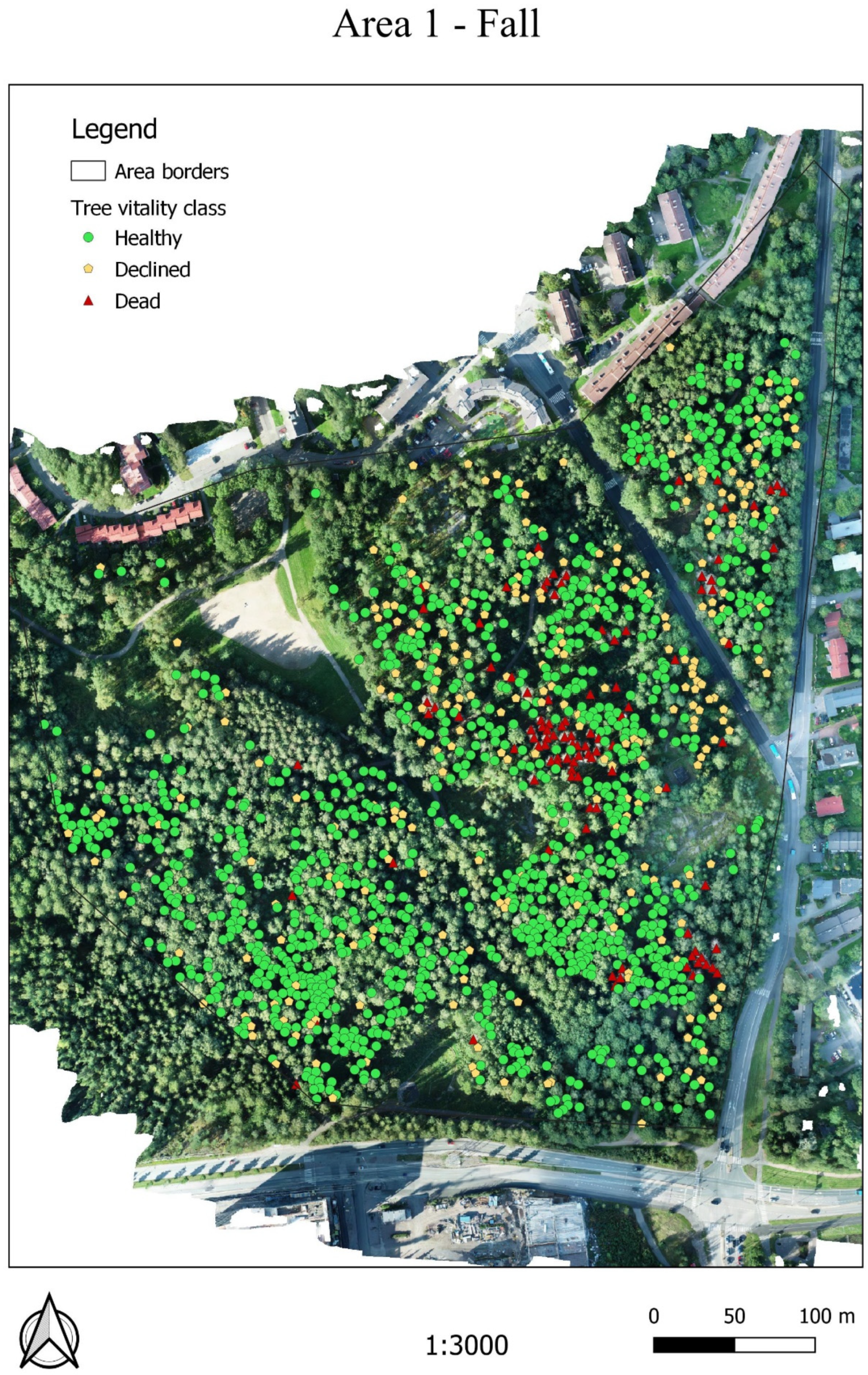
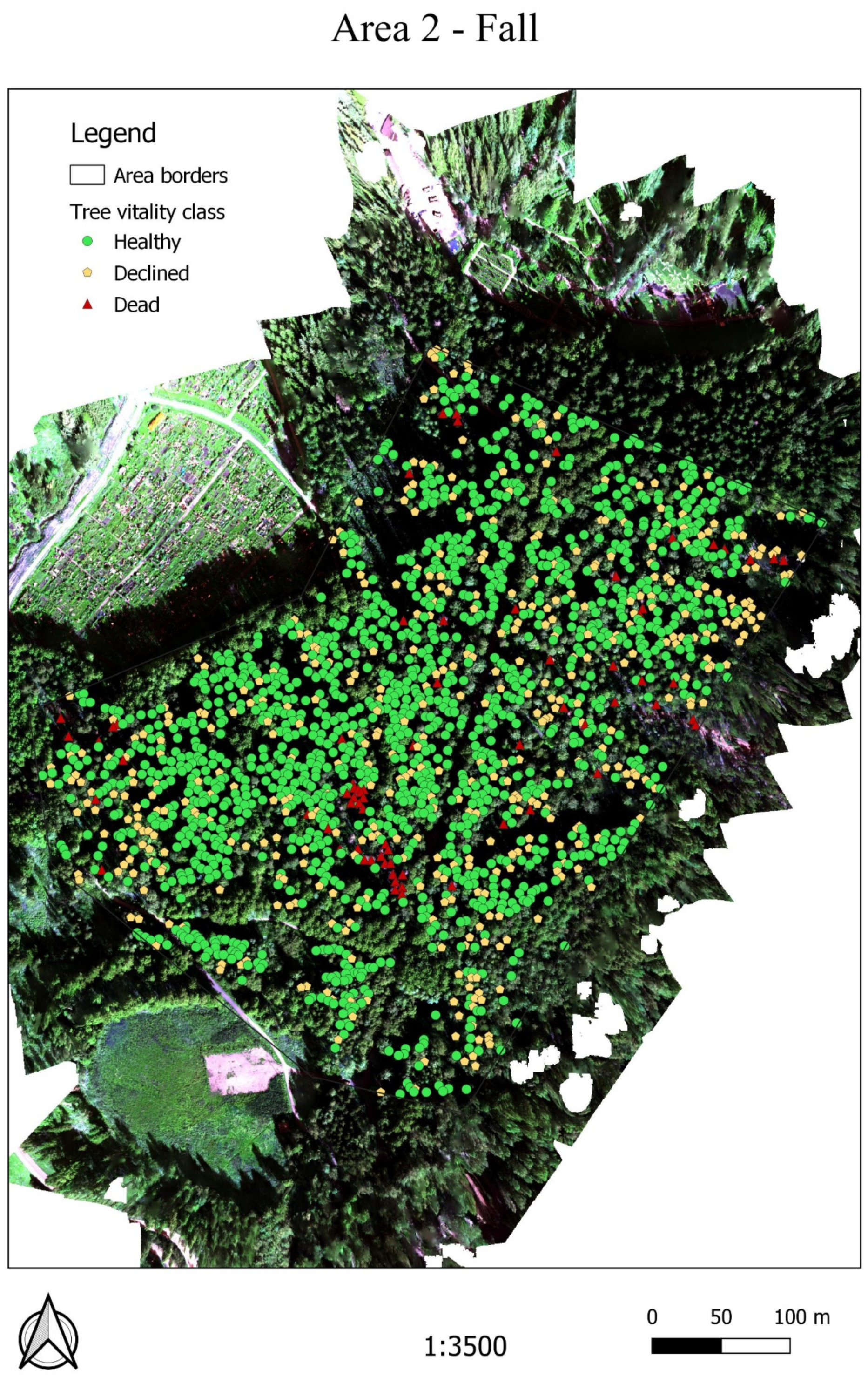
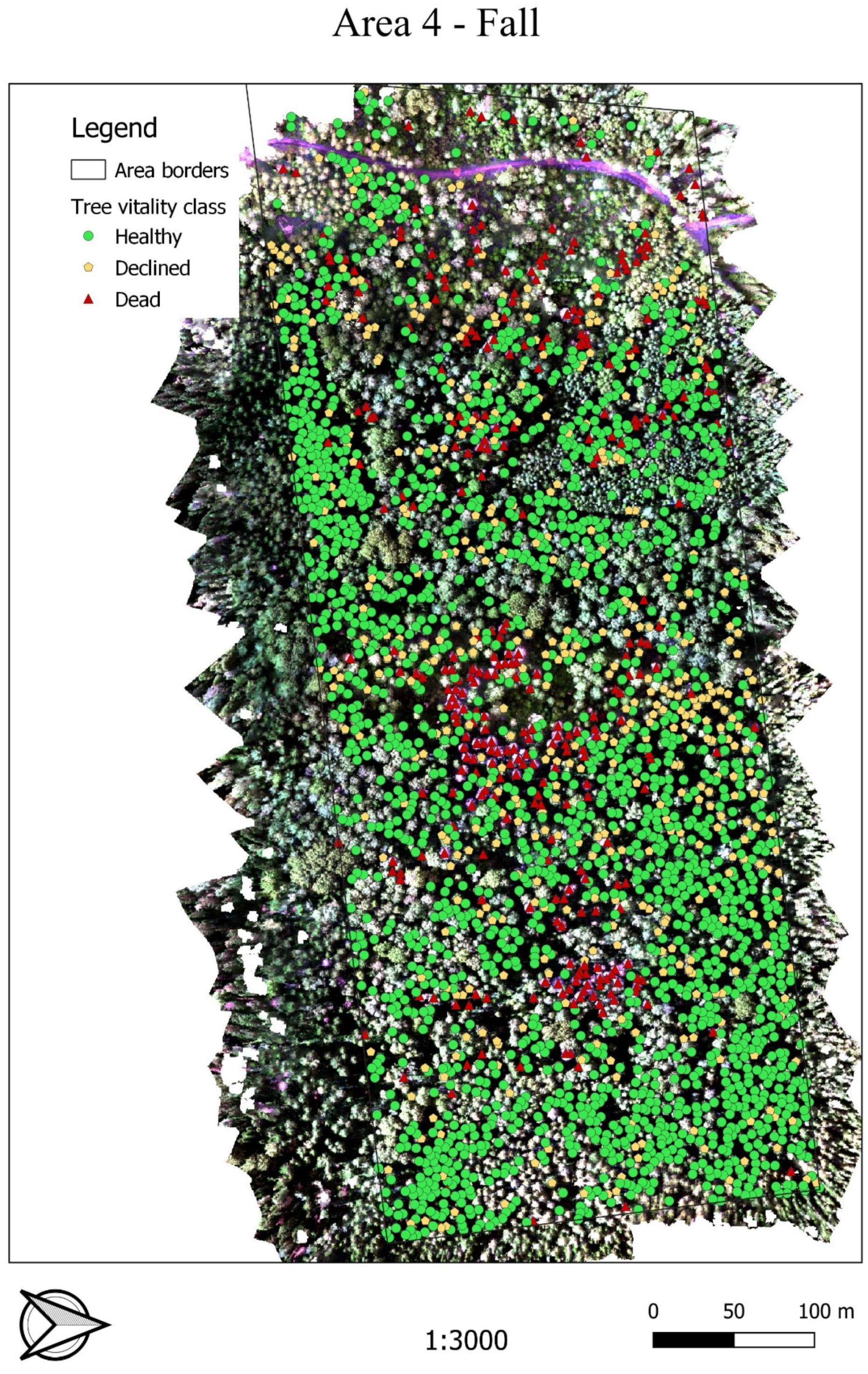
The aim of this study was to investigate the capabilities of UAV-based multispectral imagery in detecting declined trees at two different data collection times when bark beetle infestation had separate active statuses based on a life cycle of the species. Further, we aimed to compare the effect of data acquisition timing on the detection accuracy of declined trees. We hypothesized that the data acquisition timing and tree phenology affect the detection accuracy of declined trees. We also investigated the transferability of the trained Random Forest models in the detection of tree decline classes between the four study areas. To test how data acquisition timing and phenology affects the detection accuracy of declined trees, we developed a Random Forest based classification approach for classifying Norway spruces into various health classes, including healthy, declined and dead. The average overall accuracy and MICE value were 78.2% and 0.66, respectively, in spring and 84.5% and 0.76, respectively, in fall. When considering all the study areas, the mean accuracies of the healthy, declined and dead classes were 80.4%, 54,2% and 95.7%, respectively, for the spring dataset, and 82.8%, 64.4% and 98.7%, respectively, for the fall dataset. Considering the area-specific results, the best results were 91.4%, 58.7% and 100%, respectively, in Area 1 in spring, and 88.5%, 65.4% and 99.2%, respectively, in Area 4 in fall. Based on our results, it seems that data acquired during fall or the end of summer before winter dormancy provides more accurate tree vitality classification compared to data acquired during the spring.
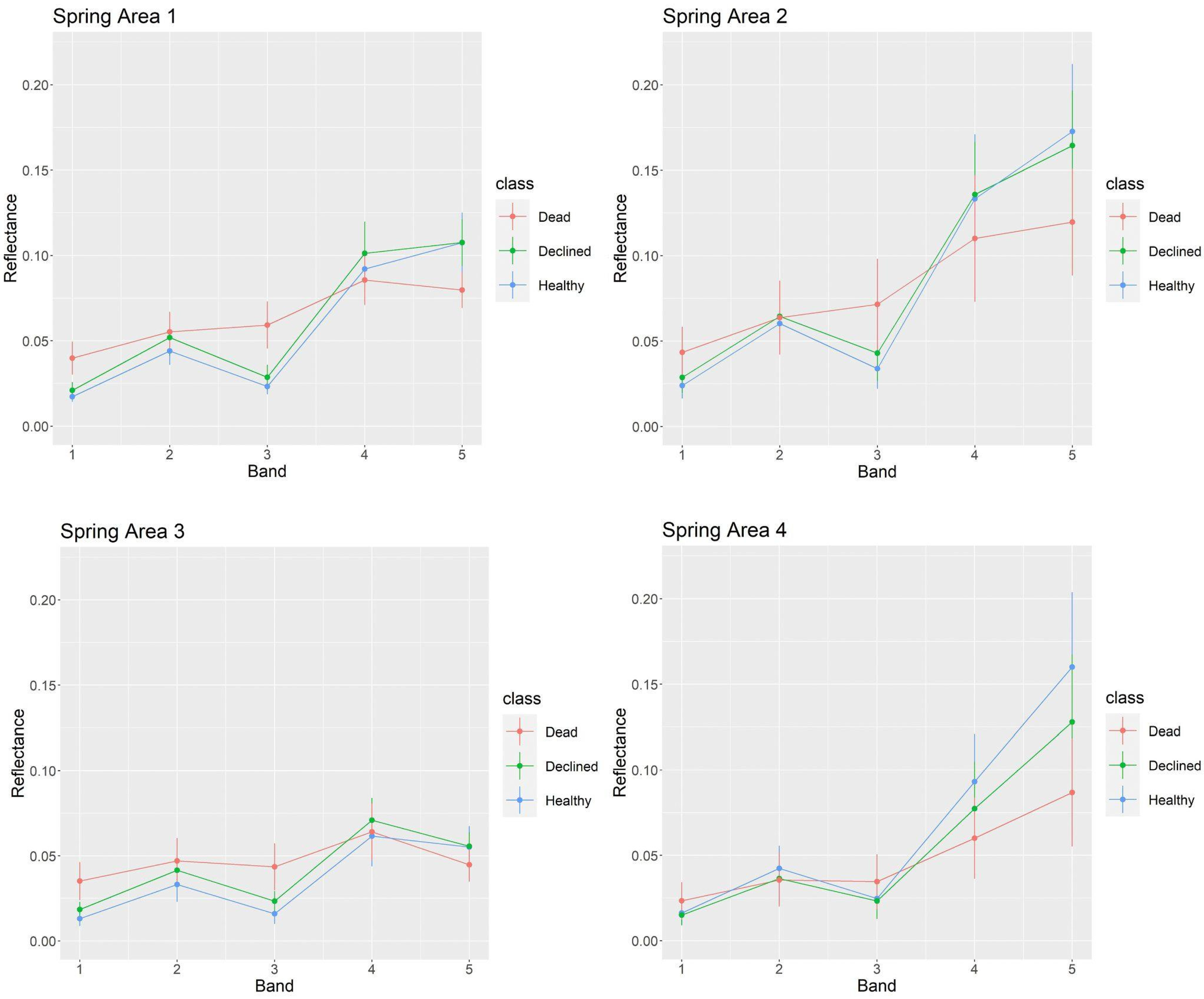
There were differences between spring and fall reflectance factors, which were at least partially due to the non-optimal radiometric correction. In Area 4, band 5 was brighter in relation to the other bands than in the other areas. One possible explanation for this could be that in datasets in Area 4 were collected using the Micasense Altum while the other areas were collected using the Micasene RedEdge M. In the spring dataset, Area 4 the declined class appeared to have lower reflectance factors than the healthy class, which is opposite to all other datasets. We could not find any explanation for this behavior. The differences in reflectance factors are also a likely explanation to the high importance of NDI type reflectance features in classifying tree vitality classes, because vegetation indices are able to partly reduce the effect of varying illumination conditions. The NDIedge-red spectral features showed the highest importance in classifying tree vitality in both spring and fall datasets; thus, the feature selection was similar between the data acquisition timings.
The results of this study were in line with previous studies that used UAV-imagery for monitoring of tree vitality conditions. For example, Näsi et al. [25] obtained with the SVM classifier using hyperspectral images, collected in August, showing producer’s accuracies of 89%, 47% and 58%, for healthy, infested and dead classes, respectively. When using the independent test dataset, the leave-one-out producer’s accuracies were 86%, 67% and 81%, respectively. The results of this study are also in line with the study of Kloucek et al. [27] where the best results were obtained in the end of the infestation period (overall accuracy: 96%) 78%–96% with a Maximum Likelihood classifier with less than 55 reference trees. In the study of Honkavaara et al. [42], there was not such a high difference in classification accuracies between different dates. The comparison to this study is not as straightforward since the time span was shorter (August–October), when all trees stayed in the green-attack phase during the data collection period, indicating a low colonization rate. Further, many trees in the area were suffering from root rot. Potential explanations for the better accuracies in the present study were the larger number of reference trees that managed to explain the data more comprehensively as well as the potentially better performance of the Random Forest classifier than SVM or Maximum Likelihood classifiers.
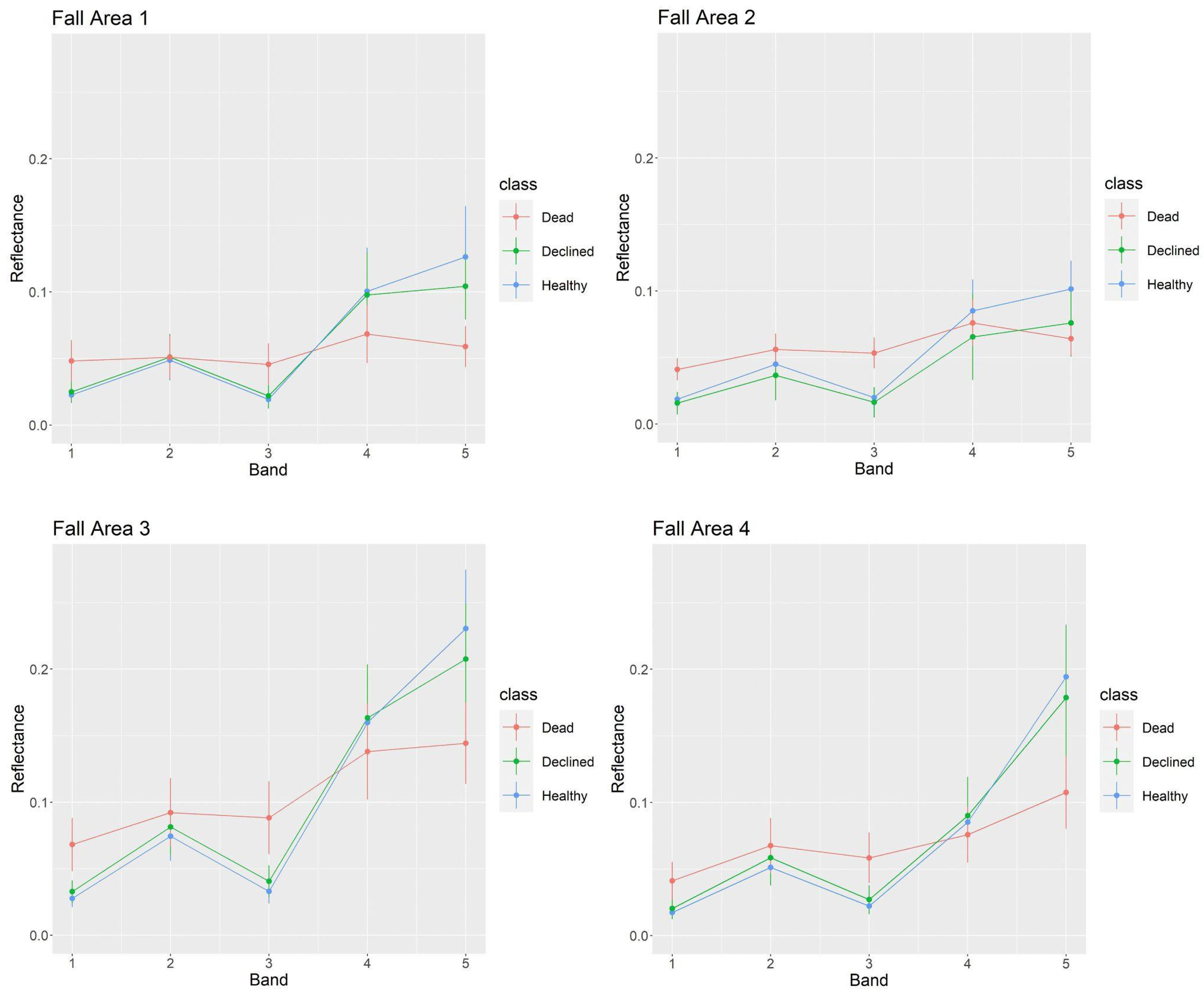
Considering the data collection timing and phenology aspects, it appeared that the fall dataset provided better results than the spring dataset. For example, the overall accuracy for the combined classifier was 78.2% in spring and 84.5% in fall and the corresponding averages for the area-specific classifiers were 79.4% and 85.7%. Similar conclusions could be obtained from the analysis of the health classification results. The better results in fall could be explained by the smaller deviation in the autumn dataset as the spectral response of the new growth approaches the response of the growth in earlier years, whereas in spring the varying amount of bright green colour causes variability for the spectral values. The growth of needles and leaves was only starting in the spring dataset, thus, there may be considerable variation in the spring phenology of individual trees due to differences in microclimate, soil temperature and aspect in relation to the sun, which could cause increased variation in spectral responses.
The illumination conditions influence the reflectance factors due to the anisotropic behaviour of the canopy reflectance. The solar elevation was 35.7–49.3° in the spring dataset and 23.2–31.9° in the fall dataset, the larger variation in the spring dataset might have contributed to the larger reflectance factor differences in comparison to the fall dataset. Furthermore, the illumination conditions varied between mostly cloudy and completely sunny, which could also have an impact. For example, the large solar elevation differences of 24.9°–31.44° and variation from mostly cloudy to sunny conditions might have caused the great differences in the comparison for fall datasets of Area 3 and 4. The best similarities were obtained between Area 1 and 2, which were captured in sunny conditions within two hours in spring as well as in mostly sunny conditions and only with approx. 5° solar elevation difference in fall.
We also investigated the transferability of the developed RF-model in classifying tree decline classes. The best overall accuracies of the transformed models were 74.5% and 78.7%, and the best MICE values were 0.61 and 0.67, respectively, for the spring and autumn, and these were obtained using the Area 3 data to train the classifier, which might be due to forest structural and spectral similarity to other areas. When training and testing with the datasets observed to be statistically similar, the results improved, providing the best overall accuracy of 81.6% and 83.7% and MICE values of 0.73 and 0.75, respectively to the spring and fall datasets. Although the results seem promising, they were not stable and further improvements in the methodology are needed to make this approach more reliable. Particularly, there appeared quite large differences in reflectance values in different datasets, which were likely to be at least partially due to the non-modelled factors in the radiometric processing of the standard radiometric processing chain that was used in this study. The recent review by Aasen et al. [43] suggested various techniques for radiometric processing. The state-of-the-art techniques provide tools for atmospheric correction [44,45]. However, the methods for accounting for the reflectance anisotropy are still missing from most of the presented processing chains; one of the existing solutions is the radiometric block adjustment presented by Honkavaara et al. [46]. By solving the deviations caused by the illumination, the amount of reference data for the classifiers could be decreased and this way better efficiency could be obtained for the tree vitality mapping processes. It is also interesting to notice that there were not great differences between the results of the combined classifier or the average/median values from the separate area classifiers. This indicates that the Random Forest could explain differences due to solar elevations and illumination conditions. However, in further studies also the novel algorithms such as convolutional neural networks and the deep learning techniques will be of interest. For example Safonova et al. [32] obtained promising results by using a RGB camera for classifying tree decline classes caused by a bark beetle (P. proximus) in fir forest.
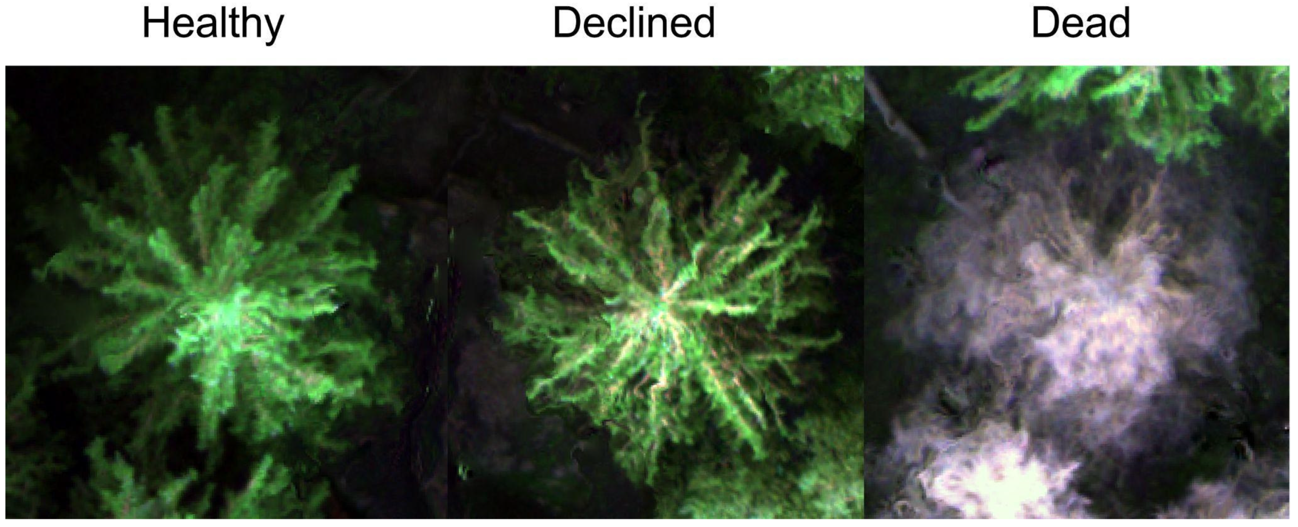
We assigned various trees having symptoms to the “declined” class, thus we did not separate the spruces in the “green-attack” phase and the more yellowish phases. We will continue the analysis to evaluate if the “green-attacked” trees could be separated from the other phases, which would enable the efficient management of the bark beetle infestation, e.g., by enabling sanitation cutting of colonized trees before the swarming of the following generation. Particularly the novel narrow-band hyperspectral sensors suitable for UAVs are highly promising tools for identifying small changes in tree vitality even before they can be observed via visual assessment of the crown as stated Einzmann et al. [47] using hyperspectral needle reflectance measured in the ground and hyperspectral crown reflectance measured from aircraft. Utilizing the proposed approach, it will be possible to generate tree vitality maps cost efficiently from forest areas. By optimizing the timing of data collection, one can improve tree decline classification accuracy, and transferable machine learning models increase the cost-efficiency of UAV-based tree decline monitoring. The information on tree decline is also relevant for developing risk models to estimate potential forthcoming disturbance and knowledge considering the distribution spread of the bark beetle infestation in forests. The frequent maps will provide information for decision makers and forest managers to support their forest management towards climate and pest insect resilient forests.

5. Conclusions

The use of UAV-multispectral data for classifying tree vitality to dead, attacked, and healthy classes was explored using data collected in spring and fall to investigate the effect of acquisition timing on classification results. We found that data acquisition in the fall (early September in this case) resulted in more accurate tree vitality classification indicating that multispectral image data has more value for tree vitality mapping in the end of the growing season. We conclude that multispectral UAV-based imagery provides benefits for mapping spruce tree decline when acquired close to end of season compared to imagery acquired during spring.
Moreover, the transferability of the trained RF-models was investigated by applying the trained models to a sub-study area to others and vice versa. When we tested the transferability of tree decline detection classifiers between the study areas, the obtained classification accuracies decreased only slightly. However, the obtained classifications were not stable and further improvements in the methodology are needed to make transferability more reliable.

Author Contributions

Conceptualization, S.J. and J.R.; methodology, S.J., R.N. and N.K.; validation, S.J. and N.K.; formal analysis, S.J. and E.H.; investigation, S.J. and R.N.; resources, J.R., E.H. and M.H.; data curation, S.J. and N.K.; visualization, M.I.; writing—original draft preparation, S.J., R.N. and E.H.; writing—review and editing, M.I., N.S., P.L.-S., J.R., J.H., M.H., M.V. and H.H.; supervision, M.V.; funding acquisition, S.J., E.H., M.V., M.H. and J.H. All authors have read and agreed to the published version of the manuscript.

Funding

The research was funded by the Academy of Finland under grants 330422, 327861, 315079, 345166, 348643, 346383, 337810, by the Ministry of Agriculture and Forestry of Finland (project Monituho, decision number VN/5514/2020) and by the Doctoral Program in Sustainable Use of Renewable Natural Resources (AGFOREE) at the University of Helsinki. This study has been performed with affiliation to the Academy of Finland Flagship Forest–Human–Machine Interplay—Building Resilience, Redefining Value Networks and Enabling Meaningful Experiences (UNITE) (decision no 337127).

Institutional Review Board Statement

Not applicable.

Informed Consent Statement

Not applicable.

Data Availability Statement

Data is available upon request from the corresponding author and will be made available from a public repository during 2022.

Acknowledgments

We are thankful to the City of Helsinki for their co-operation and especially to Vesa Koskikallio for all the help. We would also like to thank the anonymous reviewers for their comments.

Conflicts of Interest

The authors declare no conflict of interest. The funders had no role in the design of the study; in the collection, analyses, or interpretation of data; in the writing of the manuscript, or in the decision to publish the results.

Appendix A

The appendix contains figures of spectral reflectance factors of each tree vitality class for each area and each data collection (spring: Figure A1, fall: Figure A2) and maps of classified tree vitality (healthy, declined and dead) for each area and each data collection (Figure A3, Figure A4, Figure A5, Figure A6, Figure A7, Figure A8, Figure A9 and Figure A10).
Figure A1. The mean and standard deviation (error bars) of spectral reflectance for each band and tree vitality class for each area in the spring dataset.
Remotesensing 14 00909 g0a1
Figure A2. The mean and standard deviation (error bars) of spectral reflectance for each band and tree vitality class for each area in the fall dataset.
Remotesensing 14 00909 g0a2
Figure A3. Tree vitality classification to healthy, declined and dead classes for the spring data collection for Area 1 with RGB orthomosaic of the fall dataset in the background.
Remotesensing 14 00909 g0a3
Figure A4. Tree vitality classification to healthy, declined and dead classes for the fall data collection for Area 1 with RGB orthomosaic of the fall dataset in the background.
Remotesensing 14 00909 g0a4
Figure A5. Tree vitality classification to healthy, declined and dead classes for the spring data collection for Area 2 with RGB orthomosaic of the fall dataset in the background.
Remotesensing 14 00909 g0a5
Figure A6. Tree vitality classification to healthy, declined and dead classes for the fall data collection for Area 2 with RGB orthomosaic of the fall dataset in the background.
Remotesensing 14 00909 g0a6
Figure A7. Tree vitality classification to healthy, declined and dead classes for the spring data collection for Area 3 with RGB orthomosaic of the fall dataset in the background.
Remotesensing 14 00909 g0a7
Figure A8. Tree vitality classification to healthy, declined and dead classes for the fall data collection for Area 3 with RGB orthomosaic of the fall dataset in the background.
Remotesensing 14 00909 g0a8
Figure A9. Tree vitality classification to healthy, declined and dead classes for the spring data collection for Area 4 with RGB orthomosaic of the fall dataset in the background.
Remotesensing 14 00909 g0a9
Figure A10. Tree vitality classification to healthy, declined and dead classes for the fall data collection for Area 4 with RGB orthomosaic of the fall dataset in the background.
Remotesensing 14 00909 g0a10

References

  1. Shashkov, M.; Ivanova, N.; Shanin, V.; Grabarnik, P. Ground Surveys Versus UAV Photography: The Comparison of Two Tree Crown Mapping Techniques. In Proceedings of the Information Technologies in the Research of Biodiversity, Irkutsk, Russia, 11–14 September 2018; Bychkov, I., Voronin, V., Eds.; Springer International Publishing: Cham, Switzerland, 2019; pp. 48–56. [Google Scholar] [CrossRef]
  2. Getzin, S.; Nuske, R.S.; Wiegand, K. Using Unmanned Aerial Vehicles (UAV) to Quantify Spatial Gap Patterns in Forests. Remote Sens. 2014, 6, 6988–7004. [Google Scholar] [CrossRef] [Green Version]
  3. Getzin, S.; Wiegand, K.; Schöning, I. Assessing biodiversity in forests using very high-resolution images and unmanned aerial vehicles. Methods Ecol. Evol. 2011, 3, 397–404. [Google Scholar] [CrossRef]
  4. Chianucci, F.; Disperati, L.; Guzzi, D.; Bianchini, D.; Nardino, V.; Lastri, C.; Rindinella, A.; Corona, P. Estimation of canopy attributes in beech forests using true colour digital images from a small fixed-wing UAV. Int. J. Appl. Earth Obs. Geoinf. 2016, 47, 60–68. [Google Scholar] [CrossRef] [Green Version]
  5. Puliti, S.; Ørka, H.O.; Gobakken, T.; Næsset, E. Inventory of Small Forest Areas Using an Unmanned Aerial System. Remote Sens. 2015, 7, 9632–9654. [Google Scholar] [CrossRef] [Green Version]
  6. Giannetti, F.; Chirici, G.; Gobakken, T.; Næsset, E.; Travaglini, D.; Puliti, S. A new approach with DTM-independent metrics for forest growing stock prediction using UAV photogrammetric data. Remote Sens. Environ. 2018, 213, 195–205. [Google Scholar] [CrossRef]
  7. Michez, A.; Piégay, H.; Lisein, J.; Claessens, H.; Lejeune, P. Classification of riparian forest species and health condition using multi-temporal and hyperspatial imagery from unmanned aerial system. Environ. Monit. Assess. 2016, 188, 146. [Google Scholar] [CrossRef] [Green Version]
  8. Gini, R.; Passoni, D.; Pinto, L.; Sona, G. Use of Unmanned Aerial Systems for multispectral survey and tree classification: A test in a park area of northern Italy. Eur. J. Remote Sens. 2014, 47, 251–269. [Google Scholar] [CrossRef]
  9. Saarinen, N.; Vastaranta, M.; Näsi, R.; Rosnell, T.; Hakala, T.; Honkavaara, E.; Wulder, M.A.; Luoma, V.; Tommaselli, A.M.G.; Imai, N.N.; et al. Assessing Biodiversity in Boreal Forests with UAV-Based Photogrammetric Point Clouds and Hyperspectral Imaging. Remote Sens. 2018, 10, 338. [Google Scholar] [CrossRef] [Green Version]
  10. Feduck, C.; McDermid, G.J.; Castilla, G. Detection of Coniferous Seedlings in UAV Imagery. Forests 2018, 9, 432. [Google Scholar] [CrossRef] [Green Version]
  11. Puliti, S.; Solberg, S.; Granhus, A. Use of UAV Photogrammetric Data for Estimation of Biophysical Properties in Forest Stands Under Regeneration. Remote Sens. 2019, 11, 233. [Google Scholar] [CrossRef] [Green Version]
  12. Imangholiloo, M.; Saarinen, N.; Markelin, L.; Rosnell, T.; Näsi, R.; Hakala, T.; Honkavaara, E.; Holopainen, M.; Hyyppä, J.; Vastaranta, M. Characterizing Seedling Stands Using Leaf-Off and Leaf-On Photogrammetric Point Clouds and Hyperspectral Imagery Acquired from Unmanned Aerial Vehicle. Forests 2019, 10, 415. [Google Scholar] [CrossRef] [Green Version]
  13. Yuan, C.; Zhang, Y.; Liu, Z. A survey on technologies for automatic forest fire monitoring, detection, and fighting using unmanned aerial vehicles and remote sensing techniques. Can. J. For. Res. 2015, 45, 783–792. [Google Scholar] [CrossRef]
  14. Kinaneva, D.; Hristov, G.; Raychev, J.; Zahariev, P. Early forest fire detection using drones and artificial intelligence. In Proceedings of the 2019 42nd International Convention on Information and Communication Technology, Electronics and Microelectronics (MIPRO), Opatija, Croatia, 20–24 May 2019; pp. 1060–1065. [Google Scholar]
  15. Lehmann, P.; Ammunét, T.; Barton, M.; Battisti, A.; Eigenbrode, S.D.; Jepsen, J.U.; Kalinkat, G.; Neuvonen, S.; Niemelä, P.; Terblanche, J.S.; et al. Complex responses of global insect pests to climate warming. Front. Ecol. Environ. 2020, 18, 141–150. [Google Scholar] [CrossRef] [Green Version]
  16. Biedermann, P.H.; Müller, J.; Grégoire, J.-C.; Gruppe, A.; Hagge, J.; Hammerbacher, A.; Hofstetter, R.W.; Kandasamy, D.; Kolarik, M.; Kostovcik, M.; et al. Bark Beetle Population Dynamics in the Anthropocene: Challenges and Solutions. Trends Ecol. Evol. 2019, 34, 914–924. [Google Scholar] [CrossRef] [PubMed] [Green Version]
  17. Seidl, R.; Rammer, W.; Jäger, D.; Lexer, M.J. Impact of bark beetle (Ips typographus L.) disturbance on timber production and carbon sequestration in different management strategies under climate change. For. Ecol. Manag. 2008, 256, 209–220. [Google Scholar] [CrossRef]
  18. Blomqvist, M.; Kosunen, M.; Starr, M.; Kantola, T.; Holopainen, M.; Lyytikäinen-Saarenmaa, P. Modelling the predisposition of Norway spruce to Ips typographus L. infestation by means of environmental factors in southern Finland. Forstwiss. Centralblatt 2018, 137, 675–691. [Google Scholar] [CrossRef]
  19. Jönsson, A.M.; Appelberg, G.; Harding, S.; Bärring, L. Spatio-temporal impact of climate change on the activity and voltinism of the spruce bark beetle, Ips typographus. Glob. Chang. Biol. 2009, 15, 486–499. [Google Scholar] [CrossRef]
  20. Hlásny, T.; Krokene, P.; Liebhold, A.; Montagné-Huck, C.; Müller, J.; Qin, H.; Raffa, K.; Schelhaas, M.; Seidl, R.; Svoboda, M. Living with Bark Beetles: Impacts, Outlook and Management Options; European Forest Institute: Joensuu, Finland, 2019. [Google Scholar]
  21. Junttila, S.; Holopainen, M.; Vastaranta, M.; Lyytikäinen-Saarenmaa, P.; Kaartinen, H.; Hyyppä, J.; Hyyppä, H. The potential of dual-wavelength terrestrial lidar in early detection of Ips typographus (L.) infestation—Leaf water content as a proxy. Remote Sens. Environ. 2019, 231, 111264. [Google Scholar] [CrossRef]
  22. Torresan, C.; Berton, A.; Carotenuto, F.; Di Gennaro, S.F.; Gioli, B.; Matese, A.; Miglietta, F.; Vagnoli, C.; Zaldei, A.; Wallace, L. Forestry applications of UAVs in Europe: A review. Int. J. Remote Sens. 2018, 38, 2427–2447. [Google Scholar] [CrossRef]
  23. Manfreda, S.; McCabe, M.F.; Miller, P.E.; Lucas, R.; Madrigal, V.P.; Mallinis, G.; Ben Dor, E.; Helman, D.; Estes, L.; Ciraolo, G.; et al. On the Use of Unmanned Aerial Systems for Environmental Monitoring. Remote Sens. 2018, 10, 641. [Google Scholar] [CrossRef] [Green Version]
  24. Lehmann, J.R.K.; Nieberding, F.; Prinz, T.; Knoth, C. Analysis of Unmanned Aerial System-Based CIR Images in Forestry—A New Perspective to Monitor Pest Infestation Levels. Forests 2015, 6, 594–612. [Google Scholar] [CrossRef] [Green Version]
  25. Näsi, R.; Honkavaara, E.; Blomqvist, M.; Lyytikäinen-Saarenmaa, P.; Hakala, T.; Viljanen, N.; Kantola, T.; Holopainen, M. Remote sensing of bark beetle damage in urban forests at individual tree level using a novel hyperspectral camera from UAV and aircraft. Urban For. Urban Green. 2018, 30, 72–83. [Google Scholar] [CrossRef]
  26. Toth, D.; Maitah, M.; Maitah, K.; Jarolínová, V. The Impacts of Calamity Logging on the Development of Spruce Wood Prices in Czech Forestry. Forests 2020, 11, 283. [Google Scholar] [CrossRef] [Green Version]
  27. Klouček, T.; Komárek, J.; Surový, P.; Hrach, K.; Janata, P.; Vašíček, B. The Use of UAV Mounted Sensors for Precise Detection of Bark Beetle Infestation. Remote Sens. 2019, 11, 1561. [Google Scholar] [CrossRef] [Green Version]
  28. Minařík, R.; Langhammer, J.; Lendzioch, T. Detection of Bark Beetle Disturbance at Tree Level Using UAS Multispectral Imagery and Deep Learning. Remote Sens. 2021, 13, 4768. [Google Scholar] [CrossRef]
  29. Minařík, R.; Langhammer, J.; Lendzioch, T. Automatic Tree Crown Extraction from UAS Multispectral Imagery for the Detection of Bark Beetle Disturbance in Mixed Forests. Remote Sens. 2020, 12, 4081. [Google Scholar] [CrossRef]
  30. Brovkina, O.; Cienciala, E.; Surový, P.; Janata, P. Unmanned aerial vehicles (UAV) for assessment of qualitative classification of Norway spruce in temperate forest stands. Geo-Spat. Inf. Sci. 2018, 21, 12–20. [Google Scholar] [CrossRef] [Green Version]
  31. Cessna, J.; Alonzo, M.G.; Foster, A.C.; Cook, B.D. Mapping Boreal Forest Spruce Beetle Health Status at the Individual Crown Scale Using Fused Spectral and Structural Data. Forests 2021, 12, 1145. [Google Scholar] [CrossRef]
  32. Safonova, A.; Tabik, S.; Alcaraz-Segura, D.; Rubtsov, A.; Maglinets, Y.; Herrera, F. Detection of Fir Trees (Abies sibirica) Damaged by the Bark Beetle in Unmanned Aerial Vehicle Images with Deep Learning. Remote Sens. 2019, 11, 643. [Google Scholar] [CrossRef] [Green Version]
  33. Khosravipour, A.; Skidmore, A.; Isenburg, M.; Wang, T.; Hussin, Y.A. Generating Pit-free Canopy Height Models from Airborne Lidar. Photogramm. Eng. Remote Sens. 2014, 80, 863–872. [Google Scholar] [CrossRef]
  34. Dalponte, M.; Coomes, D.A. Tree-centric mapping of forest carbon density from airborne laser scanning and hyperspectral data. Methods Ecol. Evol. 2016, 7, 1236–1245. [Google Scholar] [CrossRef] [Green Version]
  35. R Core Team. A Language and Environment for Statistical Computing; R Foundation for Statistical Computing: Vienna, Austria, 2013. [Google Scholar]
  36. Roussel, J.-R.; Auty, D.; Coops, N.C.; Tompalski, P.; Goodbody, T.R.; Meador, A.S.; Bourdon, J.-F.; de Boissieu, F.; Achim, A. lidR: An R package for analysis of Airborne Laser Scanning (ALS) data. Remote Sens. Environ. 2020, 251, 112061. [Google Scholar] [CrossRef]
  37. Stark, B.; Zhao, T.; Chen, Y. An analysis of the effect of the bidirectional reflectance distribution function on remote sensing imagery accuracy from Small Unmanned Aircraft Systems. In Proceedings of the 2016 International Conference on Unmanned Aircraft Systems (ICUAS), Arlington, VA, USA, 7–10 June 2016; pp. 1342–1350. [Google Scholar]
  38. Breiman, L. Random forests. Mach. Learn. 2001, 45, 5–32. [Google Scholar] [CrossRef] [Green Version]
  39. Belgiu, M.; Drăguţ, L. Random forest in remote sensing: A review of applications and future directions. ISPRS J. Photogramm. Remote Sens. 2016, 114, 24–31. [Google Scholar] [CrossRef]
  40. Oshiro, T.M.; Perez, P.S.; Baranauskas, J.A. How many trees in a random forest? In Proceedings of the International Workshop on Machine Learning and Data Mining in Pattern Recognition, Berlin, Germany, 13–20 July 2012; pp. 154–168. [Google Scholar]
  41. Shao, G.; Tang, L.; Zhang, H. Introducing Image Classification Efficacies. IEEE Access 2021, 9, 134809–134816. [Google Scholar] [CrossRef]
  42. Honkavaara, E.; Näsi, R.; Oliveira, R.; Viljanen, N.; Suomalainen, J.; Khoramshahi, E.; Hakala, T.; Nevalainen, O.; Markelin, L.; Vuorinen, M.; et al. Using multitemporal hyper- and multispectral UAV imaging for detecting bark beetle infestation on norway spruce. ISPRS—Int. Arch. Photogramm. Remote Sens. Spat. Inf. Sci. 2020, XLIII-B3-2, 429–434. [Google Scholar] [CrossRef]
  43. Aasen, H.; Van Wittenberghe, S.; Medina, N.S.; Damm, A.; Goulas, Y.; Wieneke, S.; Hueni, A.; Malenovský, Z.; Alonso, L.; Pacheco-Labrador, J.; et al. Sun-Induced Chlorophyll Fluorescence II: Review of Passive Measurement Setups, Protocols, and Their Application at the Leaf to Canopy Level. Remote Sens. 2019, 11, 927. [Google Scholar] [CrossRef] [Green Version]
  44. Suomalainen, J.; Oliveira, R.A.; Hakala, T.; Koivumäki, N.; Markelin, L.; Näsi, R.; Honkavaara, E. Direct reflectance transformation methodology for drone-based hyperspectral imaging. Remote Sens. Environ. 2021, 266, 112691. [Google Scholar] [CrossRef]
  45. Schläpfer, D.; Popp, C.; Richter, R. Drone data atmospheric correction concept for multi-and hyperspectral imagery—the droacor model. Int. Arch. Photogramm. Remote Sens. Spat. Inf. Sci. 2020, 43, 473–478. [Google Scholar] [CrossRef]
  46. Honkavaara, E.; Khoramshahi, E. Radiometric Correction of Close-Range Spectral Image Blocks Captured Using an Unmanned Aerial Vehicle with a Radiometric Block Adjustment. Remote Sens. 2018, 10, 256. [Google Scholar] [CrossRef] [Green Version]
  47. Einzmann, K.; Atzberger, C.; Pinnel, N.; Glas, C.; Böck, S.; Seitz, R.; Immitzer, M. Early detection of spruce vitality loss with hyperspectral data: Results of an experimental study in Bavaria, Germany. Remote Sens. Environ. 2021, 266, 112676. [Google Scholar] [CrossRef]
Figure 1. The location of the study areas in Helsinki, Finland. The number depicts the number of the study area. The coordinates are in WGS 84 coordinate reference system. The basemap was provided by OpenStreetMap.
Remotesensing 14 00909 g001
Figure 2. Examples of the orthomosaic for a healthy, declined and a dead tree from fall data of Area 4.
Remotesensing 14 00909 g002
Figure 3. Flow chart of the workflow for classifying tree vitality.
Remotesensing 14 00909 g003
Figure 4. The mean and standard deviation (error bars) of spectral reflectance factors for each band and tree vitality class for (A) spring and (B) fall dataset.
Remotesensing 14 00909 g004
Figure 5. The results of t-tests between spectral reflectance features of different areas of the spring (A) and fall (B) datasets. The boxplots describe the p-values of the t-tests between the spectral reflectance features of different areas. X-axis shows the numbers of areas compared. The black line depicts the median, the edges of the boxes the 25th and 75th percentiles and whiskers depict 1.5 times the interquantile range. The dots represent values outside this range.
Remotesensing 14 00909 g005
Table 1. Summary of flight times and flying conditions during the data acquisitions. FH denotes flight height.
AreaDateTimeCloud ConditionsSun Azimuth (◦)Solar Elevation (◦)FH (m)Wind (m/s)
Paloheinä East (Area 4)20 May 202008:31–08:55Mostly sunny147.6946.7120Mild
Paloheinä West (Area 3)20 May 202010:40–11:14Sunny193.7849.33120Strong
Maunula East (Area 2)22 May 202006:30–06:52Sunny112.8635.72120Mild
Maunula West (Area 1)22 May 202007:50–08:15Sunny133.3743.51120Mild
Paloheinä East Flight 1 (Area 4)11 September 202007:13–07:37Mostly cloudy129.9624.9120Mild
Paloheinä East Flight 2 (Area 4)11 September 202008:32–08:58Mostly sunny152.8731.44120Mild
Paloheinä West (Area 3)11 September 202011:28–11:46Sunny204.6231.86120Mild
Maunula East (Area 2)11 September 202013:18–13:43Mostly sunny234.0923.22120Mild
Maunula West (Area 1)14 September 202008:05–08:28Sunny145.1528.49120Mild
Table 2. Number of trees used for field reference in each class in each study area used for developing Random Forest models.
Spring Field ReferenceFall Field Reference
AreaHealthyDeclinedDeadHealthyDeclinedDead
1572555392864
224302235726
3474336335636
4382947874982
total163127160194140208
Table 3. Description of statistical features that were calculated for each tree based on the multispectral imagery (each band and normalized difference vegetation index (NDI)). The i depicts the band or NDI used for calculating the feature.
MetricDescription
i_meanAverage reflectance factor
i_std Standard deviation of reflectance factors
i_p05, i_p10, i_p20, … i_p90, i_p95Multiple-of-10 percentiles (10th through 90th) of the reflectance factor distribution
i_maxMaximum reflectance factor
i_minMinimum reflectance factor
i_kurKurtosis of the reflectance factor distribution (Davies and Goldsmith, 1976)
i_skeSkewness of the reflectance factor distribution (Davies and Goldsmith, 1976)
i_entropyShannon diversity index (entropy) of the reflectance factor distribution (Shannon, 2001)
i_rangeDifference between maximum and minimum reflectance factor
i_D05, i_D25, i_D50, i_D75Density variables: the 95th percentile divided by 5th, 25th, 50th, and 75th percentiles, respectively.
Table 4. Minimum (min), maximum (max) and mean of overall accuracy and MICE value for Random Forest tree vitality class predictions for spring and fall datasets for all the areas together and each area separately. All depicts that all areas were pooled into one dataset and the number depicts the area number that was used as a separate dataset. Fall dataset of area 2 contained too few declined trees for accuracy assessment. The cases with the best overall accuracy in the spring and fall datasets are bolded.
Overall Accuracy (%)MICE Value
Min–Mean–MaxMin–Mean–Max
SpringAll areas69.3–78.2–88.60.58–0.66–0.75
Area 180.0–89.1–97.10.67–0.82–0.93
Area 265.5–73.9–86.20.48–0.61–0.79
Area 365.6–80.5–90.60.49–0.72–0.85
Area 465.5–73.9–86.20.47–0.58–0.77
FallAll areas77.2–84.5–89.00.64–0.76–0.82
Area 169.7–83.5–97.00.58–0.72–0.90
Area 276.5–86.7–94.10.62–0.77–0.85
Area 375.0–85.3–93.80.63–0.76–0.84
Area 478.2–87.2–92.70.66–0.78–0.86
Table 5. Minimum (min), maximum (max) and mean of class accuracies for the Random Forest models for spring and fall datasets for all the areas together and each area separately. Fall dataset of area 2 contained too few declined trees for accuracy assessment.
HealthyDeclinedDead
Min–Mean–MaxMin–Mean–MaxMin–Mean–Max
SpringAll areas64.1–80.4–95.031.0–54.2–68.886.4–95.7–100
Area 173.7–91.4–1000.0–58.7–100100–100–100
Area 212.5–57.7–10011.1–46.9–10050.0–86.6–100
Area 350.0–76.8–10033.3–70.4–10088.9–98.0–100
Area 444.4–65.4–10014.3–51.1–10078.6–95.6–100
FallAll areas67.4–82.8–92.745.0–64.4–82.995.9–98.7–100
Area 140.0–82.8–10016.7–55.7–10092.3–98.9–100
Area 276.9–92.2–1000.0–8.0–100100–100–100
Area 345.5–69.3–88.971.4–85.0–10092.3–99.5–100
Area 476.2–88.5–10038.5–65.4–90.994.4–99.2–100
Table 6. Minimum (min), maximum (max) and mean of overall accuracy and MICE value for Random Forest tree vitality class predictions using one area to train the model and other areas as test areas. The numbers depict which areas were used for training and testing. The cases with the best overall accuracy in the spring and fall datasets are bolded.
Training DatasetTest Dataset(s)Overall Accuracy (%)MICE Value
Min–Mean–MaxMin–Mean–Max
Spring12, 3 & 463.3–64.2–65.20.46–0.47–0.47
21, 3 & 460.2–61.9–63.70.41–0.42–0.44
31, 2 & 473.4–74.5–75.80.60–0.61–0.63
41, 2 & 359.3–60.6–61.40.39–0.40–0.42
1274.2–75.0–75.60.36–0.39–0.42
2167.6–68.5–69.30.35–0.39–0.41
3480.8–81.6–82.10.72–0.73–0.74
4370.0–70.6–71.30.60–0.60–0.61
Fall12, 3 & 474.2–75.8–77.40.62–0.63–0.66
21, 3 & 471.5–72.0–72.20.57–0.58–0.58
31, 2 & 477.0–78.7–80.10.65–0.67–0.69
41, 2 & 366.1–66.1–66.10.49–0.49–0.49
1280.8–81.7–82.70.71–0.73–0.74
2175.3–75.5–75.70.63–0.65–0.66
3482.1–83.7–84.70.74 –0.75–0.76
4379.7–79.7–79.70.69–0.69–0.69
Table 7. Minimum (min), maximum (max) and mean of class accuracies for the Random Forest models for spring and fall datasets using one area to train the model and the other areas as test areas. The number depicts which area was used for training.
Training DatasetTest Dataset(s)HealthyDeclinedDead
Min–Mean–MaxMin–Mean–MaxMin–Mean–Max
Spring12, 3 & 445.9–47.6–49.544.1–46.9–49.098.1–98.1–98.1
21, 3 & 428.9–30.5–35.257.7–63.4–69.192.0–93.3–94.2
31, 2 & 489.1–93.1–95.814.3–18.0–22.693.6–95.0–96.0
41, 2 & 312.5–15.1–17.272.5–75.4–77.699.1–99.1–100
1264.5–65.6–67.555.1–57.5–59.198.8–98.8–98.8
2139.2–40.7–42.869.3–72.4–76.493.1–94.3–95.0
3492.8–95.1–97.044.1–45.5–47.295.6–96.2–97.5
4333.1–34.7–36.179.5–81.1–82.799.4–99.4–100
Fall12, 3 & 487.7–88.5–89.022.3–28.2–33.999.3–99.3–99.3
21, 3 & 497.5–98.9–99.43.0–3.0–3.898.9–98.9–98.9
31, 2 & 459.0–65.1–67.759.5–63.7–66.798.8–98.8–98.8
41, 2 & 30–0–097.8–97.8–97.899.2–99.2–99.2
1290.2–90.7–90.739.3–42.8–46.499.5–99.5–99.5
2198.5–99.1–99.50.08–0.08–0.0899.0–99.0–99.0
3465.5–71.0–74.776.4–78.6–80.799.0–99.0–99.0
4344.9–44.9–44.998.6–98.6–98.699.5–99.5–99.5
Table 8. Mean of decrease accuracy for tree vitality Random Forest model variables with all the areas pooled. Normalized difference vegetation index (NDI) was calculated from the bands mentioned in the subscript.
SpringFall
Spectral FeatureMean Decrease AccuracySpectral FeatureMean Decrease Accuracy
NDIedge-red_p4011.2NDIedge-red_p1011.1
NDIred-NIR_D5011.1NDIedge-red_p2011
NDIedge-red_p3010.4NDIedge-red_p0510.7
NDIedge-red_p5010.1NDIedge-red_p3010.0
NDIedge-red_p209.6NDIedge-red_p409.5
NDIedge-red_p109.4NDIred-green_p509.1
NDIred-green_p509.0NDIred-green_p409.0
NDIedge-red_p609.0NDIred-green_mean8.8
NDIred-green_p608.7NDIred-NIR_p958.4
NDIedge-red_mean8.7NDIred-green_p608.3
Publisher’s Note: MDPI stays neutral with regard to jurisdictional claims in published maps and institutional affiliations.

