Marine Oil Pollution in an Area of High Economic Use: Statistical Analyses of SAR Data from the Western Java Sea

Abstract

In this paper, we analyze more than 2000 Synthetic Aperture Radar (SAR) images of the Western Java Sea acquired by Sentinel-1 SAR-C and ENVISAT ASAR, with the aim to generate oil pollution statistics for a sea region of high economic use. The spatial distributions show that most oil pollution occurs along the major shipping routes and at oil production sites in that area. The majority of the spills have sizes of less than 1 km² and an axial ratio smaller than 10. For two sets of SAR images, we compared the results obtained by different operators, who analyzed the same images. While more than 50% of the spills were not found by both operators, the overall spatial patterns derived from their results are the same. Our results indicate that the observed differences are mainly due to lookalikes, which can easily be confused with oil spills, but also due to small oil spills that were overseen by one of the operators. These assumptions are supported by the fact that the percentage of spills jointly found by both operators increased when only oil spills were considered that were found on SAR images acquired at higher mean wind speeds.

1. Introduction

Pollution by oil spills affects the marine environment, and to sensitive environments such as Marine Protected Areas (MPA) it poses a major threat. Through this, oil pollution also affects coastal communities, due to impacts on health, fishing industries and tourism [1]. While oil pollution caused by major accidents on platforms or ships is more often reported on by public media, smaller spills resulting from operating platforms or ships are very common, and because of their frequent occurrence, they introduce more oil into the marine ecosystem [2]. Among the multiple sources of operational oil pollution are routine operations on ships and vessels, primarily the release of waste, bilge water or ballast water used in tankers. On platforms, oil is frequently released into the environment during service operations. Though international regulations for the discharge of oil from ships and platforms exist, they do not prohibit oil discharge completely, if certain conditions are met. Most often, ships deliberately or by accident release more oil into the environment than permitted [3].

For the routine surveillance of oil pollution in marine environments, satellite based Synthetic Aperture Radar (SAR) has proven effective and has been in operational use for many years [4,5,6]. The advantages of using SAR images for oil detection include the wide-area coverage and the independence of daytime and weather conditions [7]. Oil spills dampen short gravity-capillary waves on the water surface, and since those small-scale waves are responsible for the radar backscattering, oil spills appear on SAR images as dark patches [8,9]. They are, however, not the only reason for dark patches [8]. Other phenomena can cause similar patterns on SAR imagery, the so-called lookalikes, examples of which are ship wakes, wind field modulations and areas of low wind speed, wind shadowing by land, and rain cells or natural surface films [10,11]. Especially the latter are often similar in size and shape to oil spills, making it hard even for experienced operators to distinguish between them [12]. Contextual indicators, such as nearby potential pollution sources (primarily ships and oil rigs) or the proximity to the shore, can help to categorize a dark patch as either an oil spill or a lookalike. However, when oil spills age, their distinct characteristics may be modulated under the action of currents and wind, and their physico-chemical characteristics may change due to non-advective processes, such as weathering [13], which makes it even more difficult to distinguish between oil spills and lookalikes. How fast an oil spill disperses depends on the oil properties and on the environmental factors [14].

Since the launch of the first satellite carrying a SAR in 1978, the temporal coverage of many marine environments by SAR images has been continuously increasing, as an increasing number of SAR images are taken in the same time frame. While there are many approaches for automating the spill detection [15,16,17,18], these images are often still visually inspected for oil pollution monitoring purposes. This is a time-consuming effort, and often evaluation tasks have to be split up between several operators. Because the classification of dark patches as oil pollution depends not only on environmental conditions (weather and hydrographical conditions) [11], but also on a subjective interpretation of the patch properties (shape and size), conclusions by different operators, as to whether oil is present, can vary for the same dark patch [19]. This may become a particular problem when long-term time series of oil pollution in specific areas are generated, which may require the combination of results achieved by multiple operators.

In the present study, results from visual SAR image inspections performed by two operators are used to investigate to what extent these results can be combined, and where any differences are too large. Previous studies showed a correlation between detected oil pollution and shipping routes or oil production sites [20,21,22,23]. In this paper, we extend those analyses towards a comparison of results achieved by different operators. A more comprehensive description can be found in [24].

2. Materials and Methods

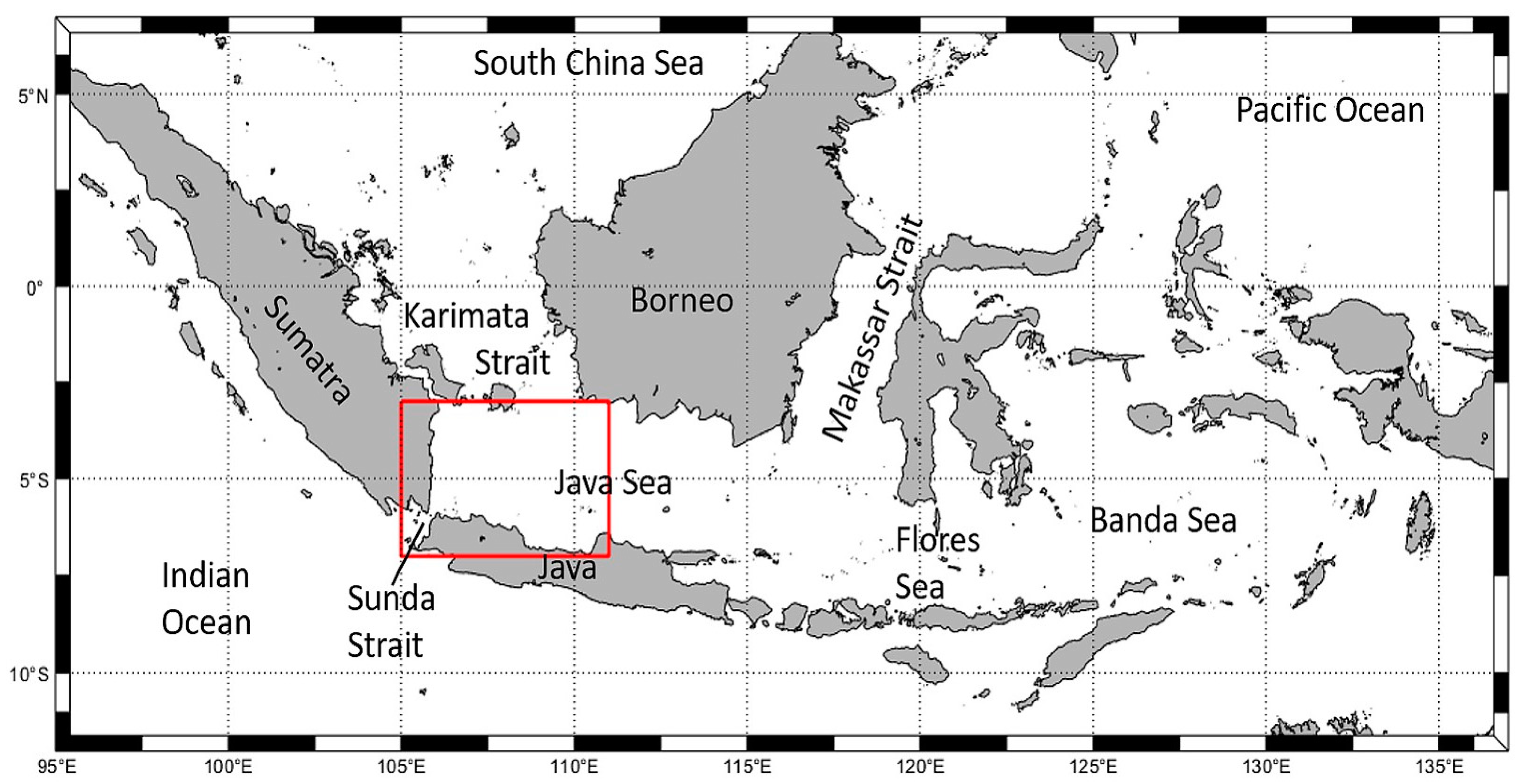
2.1. Region of Interest

The region of interest (ROI) of this study is the Western Java Sea, between 3° S and 7° S and between 105° E and 111° E, as shown by the red rectangle in Figure 1. The borders of the ROI are Sumatra to the West and Java to the South, with the Sunda Strait in between, connecting the Java Sea and the Indian Ocean. The northern border is the Karimata Strait, which forms the connection to the South China Sea. Beyond the ROI, the Java Sea continues towards the east into the Makassar Strait and into the Flores and Banda Seas.

In the ROI, several MPA are located, such as Seribu Islands and Karimun Jawa [25], making the region vulnerable to any kind of oil pollution. At the same time, two major oil production sites are located in the area, off the coasts of western Java and southern Sumatra, and some major shipping routes lead through the Java Sea, connecting the economic centers in China and Japan with Europe, Africa, Australia, and the Persian Gulf. We also chose this region, because it had already been subject to earlier studies [21,26].

The regional climate in the ROI is dominated by the monsoon, resulting in a biannual inversion of the wind direction. From November through March, the northwest monsoon is accompanied by a rainy season, which reaches its peak in January and February. In contrast, the southeast monsoon from May to September is accompanied by a dry season, with lowest precipitation in September. During the transition periods between these two seasons, windspeeds are lower and wind direction changes frequently [27].

2.2. SAR images

The SAR data used were acquired at C-band by the SAR-C aboard Sentinel-1A and Sentinel-1B and by the ASAR aboard ENVISAT, which were launched in 2014, 2016 and 2002, respectively. SAR images from the ROI were downloaded from the Alaska Satellite Facility Distributed Active Archive Center (ASF DAAC) [28]. A total of 1969 Sentinel-1A and -1B SAR images were available from the period from the first provision of Sentinel-1 data in early October 2014 until the end of the 2018/19 northwest monsoon season in late February 2019. These were used for the statistical analysis of oil spills in the ROI.

For each image, we calculated the mean windspeed using reanalysis data from the Copernicus Marine Environment Monitoring Service (CMEMS) [29]. The wind data were provided on a 0.25° × 0.25° grid at a 6-hourly temporal resolution. As oil spills can only be detected in a certain wind speed range [30], any oil pollution statistics can be biased by SAR data acquired under unfavorable wind conditions. In order to avoid such bias, we excluded all SAR data, whose corresponding mean wind speed was lower than 2 m/s or higher than 10 m/s. A total of 85 images were excluded, i.e., 4.3%, because of this criterion. The coverage of the ROI by the remaining 1884 SAR images is shown in Figure 2.

Note that the coverage is highest in the southern and western parts of the ROI, off the coasts of Java and Sumatra, where typical values are between 150 and 200 images. Where different satellite tracks overlap, the coverage may reach 300 images. In contrast, the coverage is rather low in the ROI’s northeast, where typical values range between 50 to 100 images. In this part of the ROI, no SAR images were acquired before 2017, which explains the overall low coverage.

In addition, and to compare results of the visual oil spill detection performed by different operators, we used two sets of SAR images of the ROI: the first was a subset of the above-mentioned Sentinel 1 SAR imagery and consisted of 289 SAR images acquired from October 2014 to February 2017; the second set consisted of 100 ENVISAT ASAR images acquired from May 2006 to February 2012.

Preferably, VV-polarization images were used, because of the higher radar contrast caused by oil pollution [31], and HH-polarization images otherwise. The pixel size of the Sentinel 1 SAR images was 10 m × 10 m and of the ENVISAT SAR images 30 m × 30 m. We recorded the coordinates of the estimated center of each oil spill identified in a SAR image, as well as its length L_s and width W_s.

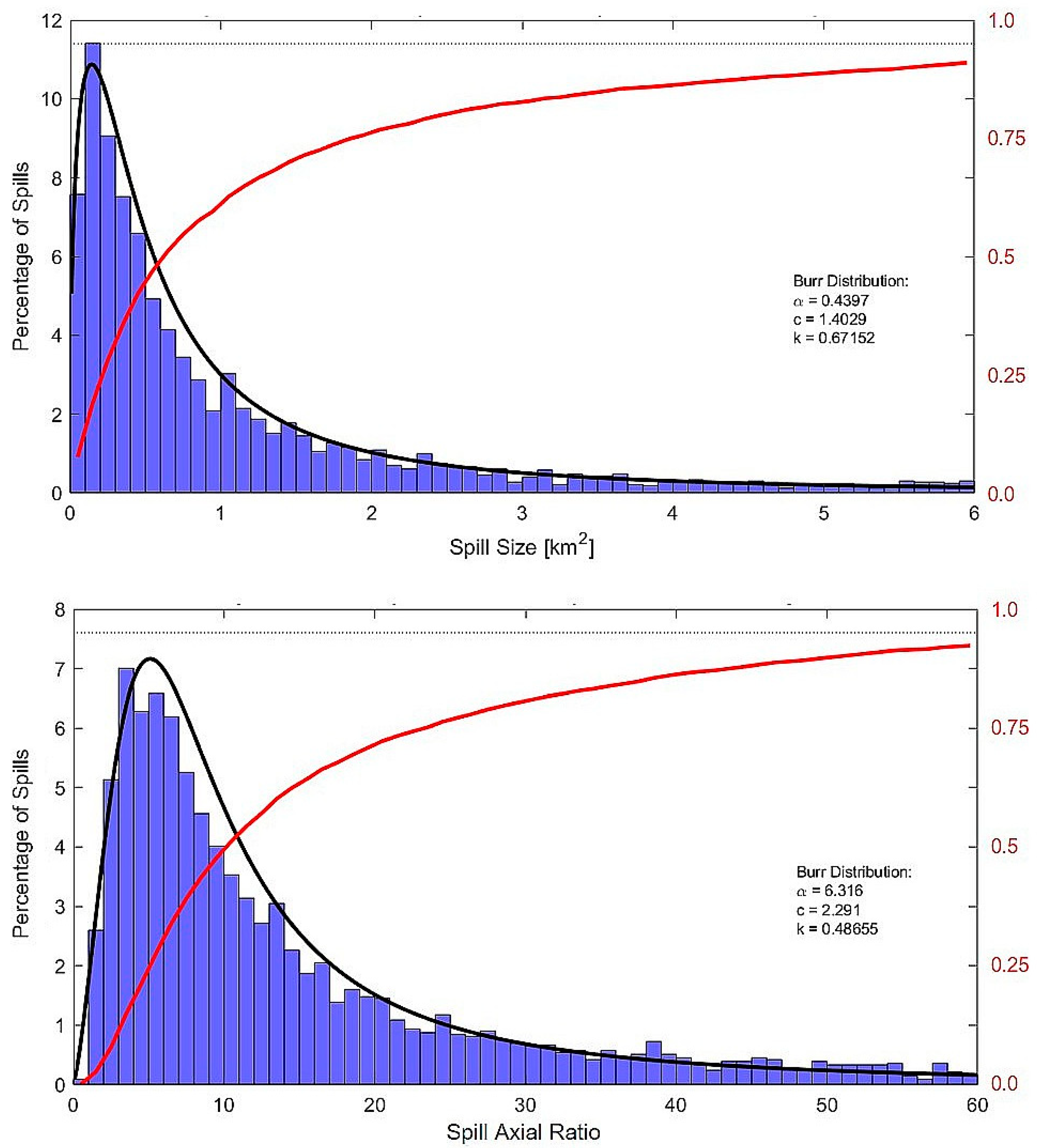
2.3. Statistical Analyses

In order to gain an understanding of the overall distribution of marine oil pollution in the Western Java Sea, we performed statistical analyses of all oil spills found on the SAR images. The inhomogeneous spatial coverage by all SAR images (Figure 2) was taken into account to derive the normalized oil pollution, i.e., the average number of detected oil spills per SAR image, binned into a 0.05° × 0.05° grid. For each grid cell [i;j], the normalized oil pollution, $N_{poll}^{ij}$, was calculated dividing the number of oil spills, whose center coordinates were inside the grid cell, $N_{spills}^{ij}$, by the number of SAR images covering the grid cell, $N_{SAR}^{ij}$:

$$N_{poll}^{ij}=\frac{N_{spills}^{ij}}{N_{SAR}^{ij}}.$$

(1)

The normalized oil pollution, therefore, does not depend on the inhomogeneous SAR coverage. Finally, the recorded length and width were used to calculate the axial ratio, R_s = L_s/W_s, and the spill’s area, A_s, assuming an elliptical shape:

$$A_s=\frac{\pi }{4}·L_s·W_s.$$

(2)

2.4. Different Operators

Analyses of long-term changes in the regional marine oil pollution often require combinations of data sets generated by different operators. In this case, problems may arise when those datasets were generated based on different approaches, or when the operators evaluated the SAR images differently. In order to have an idea of the magnitude of such differences, we compared results from two independent operators, who used the same set of SAR images for their oil spill detection.

The two sets of SAR images, 289 Sentinel-1 SAR-C scenes and 100 ENVISAT ASAR scenes, were analyzed in previous studies [20,21] and were re-evaluated in this paper. All SAR image inspections were performed visually using the Sentinel Application Platform (SNAP) toolbox provided by the European Space Agency (ESA). Care was taken when recorded locations of the spills’ centers were compared because of their uncertainty, which is due to a subjective estimation of center coordinates by different operators. In addition, elongated oil spills, whose SAR signatures were interrupted, might have been interpreted differently, i.e., as two separate spills or as one single spill. Hence, a manual inspection of all datasets was performed and signatures of oil spills with close center coordinates were double checked.

The different datasets, including all parameters recorded for every detected oil spill, were then processed to generate maps of the spills’ spatial distribution and of the mean surface area covered by the spills. Confusion matrices were generated to allow for quantitative estimates of the differences caused by different operators. Finally, we analyzed if a given wind speed range had an effect on the observed differences, e.g., because manifestations of marine oil pollution may have been confused with those of biogenic surface films at lower wind speeds, and if any effect of heavy rain events before the SAR acquisitions can be inferred from our results.

3. Results

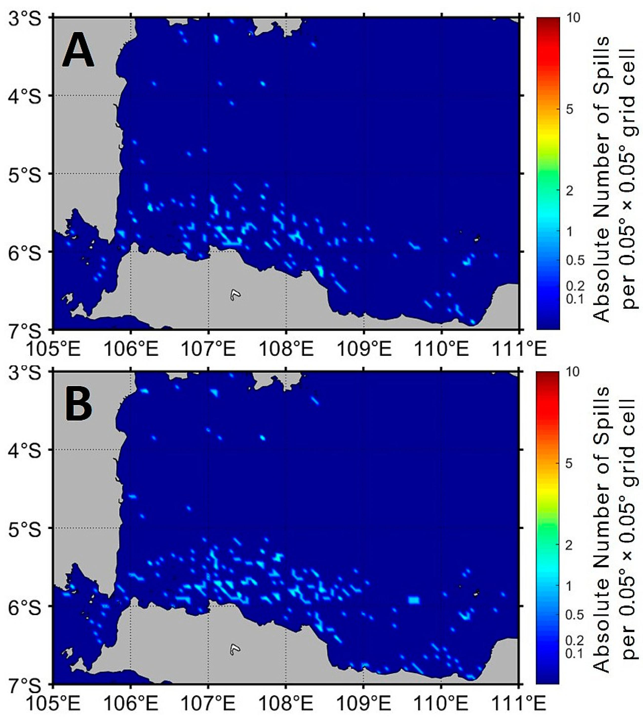
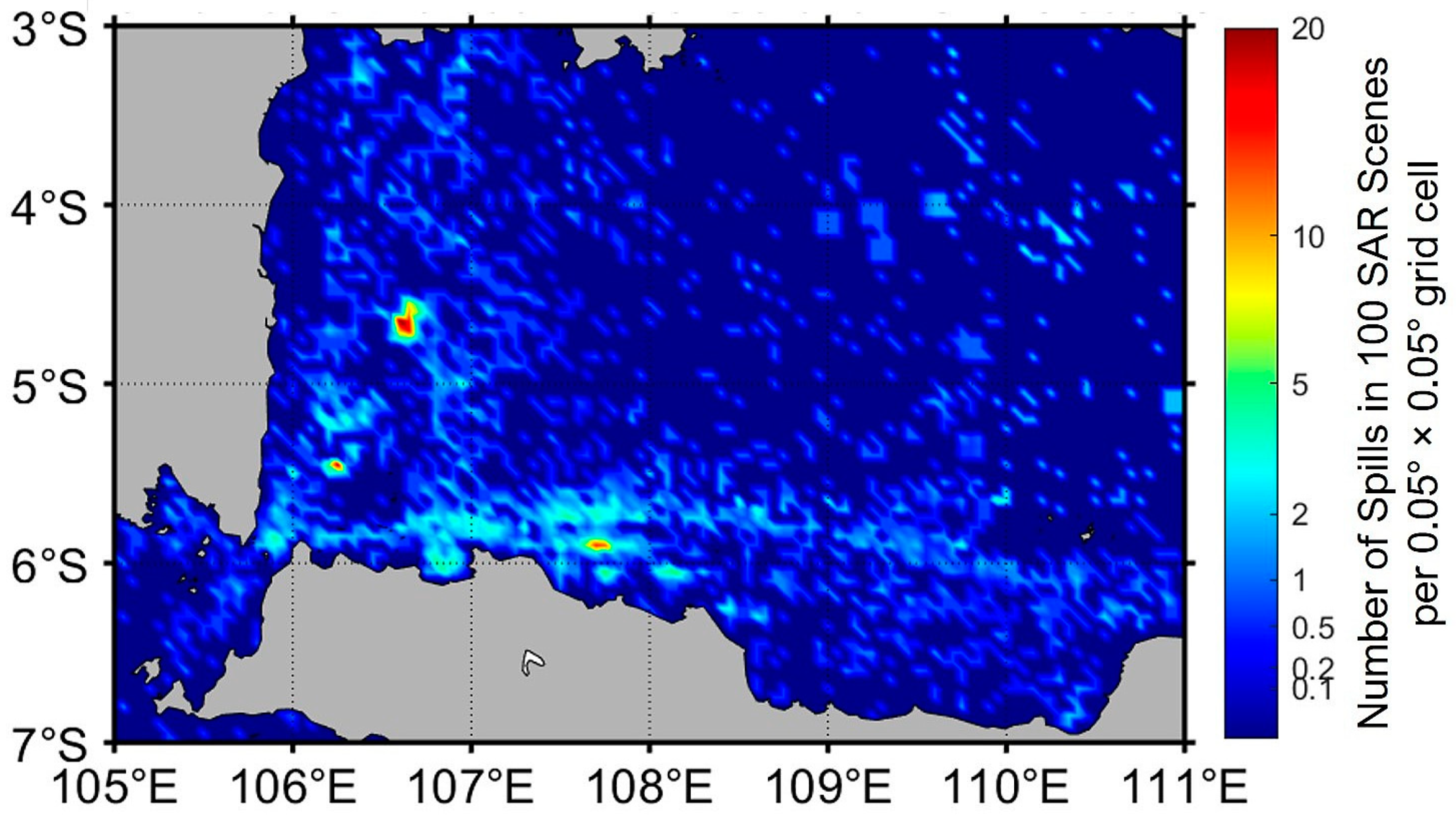
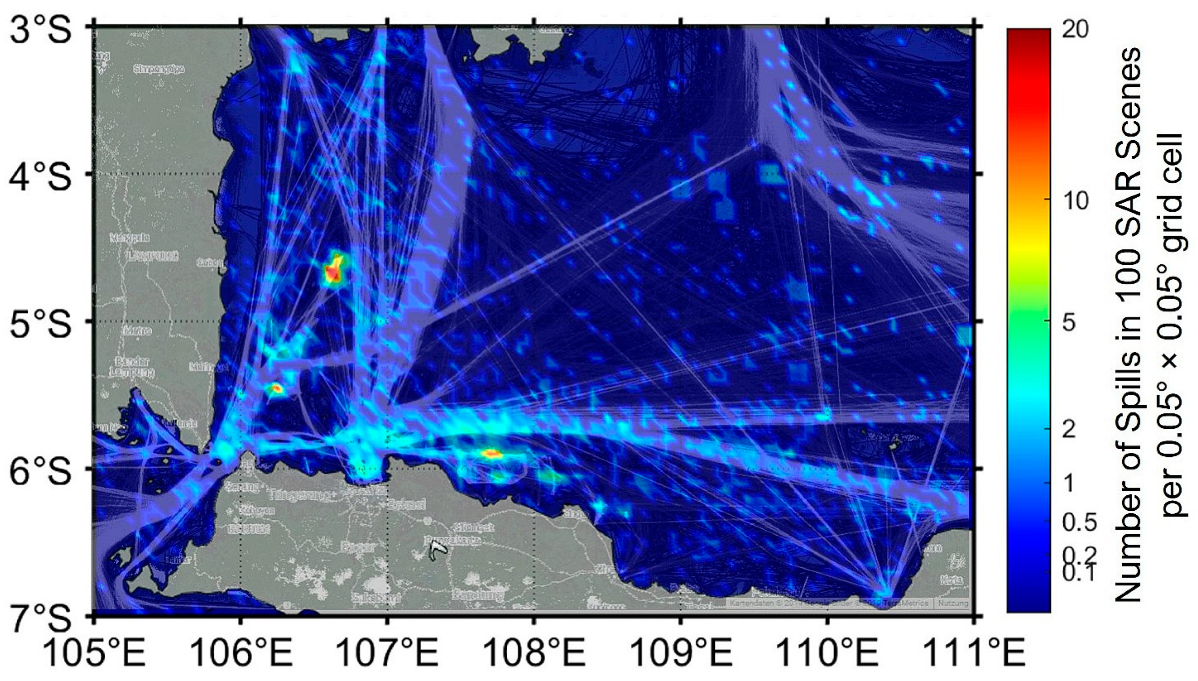
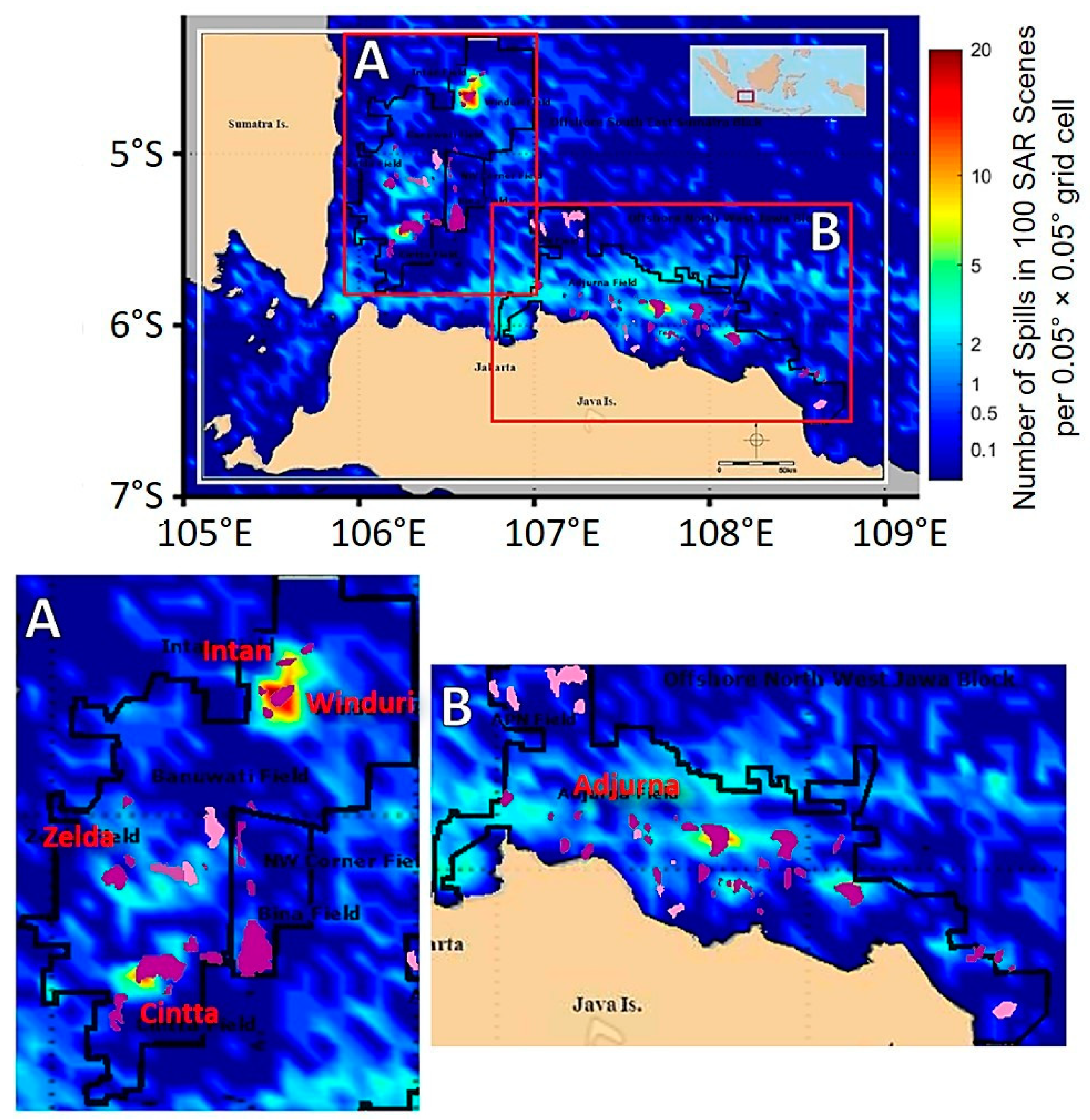
3.1. Spatial Distributions of Oil Spills

On the 1884 Sentinel-1 SAR scenes we evaluated, a total of 3441 oil spills were identified. That is, on average, almost two imprints of oil spills were found on every SAR image acquired in the ROI. The normalized oil pollution, i.e., the spatial distribution of the detected oil spills, derived from those data is shown in Figure 3. Highest numbers of oil spills per 100 SAR scenes were found in coastal regions. Three areas are especially eye-catching, where the normalized oil pollution well exceeds 10 spills per 100 SAR scenes, resulting in red patches on the map shown in Figure 3. Further areas with high numbers of detected oil spills, exceeding 2 spills per 100 SAR scenes (cyan and green colors), were found off western Java (Jakarta Bay) and along a long curved line that connects the Sunda Strait in the west with the central Javanese coast in the east.

We compared these results with a map showing the ship traffic density in 2016 and 2017 [32] and found that most areas of increased normalized oil pollution coincide with the major shipping routes. In Figure 4, those routes are superimposed as pale blue lines to the map of normalized oil pollution, and they can explain the observed high frequency of marine oil pollution in the Sunda Strait, Jakarta Bay, and along the curved line off the Javanese coast. We also note that a narrow shipping route connecting the Sunda Strait and the Karimata Strait in the north leads to higher normalized oil pollution; however, a major route in the north-east of the ROI, which connects the Karimata Strait with the central Java Sea, cannot be inferred from our map, likely because of the low coverage of that area by SAR data (Figure 2). Moreover, the location of major shipping routes cannot explain the observed hot spots, i.e., the red patches on the map.

A more detailed view at the oil production sites Offshore South-East Sumatra (OSES) and Offshore and North-West Java (ONWJ) is provided in Figure 5. In this case, the major oil fields (after [33]) are superimposed as purple patches onto the map of normalized oil pollution, and the major gas fields as pink patches. Within the oil production site OSES (Figure 5A), most spills were found at the oil fields Intan, Winduri, and Cintta (see the red patches in Figure 3). The normalized oil pollution at oil field Zelda is increased, though about four times smaller than at the other oil fields. Within the oil production site ONWJ (Figure 5B), most spills were found in the center of the Adjurna oil field. Note that the above-mentioned curved line of increased normalized oil pollution runs through the northern part of the ONWJ site; hence, higher numbers of oil spills along this line can be attributed to high ship traffic (Figure 4) rather than oil production. Additionally, note that major gas fields, marked as pink patches in all panels of Figure 5, do not coincide with areas of increased normalized oil pollution, unless they are in close vicinity to oil fields.

For each detected oil spill, the lengths of its major and minor axes (i.e., the spill’s length and mean width) were recorded, and they were used to estimate the spill-covered area and the axial ratio (i.e., the inverse compression factor), both assuming an elliptical shape.

Figure 6 shows the respective distributions of the spill size in the upper panel and of the axial ratio in the lower panel. To both distributions, a Burr (Type XII) distribution was fitted (black curves), with the best-fit parameters added to each panel. The Burr (Type XII) distribution is a continuous distribution for non-negative variables and is defined by three parameters, α, c, and k, as [34]:

$$f(x|\alpha ,c,k)=\frac{ck}{\alpha }{\left(\frac{x}{\alpha }\right)}^{c-1}{\left[1+{\left(\frac{x}{\alpha }\right)}^c\right]}^{-k-1}.$$

(3)

In addition, the (inverse) quantile functions were added as red curves, and the horizontal black dotted lines denote the 95% quantile of the respective distribution.

Approximately 50% of the detected oil spills covered sea surface areas smaller than 0.7 km², and about 90% areas smaller than 5.5 km² (upper panel of Figure 6). Neglecting outliers, the mean surface area of the detected oil spills was about 5.6 km², i.e., the largest 10% of the observed oil spills contributed to their mean surface area to an extent comparable to that of the remaining 90%.

The axial ratio of approximately 50% of the detected oil spills was found to be smaller than 11 (lower panel of Figure 6), and that of approximately 90% to be smaller than 50. In most cases, the shape of the observed oil spills was elliptical, with a mean axial ratio of 38, either because of a strong drift of the sea surface layer or a movement of the pollution source, or because of both.

3.2. Comparison of Oil Spill Statistics from Different Operators

In order to obtain an estimate of the influence that the subjective visual interpretation of SAR images has on the detection of oil pollution, we compared results obtained by different operators: in the first case, two independent operators had analyzed 289 Sentinel-1 SAR-C images, and in the second case, a different pair of independent operators had analyzed 100 ENVISAT ASAR images.

3.2.1. First Case: Sentinel-1 Data

The first data set, for which the results obtained by different operators were compared, consisted of 289 Sentinel-1 SAR-C scenes acquired from October 2014 to February 2017 [20]. The same SAR images were re-analyzed, and the location and dimensions of each detected oil pollution were recorded in the same way as performed before. The results of both analyses are compared in

Table 1. Confusion matrix summarizing the results obtained by two independent operators, who analyzed 289 Sentinel 1 SAR-images of the ROI acquired from October 2014 to February 2017.

		Operator 2
	Number of Spills	Detected	Not Detected	∑
Operator 1	Detected	432	369	801
	Not detected	262	-	262
	∑	694	369	1063

.

Operator 1 found a total of 801 oil spills and operator 2 a total of 694 oil spills. Since no a priori knowledge about the real oil pollution, i.e., no sea truth, was available, an exact quantitative assessment of the performance of both operators is not possible. We can, however, make two extreme assumptions, which may indicate if one operator performed better than the other, i.e., if the results obtained by one of the two operators are more reliable than those obtained by the other. We note that both assumptions are simplifying and may not represent the real conditions, i.e., the real amount of oil spills in the ROI. Since no lookalikes (negatives) were recorded, we restrict ourselves to calculations of the hit rate, or recall, R, the precision, P, and the F1 score, F₁, given as [35]:

$$F_1=2\frac{P·R}{P+R}.$$

(4)

In a first simplifying scenario, we may exclude false positives, i.e., we may assume that all detected oil spills were indeed oil pollution, rather than any kind of lookalike, so that both operators produced only true positives and false negatives. Then, a total of 1063 real oil spills were detected by the 2 operators together, of which only 432 (41%) were found by both operators (true positives). Moreover, after missing 262 spills found by operator 2 (false negatives; 25% of all oil spills), the recall (hit rate) of operator 1 would be R₁ = 75% and, vice versa, after missing 369 spills found by operator 1 (false negatives; 35% of all oil spills), the hit rate of operator 2 would be R₂ = 65%. Since the precision P_1,2 of both operators would be 100% (i.e., both produced no false positives), their F1 scores would be F₁₁ = 0.86 (operator 1) and F₁₂ = 0.79 (operator 2).

In another simplifying (extreme) scenario, we may consider as real oil pollution only those oil spills that were found by both operators, so that all spills detected by only one operator are false positives. Then, all 432 oil spills were found by both operators (true positives; both operators had a hit rate of R_1,2 = 100%); operator 1 produced 369 false positives (46% false discovery rate of 801 detected oils spills) and operator 2 produced 262 false positives (38% false discovery rate of 694 detected oil spills). The respective precisions of operators 1 and 2 would be P₁ = 54% and P₂ = 62%, respectively, and hence, their F1 scores would be F₁₁ = 0.70 and F₁₂ = 0.77, respectively.

These two scenarios demonstrate that determining which operator performed better cannot be easily judged. We also note that those extreme scenarios can only be used to obtain rough estimates of the operators’ accuracies, since no ground (sea) truth was available, nor were there any lookalikes (i.e., negatives) recorded.

Whereas quantitative comparisons of the results obtained by different operators are difficult, qualitative comparisons are easier to make. The two panels of Figure 7 show the spatial distributions of the oil spills found by the two operators, with the upper panel (A) showing the results obtained by operator 1, and the lower panel (B) shows the same for operator 2. The overall patterns in both distributions are very similar, and they also agree with those found in the analysis of a greater number of Sentinel-1 SAR images, as described in the previous section. Only small differences in the total number of spills can be found at some locations, e.g., in the Sunda Strait, Jakarta Bay, and in the area of the ONWJ oilfield off the Javanese Coast. These differences are likely to be due to a small number of oil spills identified by one operator only. Note that no spills were detected in the north-eastern part of the ROI, because no SAR images of that area were acquired in the time period considered in this paper (October 2014 to February 2017 [20]).

3.2.2. Second Case: ENVISAT Data

The second data set, for which results obtained by different operators were compared, consisted of 100 ENVISAT ASAR scenes acquired from May 2006 to February 2012 [21]. Again, those SAR images were re-analyzed, and the location and dimensions of each detected oil pollution were recorded in the same way as conducted before. The results of the operators’ analyses are listed as a confusion matrix shown in

Table 2. Confusion matrix summarizing the results obtained by two independent operators, who analyzed 100 ENVISAT ASAR images of the ROI acquired from May 2006 until February 2012.

		Operator 2
	Number of Spills	Detected	Not Detected	∑
Operator 1	Detected	148	32	180
	Not detected	114	-	114
	∑	262	32	294

. In total, operator 1 found 180 oil spills, and operator 2 found 262 oil spills; 148 oil spills were identified by both operators, and the overall sum of spills identified by the two operators together was 294.

In the first scenario, again, we assume that there were no false positives, i.e., that all identified oil spills were indeed caused by oil pollution. Then, only 50% of all oil spills were found by both operators; the hit rate of operator 1 would be R₁ = 61%, since 114 oil spills were missed (false negatives; false discovery rate 39%), and the hit rate of operator 2, who missed 32 spills (false negatives; false discovery rate 11%), would be R₂ = 89%. The precisions of both operators would again be P_1,2 = 100% and hence, their respective F1 scores would be F₁₁ = 0.76 (operator 1) and F₁₂ = 0.94 (operator 2).

In the second scenario, again, only those 148 oil spills, which were found by both operators (Table 2), are considered as true positives. The hit rates of both operators would again be R_1,2 = 100%, without any false negatives; the false discovery rate of operator 1 would be 18% (32 of 180 detected oil spills), and the false discovery rate of operator 2 would be 44% (114 of 262 detected oil spills). The respective precisions of operators 1 and 2 would be P₁ = 82% and P₂ = 56%, respectively, and hence, their F1 scores would be F₁₁ = 0.90 and F₁₂ = 0.72, respectively.

We note that none of the operators is performing better, achieving a higher F1 score, in both extreme scenarios, as it was already found in the previous section. We also note that even in the first scenarios, both operators may have missed some oil spills, which, naturally, would result in lower F1 scores. Further, as no negatives (lookalikes) were recorded, the above statical assessment must remain simplified.

The two panels of Figure 8 show the spatial distribution of the oil spills found by the two operators, with the results obtained by operator 1 shown in the upper panel (A) and the results obtained by operator 2 shown in the lower panel (B). Similar to the results presented in Figure 7, the overall patterns of the detected oil spills are the same for both operators. Because of the overall larger number of oil spills found by operator 2 (Table 2), more bright patches can be seen in the lower panel; however, they do not affect the good qualitative agreement between both data sets.

3.3. Influence of Weather Conditions

The visibility of oil pollution on SAR imagery depends, among others, on the prevailing weather conditions. We analyzed the datasets with respect to the influence that the wind speed range and preceding rain events have on the detectability of oil spills.

3.3.1. Wind Speed Range

The previous section demonstrated that large differences can be found between results obtained by different operators. A reason for the observed differences can be that small oil spills, whose imprints may cover only a few SAR image pixels, were missed by one of the operators. Another possible reason is that oil spills were confused with lookalikes, especially biogenic surface films, or vice versa. Such erroneous classifications may have happened, when SAR images were analyzed that were acquired at low-to-moderate wind speeds, when both types of surface films cause similar radar contrasts [31]. While mineral oil spills can be detected on SAR images at wind speeds up to 10 m/s [30], the upper limit of wind speeds, at which biogenic surface films are manifested on SAR images, is about 7 m/s [36,37].

To investigate if the observed differences caused by different operators depend on the chosen wind speed range, we re-analyzed the given results, but considered only those SAR images that were acquired at higher wind speeds, by raising the lower wind speed limit from 2 m/s to 5 m/s. In this subset of SAR images less manifestations of biogenic surface films can be expected and therefore, the risk of misinterpretations should be reduced. Moreover, since small oil spills have a shorter lifetime at high wind speeds, the average spill size should increase and therefore, the risk of being overseen by an operator should decrease. We note that a further increase in the lower wind speed limit would have resulted in a too small number of (remaining) oil spills, thereby hindering a significant analysis.

In

Table 3. Percentage of spills found by both operators, and the mean area of spills not found by one operator, in 289 Sentinel-1 SAR-C scenes acquired from October 2014 to February 2017, applying different lower limits of the wind speed range (see text).

Wind Speed Range (m/s)	Percentage of Spills Found by Both Operators	Mean Area of Spills Missed by One Operator (km2)
2–10	41	1.08
5–10	50	0.94

and

Table 4. Same as Table 3, but for 100 ENVISAT ASAR scenes acquired from May 2006 to February 2012.

Wind Speed Range (m/s)	Percentage of Spills Found by Both Operators	Mean Area of Spills Missed by One Operator (km2)
2–10	48	1.81
5–10	63	4.22

, the results are shown for the Sentinel-1 dataset and for the ENVISAT dataset, respectively. Both tables list for the two wind speed ranges the percentages of oil spills found by both operators, along with the mean area of the spills that were not found by both operators, i.e., that were missed by one operator.

In both data sets, the percentage of oil spills found by both operators increased when the lower wind speed limit was raised: in the Sentinel-1 dataset, the increase was 9 percentage points, and in the ENVISAT dataset 15 percentage points. These results support our hypothesis that the confusion of oil spills and biogenic surface films is a main source of uncertainty in the SAR image analysis.

The mean area of spills, which were not detected by both operators, slightly decreased in the Sentinel-1 dataset, but it strongly increased in the ENVISAT dataset. Apparently, most of the small oil spills on Sentinel-1 SAR-C images, which were not detected by one of the operators when the lower wind speed limit was 2 m/s, were also missed when the lower limit was raised to 5 m/s. In contrast, the mean area of small spills on ENVISAT ASAR images more than doubled when the lower wind speed limit was raised from 2 m/s to 5 m/s. However, since there was no general trend observed in both datasets, our hypothesis, that the mean area should generally increase, is not supported by these results. We also note that different pairs of operators analyzed the two datasets, that the sizes of the two datasets were different, and that their pixel sizes differed by a factor of three, which altogether makes it difficult to draw final conclusions.

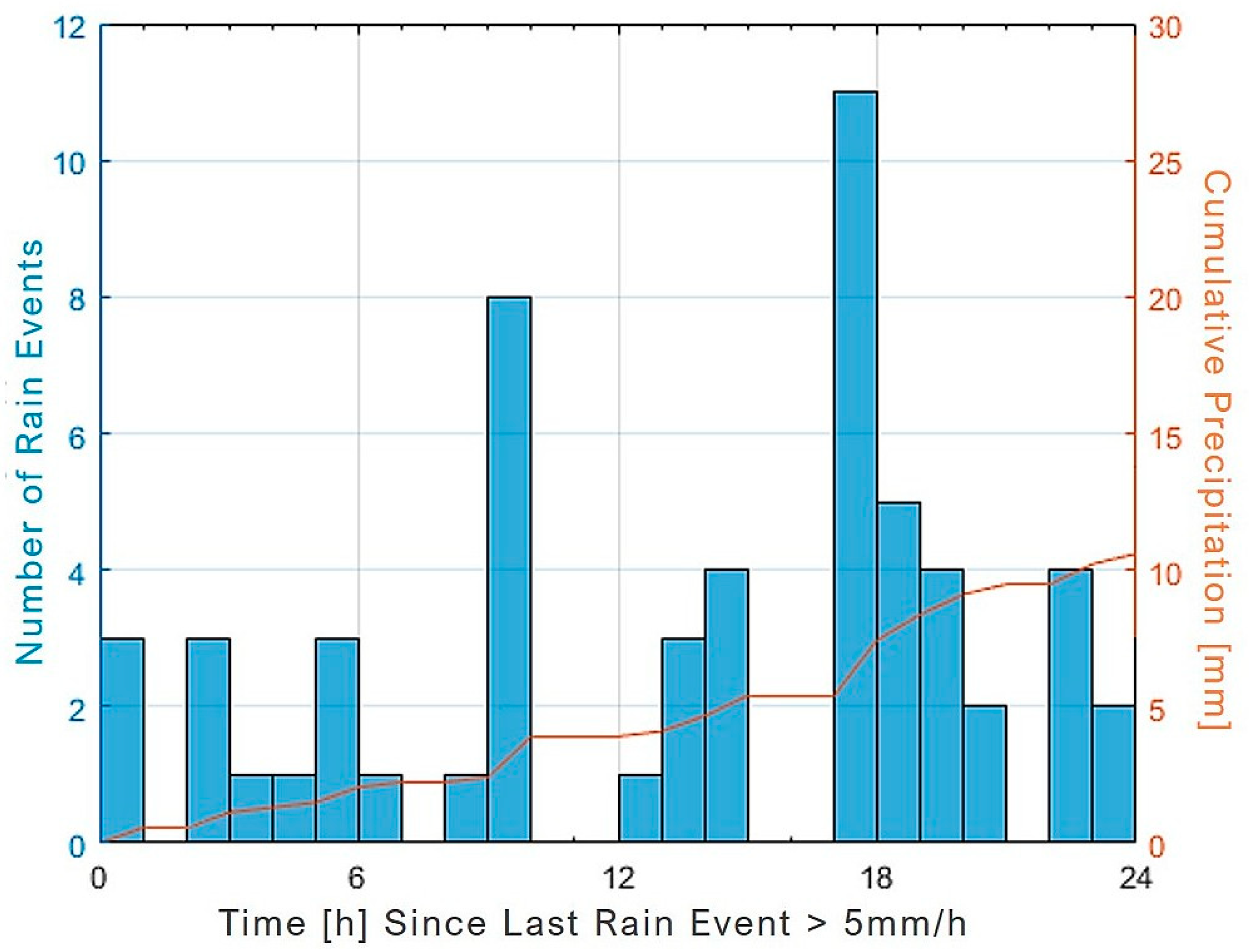
3.3.2. Heavy Rain Events

Heavy rain disrupts marine surface films [38], and it takes some time until a coherent film has formed again on the sea surface. As a result, the time between a heavy rain event and the SAR image acquisition may affect the detectability of oil pollution. We used the datasets from [21] to investigate if heavy precipitation with rain rates exceeding 5 mm/h may affected the results presented in this paper. For every detected oil spill, we calculated the time between the respective SAR image acquisition and the latest heavy rain event using reanalysis data from the Copernicus Climate Data Storage (CDS) [39], which are provided on a 0.25° × 0.25° grid at an hourly temporal resolution. The temporal distribution is shown in Figure 9.

Two maxima in the temporal distribution can be seen, at 10 h and 18 h, which are likely to be due to heavy convective precipitation in the afternoon hours. There is, however, no clear trend visible, which would indicate that a certain time period between the latest strong rainfall and the SAR image acquisition is needed to allow for a detection of oil pollution on the SAR imagery. Apparently, a larger data basis is needed to draw definite conclusions. We also note that the spatio-temporal resolution of the reanalysis data might be too low, since the oil spills may form again at the sea surface within the first hour after the rainfall, and since tropical rain cells are often of sizes 2–40 km [40] and are not resolved by the used reanalysis data.

4. Discussion

Our results on the spatial distribution of marine oil pollution in the Western Java Sea confirm those from earlier studies [20,21], as similar overall pollution patterns were found. Most of the oil spills were detected along major shipping routes and in close vicinity to oil production sites. Other regions where a higher-than-average number of oil spills can be found, such as popular fishing grounds or near the shore especially at river outflows, [17] were not included in the analysis. However, most pollution that was found near the coast is located close to harbors. The most prominent example in our results is in Jakarta Bay, where one the busiest Indonesian harbors is located. There are also harbors on both sides of the Sunda Strait, which are connected by frequent traffic and smaller harbors along the Javanese coast. Near all these harbors, oil pollution was repeatedly found close to the coast.

Moreover, the majority of the detected oil spills was smaller than 1 km², and most oil spills were of elliptical shape, with an axial ratio smaller than 10. We did not find a correlation between spill sizes and axial ratios. It is however likely that a large number of small oil spills were not found, particularly on ENVISAT ASAR images, whose spatial resolution is three times lower than that of the Sentinel-1 SAR-C images. The different spatial resolutions may also explain why a larger quantity of small oil spills, with sizes smaller than 0.5 km², were found on Sentinel-1 SAR-C images. We further note that the highest normalized oil pollution, i.e., the largest number of oil spills per 100 SAR scenes and per grid cell, was found at the major oil fields.

The visual analyses performed by different operators revealed the same qualitative result, that the overall patterns in the oil pollution are the same. However, not even half of the spills were found by two operators, who were independently analyzing the same set of SAR images. The percentage of spills found by both operators increased by approximately 10 percentage points when only SAR images were considered, which were acquired at higher wind speeds. That is, by raising the lower wind speed limit from 2 m/s to 5 m/s, we reduced the risk that biogenic surface films were mistaken for oil spills, because the latter are more likely to be disrupted at higher wind speeds than oil spills [30,37]. These differences confirm the results of a similar study, in which two operators classified 7 out of 22 oil spills found with the same confidence level, where the confidence level depended, among other factors, on the wind speed [19].

Based on 289 Sentinel-1 SAR-C images, the mean area of those oil spills that were not found by both operators was slightly reduced when a higher wind speed range was considered. In contrast, the mean area of the oil spills, which were not found by both operators on 100 ENVISAT ASAR images, increased considerably when the lower wind speed limit was raised. Only the latter result supports our assumption that differences in the results obtained by different operators are caused by confusion of oil spills and lookalikes, such as biogenic surface films, especially for large, elongated spills. Further comparisons based on larger quantities of SAR images are needed to draw definite conclusions.

Even though the differences in the results obtained by different operators could be reduced by raising the lower wind speed limit, they are still too large to allow for a seamless combination. This is especially true when the development of oil pollution over time is investigated. For qualitative studies of oil pollution in a given area, these differences are less important, as the overall patterns of detected oil pollution do not depend on the operator. It must also be considered that the classification of dark patches into oil spills or lookalikes may change over time, as a single operator gains more experience in SAR image analysis, and particularly in distinguishing dark patches of different origin. Additionally, the detail, at which said operator inspects the SAR images can vary from day to day or even from image to image, even if the operator endeavors to keep the given efforts on a constant (high) level.

This study is however based on a small number of SAR images and therefore, our results cannot be easily applied to other datasets. For more significant conclusions on the influence that different operators have on oil pollution statistics, further studies employing larger datasets examined by more than two operators are needed.

5. Conclusions

For our statistical analyses, a total of 1969 Sentinel 1 SAR-C scenes of the Western Java Sea acquired from October 2014 to February 2019 were visually inspected with regard to imprints of marine oil pollution. The results of the spatial analysis show that most spills were found along major shipping routes and at oil production sites. Approximately half of the spills have an area smaller than 1 km² and have an axis ratio smaller than 10; however, oil spills over six times that size were also found.

When comparing the results from independent operators examining the same set of SAR images, we found that there are quantitative differences while the overall patterns of marine oil pollution were the same. The percentage of spills, which were found by both operators, increased when the lower limit of the wind speed range was raised, for which SAR imagery was considered. Our results indicate that fewer biogenic surface films were mistaken for oil spills at higher wind speeds, because of the different wind speed ranges, at which both types of surface films manifest on SAR imagery. Moreover, the fact that small oil spills can be easily missed appears to be a major source for differences in the results from two operators.

Oil pollution statistics based on visual observations of SAR imagery may be used as training datasets for automated oil pollution detection systems. Hence, our results are important for an assessment of potential errors in those systems. Further research in this respect will be conducted. Future research will also see an investigation of radar polarization (VV vs. HH) on the detection performance for low wind conditions and incidence angle.

References

1. Andrews, N.; Bennett, N.J.; Le Billon, P.; Green, S.J.; Cisneros-Montemayor, A.M.; Amongin, S.; Gray, N.J.; Sumaila, U.R. Oil, fisheries and coastal communities: A review of impacts on the environment, livelihoods, space and governance. Energy Res. Soc. Sci. 2021, 75, 102009. [Google Scholar] [CrossRef]
2. BP. BP Statistical Review of World Energy 68th Edition. Available online: https://www.bp.com/content/dam/bp/business-sites/en/global/corporate/pdfs/energy-economics/statistical-review/bp-stats-review-2019-full-report.pdf (accessed on 13 January 2020).
3. Ferraro, G.; Meyer-Roux, S.; Muellenhoff, O.; Pavliha, M.; Svetak, J.; Tarchi, D.; Topouzelis, K. Long term monitoring of oil spills in European seas. Int. J. Remote Sens. 2009, 30, 627–645. [Google Scholar] [CrossRef]
4. Wahl, T.; Skøelv, Å.; Pedersen, J.P.; Seljelv, L.-G.; Andersen, J.H.; Follum, O.A.; Anderssen, T.; Strøm, G.D.; Bern, T.-I.; Espedal, H.H.; et al. Radar satellites: A new tool for pollution monitoring in coastal waters. Coast. Manag. 1996, 24, 61–71. [Google Scholar] [CrossRef]
5. ESA. Oil Pollution Monitoring. In ESA Brochure BR-128/I: ERS and its Applications: Marine; Calabresi, G., Bellini, A., Battrick, B., Eds.; 1998; p. 64. Available online: https://www.esa.int/esapub/br/br128/br128_1.pdf (accessed on 10 February 2022).
6. Fingas, M.; Brown, C.E. A Review of Oil Spill Remote Sensing. Sensors 2018, 18, 91. [Google Scholar] [CrossRef] [PubMed] [Green Version]
7. Cheng, Y.; Li, X.; Xu, Q.; Garcia-Pineda, O.; Andersen, O.B.; Pichel, W.G. SAR observation and model tracking of an oil spill event in coastal waters. Mar. Pollut. Bull. 2011, 62, 350–362. [Google Scholar] [CrossRef]
8. Brekke, C.; Solberg, A.H.S. Oil spill detection by satellite remote sensing. Remote Sens. Environ. 2005, 95, 1–13. [Google Scholar] [CrossRef]
9. Gade, M. On the imaging of biogenic and anthropogenic surface films on the sea by radar sensors. In Marine Surface Films: Chemical Characteristics, Influence on Air-Sea Inter-actions and Remote Sensing; Gade, M., Hühnerfuss, H., Korenowski, G.M., Eds.; Springer: Berlin/Heidelberg, Germany, 2006; pp. 189–204. [Google Scholar]
10. Migliaccio, M.; Gambardella, A.; Tranfaglia, M. SAR Polarimetry to Observe Oil Spills. IEEE Trans. Geosci. Remote Sens. 2007, 45, 506–511. [Google Scholar] [CrossRef]
11. Espedal, H. Detection of oil spill and natural film in the marine environment by spaceborne SAR. In Proceedings of the International Symposium on Geoscience and Remote Sensing (IGARSS) 1999, Hamburg, Germany, 28 June– 2 July 1999; pp. 1478–1480. [Google Scholar]
12. Fiscella, B.; Giancaspro, A.; Nirchio, F.; Pavese, P.; Trivero, P. Oil Spill detection using marine SAR images. Int. J. Remote Sens. 2000, 21, 3561–3566. [Google Scholar] [CrossRef]
13. Leifer, I.; Lehr, W.J.; Simecek-Beatty, D.; Bradley, E.; Clark, R.; Dennison, P.; Hu, Y.; Matheson, S.; Jones, C.E.; Holt, B.; et al. State of the art satellite and airborne marine oil spill remote sensing: Application to the BP Deepwater Horizon oil spill. Remote Sens. Environ. 2012, 124, 185–209. [Google Scholar] [CrossRef] [Green Version]
14. Wang, Z.; An, C.; Lee, K.; Owens, E.; Chen, Z.; Boufadel, M.; Taylor, E.; Feng, O. Factors influencing the fate of oil spilled on shorelines: A review. Environ. Chem. Lett. 2021, 19, 1611–1628. [Google Scholar] [CrossRef]
15. Solberg, A.; Storvik, G.; Solberg, R.; Volden, E. Automatic detection of oil spills in ERS SAR images. IEEE Trans. Geosci. Remote Sens. 1999, 37, 1916–1924. [Google Scholar] [CrossRef] [Green Version]
16. Topouzelis, K.; Psyllos, A. Oil spill feature selection and classification using decision tree forest on SAR image data. ISPRS J. Photogramm. Remote Sens. 2012, 68, 135–143. [Google Scholar] [CrossRef]
17. Cao, Y.; Xu, L.; Clausi, D. Exploring the Potential of Active Learning for Automatic Identification of Marine Oil Spills Using 10-Year (2004–2013) RADARSAT Data. Remote Sens. 2017, 9, 1041. [Google Scholar] [CrossRef] [Green Version]
18. Zhang, Y.; Li, Y.; Liang, X.S.; Tsou, J. Comparison of Oil Spill Classifications Using Fully and Compact Polarimetric SAR Images. Appl. Sci. 2017, 7, 193. [Google Scholar] [CrossRef] [Green Version]
19. Solberg, A.S. Automatic Detection and Estimating Confidence for Oil Spill Detection in SAR Images. In Proceedings of the 21st International Symposium on Remote Sensing of Environment (ISRSE), St. Petersburg, Russian, 20–24 June 2005. [Google Scholar]
20. Meier, C. Untersuchungen zur Detektion von Mariner Ölverschmutzung in Indonesischen Seegebieten mit Satellitengestützten Radarsensoren. Bachelor’s Thesis, Universität Hamburg, Fachbereich Geowissenschaften, Hamburg, Germany, 2016. [Google Scholar]
21. Gade, M.; Mayer, B.; Meier, C.; Pohlmann, T.; Putri, M.; Setiawan, A. An assessment of marine oil pollution in Indonesia based on SAR imagery. In Proceedings of the IEEE Intern. Geosci. Remote Sens. Sympos. (IGARSS) 2017, Fort Worth, TX, USA, 23–28 July 2017; pp. 1534–1537. [Google Scholar]
22. Lu, J. Marine oil spill detection, statistics and mapping with ERS SAR imagery in south-east Asia. Int. J. Remote Sens. 2003, 24, 3013–3032. [Google Scholar] [CrossRef]
23. Ivanov, A.; He, M.-X.; Fang, M. Oil spill detection with the RADARSAT SAR in the waters of the Yellow and East China Sea: A case study. In Proceedings of the 23rd Asian Conference on Remote Sensing, Kathmandu, Nepal, 25–29 November 2002; pp. 25–29. [Google Scholar]
24. Mohr, V. Satellitengestützte Radar-Fernerkundung mariner Ölverschmutzung in der Javasee. Bachelor’s Thesis, Universität Hamburg, Fachbereich Geowissenschaften, Hamburg, Germany, 2019. [Google Scholar]
25. Setiawan, A.; Putri, M.R.; Gade, M.; Pohlmann, T.; Mayer, B. Combining ocean numerical model and SAR imagery to investigate the occurrence of oil pollution, a case study for the Java Sea. IOP Conf. Ser. Earth Environ. Sci. 2017, 54, 12080. [Google Scholar] [CrossRef] [Green Version]
26. Barale, V.; Gade, M. Remote Sensing of the Asian Seas; Springer International Publishing: Cham, Switzerland, 2019; ISBN 978-3-319-94065-6. [Google Scholar]
27. Durand, J.-R.; Petit, D. The Java Sea Environment. In Biodynex: Biology, Dynamics, Exploitation of the Small Pelagic Fishes in the Java Sea; Potier, M., Nurhakim, S., Eds.; Agency for Agricultural Research and Development: Jakarta, Indonesia, 1995. [Google Scholar]
28. Alaska Satellite Facility Distributed Active Archive Center (ASF DAAC). Available online: https://search.asf.alaska.edu (accessed on 4 August 2019).
29. Copernicus Marine Environment Monitoring Service (CMEMS). Available online: https://marine.copernicus.eu (accessed on 4 August 2019).
30. Gade, M.; Alpers, W. Using ERS-2 SAR images for routine observation of marine pollution in European coastal waters. Sci. Total Environ. 1999, 237–238, 441–448. [Google Scholar] [CrossRef]
31. Gade, M.; Alpers, W.; Hühnerfuss, H.; Masuko, H.; Kobayashi, T. The imaging of biogenic and anthropogenic surface films by a multi-frequency multi-polarization synthetic aperture radar measured during the SIR-C/X-SAR missions. J. Geophys. Res. 1998, 103, 18851–18866. [Google Scholar] [CrossRef]
32. Marine Traffic. Available online: http://marinetraffic.com (accessed on 16 October 2019).
33. Mande. Offshore North West Java (ONWJ). Mande Blog on wordpress.com. Available online: https://ngsuyasa.wordpress.com/2014/03/13/offshore-north-west-java-onwj-block-at-java-sea/ (accessed on 17 October 2019).
34. Burr, I.W. Cumulative frequency functions. Ann. Math. Stat. 1942, 13, 215–232. [Google Scholar] [CrossRef]
35. Chinchor, N. MUC-4 Evaluation Metrics. In Proceedings of the Fourth Mess. Underst. Conf. (MUC-4), McLean, VA, USA, 16–18 June 1992; pp. 22–29. [Google Scholar]
36. Gade, M.; Byfield, V.; Ermakov, S.; Lavrova, O.; Mitnik, L. Slicks as Indicators for Marine Processes. Oceanography 2013, 26, 138–149. [Google Scholar] [CrossRef] [Green Version]
37. Espedal, H.A. Satellite SAR oil spill detection using wind history information. Int. J. Remote Sens. 1999, 20, 49–65. [Google Scholar] [CrossRef]
38. Green, T.; Houk, D.F. The removal of organic surface films by rain. Limnol. Ocean. 1979, 24, 966–970. [Google Scholar] [CrossRef]
39. Copernicus Climate Data Storage (CDS). Available online: https://cds.climate.copernicus.eu (accessed on 9 October 2019).
40. Holt, B. SAR Imaging of the Ocean Surface. In SAR Marine User’s Manual; Jackson, C.R., Apel, J.R., Eds.; NOAA: Washington, DC, USA, 2004; pp. 25–80. [Google Scholar]
Figure 1. Map of Indonesia with the region of interest marked by the red rectangle.
Remotesensing 14 00880 g001
Figure 2. Coverage of the ROI in the Western Java Sea by Sentinel 1 SAR images acquired from October 2014 to February 2019.
Remotesensing 14 00880 g002
Figure 3. Normalized oil pollution in the ROI. The number of oil spills found on 1884 Sentinel SAR-C scenes acquired from October 2014 to February 2019 was normalized by the SAR coverage and binned into a 0.05° × 0.05° grid.
Remotesensing 14 00880 g003
Figure 4. Same as Figure 3, with the main shipping routes superimposed (after [32], original data © Marine Traffic).
Remotesensing 14 00880 g004
Figure 5. Same as Figure 3, but with a focus on major oil production sites; A: ‘Offshore North-East Sumatra’; B: ‘Offshore North-West Java’. Purple patches mark the locations of oil fields, and pink patches mark the locations of gas fields (redrawn after [33]).
Remotesensing 14 00880 g005
Figure 6. Distribution of the size (upper panel) and axial ratio (lower panel) of 3441 oil spills detected on 1884 Sentinel SAR-C scenes acquired from October 2014 to February 2019. Added to each histogram are the best-fit Burr distributions (black) and the (inverse) quantile functions (red); the horizontal dotted line marks the 95% quantile.
Remotesensing 14 00880 g006
Figure 7. Comparison of the absolute numbers of oil spills per 0.05° × 0.05° grid cell found by two different operators on 289 Sentinel-1 scenes acquired from October 2014 to February 2017. A: operator 1; B: operator 2.
Remotesensing 14 00880 g007
Figure 8. Same as Figure 7, but based on 100 ENVISAT ASAR scenes acquired from May 2006 to February 2012.
Remotesensing 14 00880 g008
Figure 9. Heavy precipitation events prior to SAR image acquisitions. The bars indicate the temporal distribution of heavy rain events (>5 mm/h) at the location of detected oil spills; the orange line represents the cumulative precipitation.
Remotesensing 14 00880 g009