
Spatial Stratification Method for the Sampling Design of LULC Classification Accuracy Assessment: A Case Study in Beijing, China


Abstract
:
1. Introduction
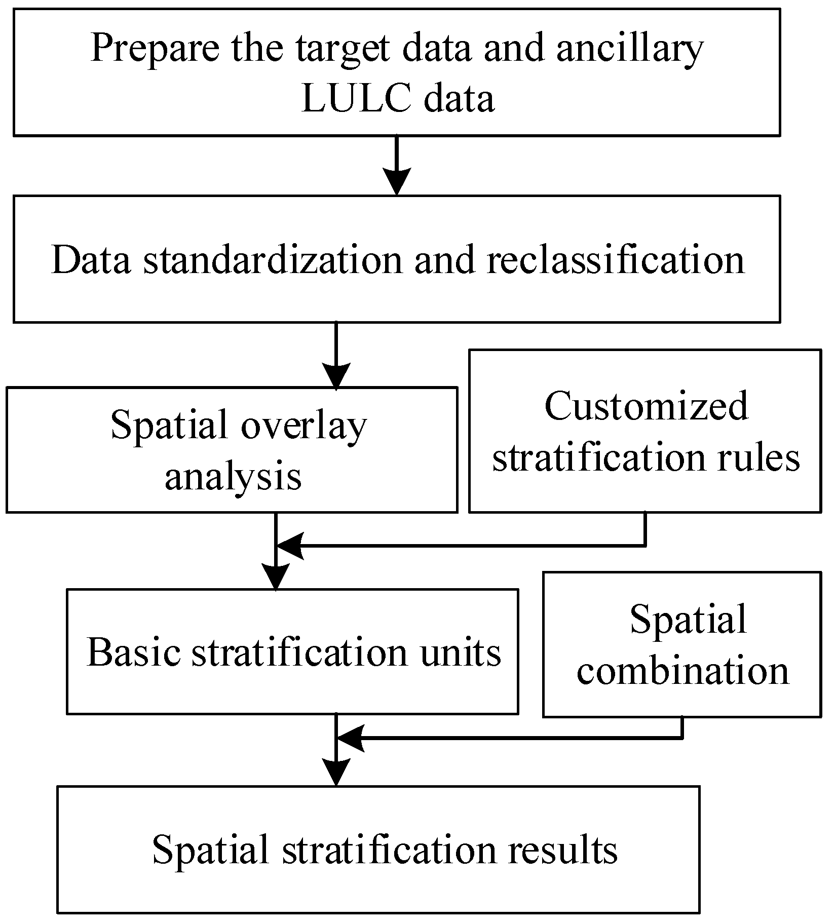
2. Spatial Stratification Method
3. Case Study
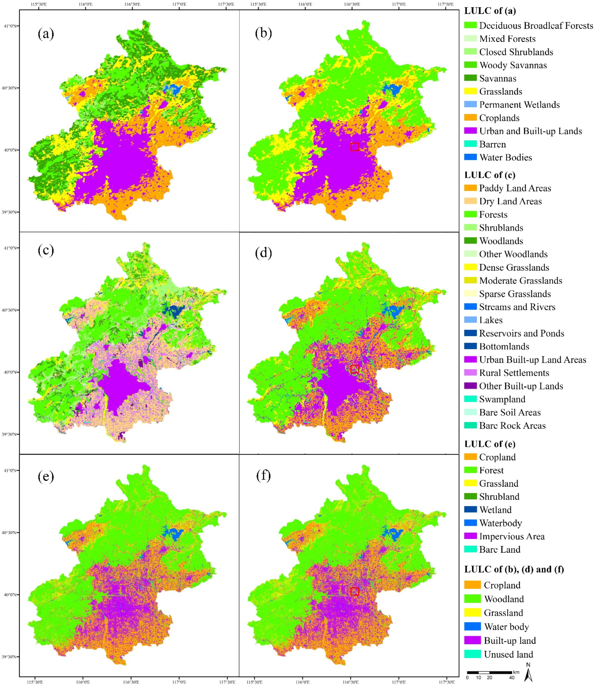
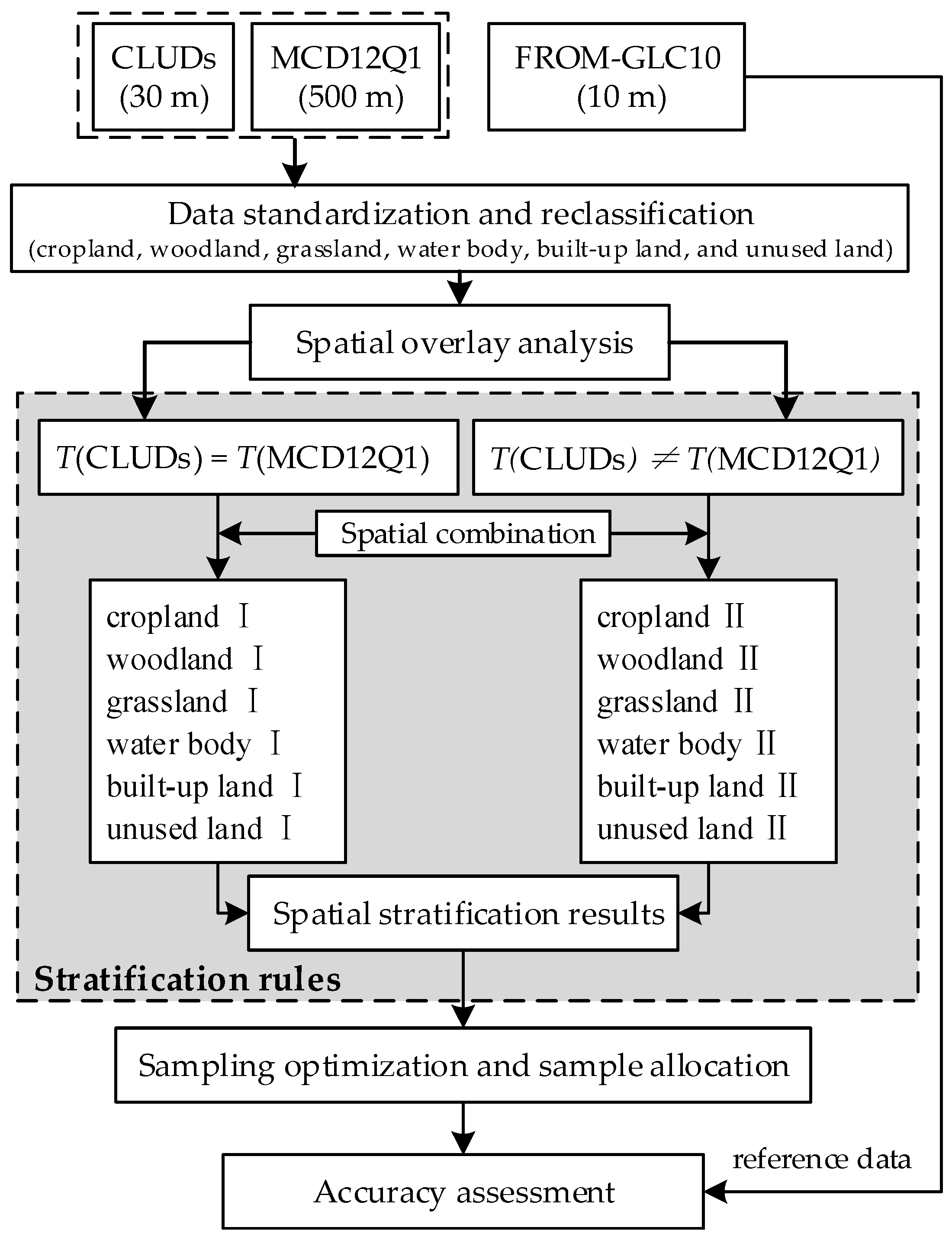
3.1. Data Sources and Experiment Roadmap
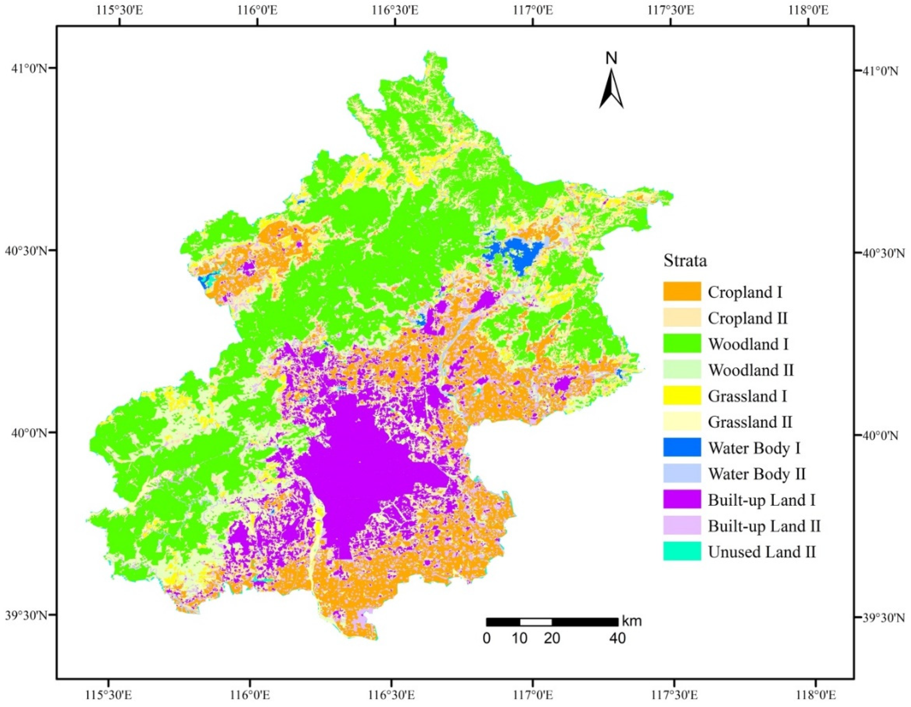
3.2. Spatial Stratification
3.3. Sampling Optimization
3.4. Comparative Metrics for Accuracy Assessment
4. Results
4.1. Spatial Stratification of CLUDs and MCD12Q1 for Beijing
4.2. Sampling Optimization and Sample Allocation
4.3. Accuracy Assessment of CLUDs Using FROM-GLC10 and Comparative Analysis
5. Discussion
6. Conclusions
Author Contributions
Funding
Institutional Review Board Statement
Informed Consent Statement
Data Availability Statement
Acknowledgments
Conflicts of Interest
References
- Searchinger, T.D.; Wirsenius, S.; Beringer, T.; Dumas, P. Assessing the efficiency of changes in land use for mitigating climate change. Nature 2018, 564, 249–253. [Google Scholar] [CrossRef] [PubMed]
- Stehfest, E.; van Zeist, W.J.; Valin, H.; Havlik, P.; Popp, A.; Kyle, P.; Tabeau, A.; Mason-D’Croz, D.; Hasegawa, T.; Bodirsky, B.L.; et al. Key determinants of global land-use projections. Nat. Commun. 2019, 10, 2166. [Google Scholar] [CrossRef] [PubMed] [Green Version]
- Zhang, C.; Sargent, I.; Pan, X.; Li, H.; Gardiner, A.; Hare, J.; Atkinson, P.M. Joint deep learning for land cover and land use classification. Remote Sens. Environ. 2019, 221, 173–187. [Google Scholar] [CrossRef] [Green Version]
- Song, X.P.; Hansen, M.C.; Stehman, S.V.; Potapov, P.V.; Tyukavina, A.; Vermote, E.F.; Townshend, J.R. Global land change from 1982 to 2016. Nature 2018, 560, 639–643. [Google Scholar] [CrossRef]
- Olofsson, P.; Foody, G.M.; Herold, M.; Stehman, S.V.; Woodcock, C.E.; Wulder, M.A. Good practices for estimating area and assessing accuracy of land change. Remote Sens. Environ. 2014, 148, 42–57. [Google Scholar] [CrossRef]
- Stehman, S.V.; Foody, G.M. Key issues in rigorous accuracy assessment of land cover products. Remote Sens. Environ. 2019, 231, 111199. [Google Scholar] [CrossRef]
- Wagner, J.E.; Stehman, S.V. Optimizing sample size allocation to strata for estimating area and map accuracy. Remote Sens. Environ. 2015, 168, 126–133. [Google Scholar] [CrossRef]
- Lyons, M.B.; Keith, D.A.; Phinn, S.R.; Mason, T.J.; Elith, J. A comparison of resampling methods for remote sensing classification and accuracy assessment. Remote Sens. Environ. 2018, 208, 145–153. [Google Scholar] [CrossRef]
- Gao, B.; Pan, Y.; Chen, Z.; Wu, F.; Ren, X.; Hu, M. A spatial conditioned Latin hypercube sampling method for mapping using ancillary data. Trans. GIS 2016, 20, 735–754. [Google Scholar] [CrossRef] [Green Version]
- Beguin, H.; Thisse, J.-F. An axiomatic approach to geographical space. Geogr. Anal. 1979, 11, 325–341. [Google Scholar] [CrossRef]
- Zeng, Y.; Li, J.; Liu, Q.; Qu, Y.; Huete, A.R.; Xu, B.; Yin, G.; Zhao, J. An optimal sampling design for observing and validating long-term leaf area index with temporal variations in spatial heterogeneities. Remote Sens. 2015, 7, 1300–1319. [Google Scholar] [CrossRef] [Green Version]
- Hengl, T.; Rossiter, D.G.; Stein, A. Soil sampling strategies for spatial prediction by correlation with auxiliary maps. Aust. J. Soil Res. 2003, 41, 1403–1422. [Google Scholar] [CrossRef]
- Ge, Y.; Jin, Y.; Stein, A.; Chen, Y.; Wang, J.; Wang, J.; Cheng, Q.; Bai, H.; Liu, M.; Atkinson, P.M. Principles and methods of scaling geospatial earth science data. Earth-Sci. Rev. 2019, 197, 17. [Google Scholar] [CrossRef]
- Dong, S.; Chen, Z.; Gao, B.; Guo, H.; Sun, D.; Pan, Y. Stratified even sampling method for accuracy assessment of land use/land cover classification: A case study of Beijing, China. Int. J. Remote Sens. 2020, 41, 6427–6443. [Google Scholar] [CrossRef]
- Leichtle, T.; Geiss, C.; Wurm, M.; Lakes, T.; Taubenbock, H. Unsupervised change detection in VHR remote sensing imagery—An object-based clustering approach in a dynamic urban environment. Int. J. Appl. Earth Obs. 2017, 54, 15–27. [Google Scholar] [CrossRef]
- Xu, E.; Zhang, H.; Yao, L. An elevation-based stratification model for simulating land use change. Remote Sens. 2018, 10, 1730. [Google Scholar] [CrossRef] [Green Version]
- Dong, S.; Li, H.; Sun, D. Fractal feature analysis and information extraction of woodlands based on MODIS NDVI time series. Sustainability 2017, 9, 1215. [Google Scholar] [CrossRef] [Green Version]
- Pflugmacher, D.; Krankina, O.N.; Cohen, W.B.; Friedl, M.A.; Sulla-Menashe, D.; Kennedy, R.E.; Nelson, P.; Loboda, T.V.; Kuemmerle, T.; Dyukarev, E.; et al. Comparison and assessment of coarse resolution land cover maps for northern Eurasia. Remote Sens. Environ. 2011, 115, 3539–3553. [Google Scholar] [CrossRef]
- Wang, L.B.; Bartlett, P.; Pouliot, D.; Chan, E.; Lamarche, C.; Wulder, M.A.; Defourny, P.; Brady, M. Comparison and assessment of regional and global land cover datasets for use in class over Canada. Remote Sens. 2019, 11, 2286. [Google Scholar] [CrossRef] [Green Version]
- Liu, J.; Liu, M.; Tian, H.; Zhuang, D.; Zhang, Z.; Zhang, W.; Tang, X.; Deng, X. Spatial and temporal patterns of China’s cropland during 1990–2000: An analysis based on Landsat TM data. Remote Sens. Environ. 2005, 98, 442–456. [Google Scholar] [CrossRef]
- Friedl, M.A.; Sulla-Menashe, D.; Tan, B.; Schneider, A.; Ramankutty, N.; Sibley, A.; Huang, X. MODIS collection 5 global land cover: Algorithm refinements and characterization of new datasets. Remote Sens. Environ. 2010, 114, 168–182. [Google Scholar] [CrossRef]
- Gong, P.; Liu, H.; Zhang, M.; Li, C.; Wang, J.; Huang, H.; Clinton, N.; Ji, L.; Li, W.; Bai, Y.; et al. Stable classification with limited sample: Transferring a 30-m resolution sample set collected in 2015 to mapping 10-m resolution global land cover in 2017. Sci. Bull. 2019, 64, 370–373. [Google Scholar] [CrossRef] [Green Version]
- Gruijter, J.J.D.; Bierkens, M.F.P.; Brus, D.J.; Knotters, M. Sampling for Natural Resource Monitoring; Springer: Berlin/Heidelberg, Germany, 2006; pp. 106–110. [Google Scholar]
- Isaaks, E.H.; Srivastava, R.M. An Introduction to Applied Geostatistics; Oxford University Press: New York, NY, USA, 1989; pp. 238–247. [Google Scholar]
- Van Groenigen, J.; Stein, A. Constrained optimization of spatial sampling using continuous simulated annealing. J. Environ. Qual. 1998, 27, 1078–1086. [Google Scholar] [CrossRef]
- Gao, B.; Liu, Y.; Pan, Y.; Gao, Y.; Chen, Z.; Li, X.; Zhou, Y. Error index for additional sampling to map soil contaminant grades. Ecol. Indic. 2017, 77, 129–138. [Google Scholar] [CrossRef]
- Van Groenigen, J.; Siderius, W.; Stein, A. Constrained optimisation of soil sampling for minimisation of the Kriging variance. Geoderma 1999, 87, 239–259. [Google Scholar] [CrossRef]
- Dong, S.; Gao, B.; Pan, Y.; Li, R.; Chen, Z. Assessing the suitability of FROM-GLC10 data for understanding agricultural ecosystems in China: Beijing as a case study. Remote Sens. Lett. 2020, 11, 11–18. [Google Scholar] [CrossRef]
- Foody, G.M. Sample size determination for image classification accuracy assessment and comparison. Int. J. Remote Sens. 2009, 30, 5273–5291. [Google Scholar] [CrossRef]
- Heung, B.; Bulmer, C.E.; Schmidt, M.G. Predictive soil parent material mapping at a regional-scale: A random forest approach. Geoderma 2014, 214–215, 141–154. [Google Scholar] [CrossRef]
- Tu, Y.; Lang, W.; Yu, L.; Li, Y.; Jiang, J.; Qin, Y.; Wu, J.; Chen, T.; Xu, B. Improved mapping results of 10 m resolution land cover classification in Guangdong, China using multisource remote sensing data with Google Earth Engine. IEEE J. Sel. Top. Appl. Earth Obs. Remote Sens. 2020, 13, 5384–5397. [Google Scholar] [CrossRef]
- Robinson, C.; Malkin, K.; Jojic, N.; Chen, H.; Qin, R.; Xiao, C.; Schmitt, M.; Ghamisi, P.; Haensch, R.; Yokoya, N. Global land-cover mapping with weak supervision: Outcome of the 2020 IEEE GRSS data fusion contest. IEEE J. Sel. Top. Appl. Earth Obs. Remote Sens. 2021, 14, 3185–3199. [Google Scholar] [CrossRef]
- Padilla, M.; Olofsson, P.; Stehman, S.V.; Tansey, K.; Chuvieco, E. Stratification and sample allocation for reference burned area data. Remote Sens. Environ. 2017, 203, 240–255. [Google Scholar] [CrossRef]


| Classes | MCD12Q1 | CLUDs | FROM-GLC10 |
|---|---|---|---|
| Cropland | Croplands | Paddy Land Areas; Dry Land Areas | Cropland |
| Woodland | Deciduous Broadleaf Forests; Mixed Forests; Closed Shrublands; Woody Savannas; Savannas | Forests; Shrublands; Woodlands; Other Woodlands | Forest; Shrubland |
| Grassland | Grasslands | Dense Grasslands; Moderate Grasslands; Sparse Grasslands | Grassland |
| Water Body | Permanent Wetlands; Water Bodies | Streams and Rivers; Lakes; Reservoirs and Ponds; Bottomlands | Wetland; Waterbody |
| Built-up Land | Urban and Built-up Lands | Urban Built-up Land Areas; Rural Settlements; Other Built-up Lands | Impervious Area |
| Unused Land | Barren | Swampland; Bare Soil Areas; Bare Rock Areas | Bare Land |
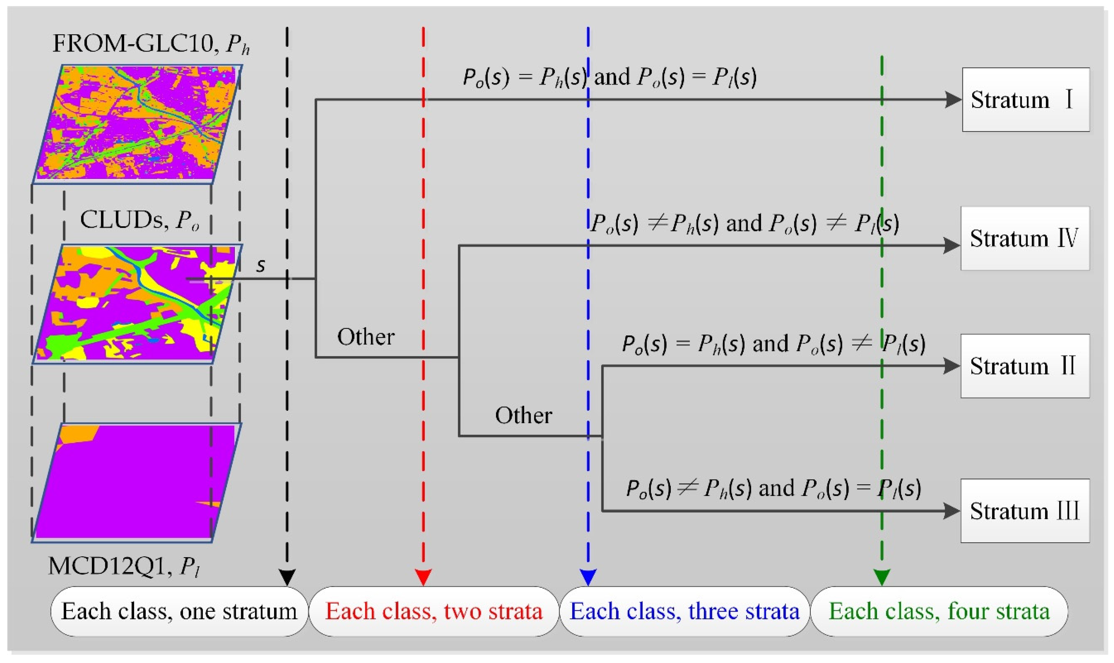
| ID | LULC | CLUDs (30 m) | MCD12Q1 (500 m) | Strata |
|---|---|---|---|---|
| 1 | Cropland | √ | √ | Cropland Ⅰ |
| 2 | √ | × | Cropland Ⅱ | |
| 3 | Woodland | √ | √ | Woodland Ⅰ |
| 4 | √ | × | Woodland Ⅱ | |
| 5 | Grassland | √ | √ | Grassland Ⅰ |
| 6 | √ | × | Grassland Ⅱ | |
| 7 | Water Body | √ | √ | Water Body Ⅰ |
| 8 | √ | × | Water Body Ⅱ | |
| 9 | Built-up Land | √ | √ | Built-up Land Ⅰ |
| 10 | √ | × | Built-up Land Ⅱ | |
| 11 | Unused Land | √ | √ | Unused Land Ⅰ |
| 12 | √ | × | Unused Land Ⅱ |
| Strata | Area Weights (%) | Sample Size | |||||
|---|---|---|---|---|---|---|---|
| Cropland Ⅰ | 12.970 | 18 | 26 | 44 | 85 | 236 | 2129 |
| Cropland Ⅱ | 9.774 | 14 | 19 | 33 | 64 | 178 | 1605 |
| Woodland Ⅰ | 34.425 | 49 | 68 | 116 | 224 | 627 | 5652 |
| Woodland Ⅱ | 11.257 | 16 | 22 | 38 | 73 | 205 | 1848 |
| Grassland Ⅰ | 2.687 | 4 | 5 | 9 | 18 | 49 | 441 |
| Grassland Ⅱ | 5.095 | 7 | 10 | 17 | 33 | 93 | 836 |
| Water Body Ⅰ | 0.647 | 1 | 1 | 2 | 4 | 12 | 106 |
| Water Body Ⅱ | 1.780 | 3 | 4 | 6 | 12 | 32 | 292 |
| Built-up Land Ⅰ | 14.128 | 20 | 28 | 48 | 92 | 257 | 2319 |
| Built-up Land Ⅱ | 6.608 | 9 | 13 | 22 | 43 | 120 | 1085 |
| Unused Land Ⅱ | 0.629 | 1 | 1 | 2 | 4 | 11 | 103 |
| Total | 100 | 142 | 198 | 337 | 652 | 1821 | 16,417 |
| Samples (km × km) | 142 (11 × 11) | 198 (9 × 9) | 337 (7 × 7) | 652 (5 × 5) | 1821 (3 × 3) | 16,417 (1 × 1) | Total |
|---|---|---|---|---|---|---|---|
| OA | 71.278 | 71.783 | 72.926 | 72.123 | 71.127 | 71.110 | 71.083 |
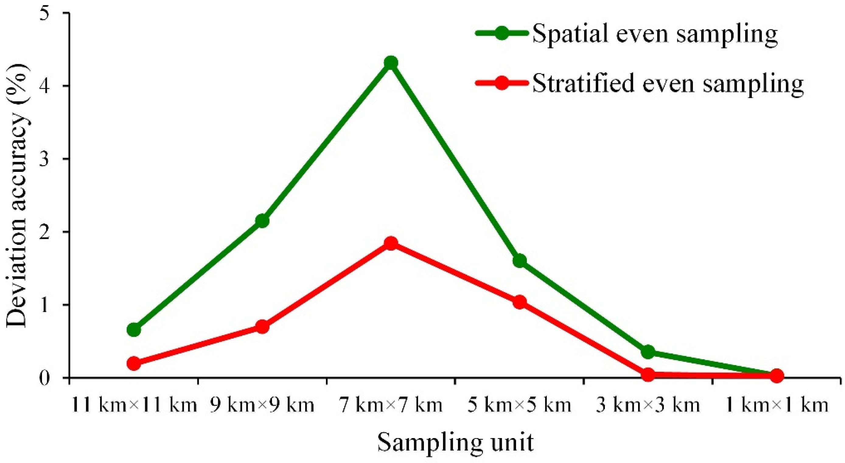
| DA | 0.195 | 0.700 | 1.843 | 1.040 | 0.044 | 0.027 | 0.000 |
| Samples (km × km) | Indices | Cropland | Woodland | Grassland | Water Body | Built-Up Land | Unused Land |
|---|---|---|---|---|---|---|---|
| 142 (11 × 11) | UA | 75.000 | 84.615 | 18.182 | 25.000 | 72.414 | 0.000 |
| PA | 70.588 | 79.710 | 18.182 | 100.000 | 80.769 | 0.000 | |
| 198 (9 × 9) | UA | 71.739 | 78.889 | 26.667 | 20.000 | 80.488 | 0.000 |
| PA | 63.462 | 80.682 | 22.222 | 100.000 | 84.615 | 0.000 | |
| 337 (7 × 7) | UA | 75.325 | 84.416 | 26.923 | 37.500 | 68.571 | 0.000 |
| PA | 68.235 | 83.333 | 28.000 | 60.000 | 73.846 | 0.000 | |
| 652 (5 × 5) | UA | 71.141 | 85.522 | 25.490 | 56.250 | 65.185 | 0.000 |
| PA | 61.272 | 83.007 | 26.531 | 75.000 | 80.734 | 0.000 | |
| 1821 (3 × 3) | UA | 67.633 | 85.577 | 24.648 | 50.000 | 65.252 | 0.000 |
| PA | 61.947 | 81.839 | 25.362 | 75.862 | 76.875 | 0.000 | |
| 16,417 (1 × 1) | UA | 68.595 | 85.637 | 19.367 | 45.067 | 64.803 | 0.000 |
| PA | 61.970 | 81.786 | 20.324 | 71.308 | 78.188 | 0.000 |
| Samples (km × km) | 142 (11 × 11) | 198 (9 × 9) | 337 (7 × 7) | 652 (5 × 5) | 1821 (3 × 3) | 16,417 (1 × 1) | Total |
|---|---|---|---|---|---|---|---|
| OA | 70.423 | 73.232 | 66.766 | 69.479 | 70.730 | 71.115 | 71.083 |
| DA | 0.660 | 2.149 | 4.317 | 1.604 | 0.353 | 0.032 | 0.000 |
| Samples (km × km) | Indices | Cropland | Woodland | Grassland | Water Body | Built-Up Land | Unused Land |
|---|---|---|---|---|---|---|---|
| 142 (11 × 11) | UA | 70.732 | 83.871 | 27.273 | 0.000 | 3.846 | 0.000 |
| PA | 67.442 | 82.540 | 21.429 | 0.000 | 76.190 | 0.000 | |
| 198 (9 × 9) | UA | 63.158 | 91.111 | 11.111 | 57.143 | 76.744 | 0.000 |
| PA | 61.538 | 79.612 | 20.000 | 57.143 | 84.615 | 0.000 | |
| 337 (7 × 7) | UA | 62.667 | 88.194 | 3.846 | 44.444 | 56.098 | 0.000 |
| PA | 58.025 | 78.395 | 5.000 | 80.000 | 68.657 | 0.000 | |
| 652 (5 × 5) | UA | 71.329 | 84.590 | 18.750 | 35.000 | 56.618 | 0.000 |
| PA | 59.302 | 83.226 | 16.071 | 87.500 | 75.490 | 0.000 | |
| 1821 (3 × 3) | UA | 68.127 | 86.617 | 21.818 | 43.590 | 64.810 | 0.000 |
| PA | 60.870 | 79.704 | 26.471 | 68.000 | 80.000 | 0.000 | |
| 16,417 (1 × 1) | UA | 68.595 | 85.612 | 19.367 | 45.067 | 64.803 | 0.000 |
| PA | 61.970 | 81.773 | 20.324 | 71.308 | 78.188 | 0.000 |
Publisher’s Note: MDPI stays neutral with regard to jurisdictional claims in published maps and institutional affiliations. |
© 2022 by the authors. Licensee MDPI, Basel, Switzerland. This article is an open access article distributed under the terms and conditions of the Creative Commons Attribution (CC BY) license (https://creativecommons.org/licenses/by/4.0/).
Share and Cite
Dong, S.; Guo, H.; Chen, Z.; Pan, Y.; Gao, B. Spatial Stratification Method for the Sampling Design of LULC Classification Accuracy Assessment: A Case Study in Beijing, China. Remote Sens. 2022, 14, 865. https://doi.org/10.3390/rs14040865
Dong S, Guo H, Chen Z, Pan Y, Gao B. Spatial Stratification Method for the Sampling Design of LULC Classification Accuracy Assessment: A Case Study in Beijing, China. Remote Sensing. 2022; 14(4):865. https://doi.org/10.3390/rs14040865
Chicago/Turabian StyleDong, Shiwei, Hui Guo, Ziyue Chen, Yuchun Pan, and Bingbo Gao. 2022. "Spatial Stratification Method for the Sampling Design of LULC Classification Accuracy Assessment: A Case Study in Beijing, China" Remote Sensing 14, no. 4: 865. https://doi.org/10.3390/rs14040865
APA StyleDong, S., Guo, H., Chen, Z., Pan, Y., & Gao, B. (2022). Spatial Stratification Method for the Sampling Design of LULC Classification Accuracy Assessment: A Case Study in Beijing, China. Remote Sensing, 14(4), 865. https://doi.org/10.3390/rs14040865