1. Introduction
Precipitation is of great significance in various fields of meteorology and hydrology, such as regional and global water resources, climate change, and numerical weather modeling research [
1,
2,
3]. The application of satellite observations is an vital method to obtain precipitation information [
1,
4,
5,
6,
7]. Compared with radiosonde observations and ground-based remote sensing measurements, satellite remote sensing has the advantages of high temporal sampling frequency, wide spatial coverage, and low cost. Visible light and infrared wave have poor penetration to clouds and precipitation layers. In contrast, the microwave wavelength can be flexibly selected according to practical applications, and the influence of ice clouds and other particles can be ignored or effectively utilized. Therefore, microwave remote sensing has a unique advantage in satellite atmospheric sounding. Since the operation of satellite series Fengyun-3 (FY-3, including FY-3A, 3B, 3C, 3D, 3E), the satellites have obtained rich data for weather, climate, and environmental research [
8].
The Microwave Humidity and Temperature Sounder (MWHTS) onboard FY-3D, as the upgraded instrument of the Microwave Humidity Sounder (MWHS), has included the detection frequencies of 89 GHz and 118.75 GHz in addition to the original channels, making it the first instrument on a polar-orbiting meteorological satellite in the world to carry out atmospheric observations with a 118.75 GHz radiometer. MWHTS is generally used to retrieve atmospheric temperature and water vapor in order to estimate precipitation and forecast typhoon paths [
9,
10]. In addition, MWHTS observations further strengthen and increase the resiliency of the microwave branch of the observing system used for numerical weather prediction (NWP) [
11].
Precipitation retrieval methods can be roughly divided into three categories: statistical methods (e.g., [
12,
13]), physical methods (e.g., [
14,
15,
16]), and combined physical–statistical methods (e.g., [
17]). Compared with physical inversion systems, statistical methods can not only avoid background field information from the atmospheric radiative transfer equation but also have the advantages of low complexity, high calculation efficiency, and fewer variables. In a statistical algorithm for precipitation, Cui et al. [
18] used the satellite data of MWHS/FY-3A during three severe tropical storms to estimate the precipitation by multiple linear regression method. He et al. [
19] developed a passive sub-millimeter atmospheric profile and precipitation retrievals algorithm for MWHTS onboard the FY-3C satellite. Researchers also found that the MWHTS channels at 118.75 GHz and 183.31 GHz are helpful in detecting precipitation [
20]. On this basis, Li et al. [
21] proposed an improved algorithm for precipitation retrievals based on brightness temperature (TB) data observed by MWHTS/FY-3C using linear regression and a neural network method. In addition, Chen et al. [
22] evaluated the impacts of emissivity atlas and the dynamic emissivity for assimilation. The results indicate that the use of the dynamic emissivity retrieved from the 89 GHz channel of MWHTS/FY-3C apparently increases the amount of assimilated data and improves the initial fields and the 24 h forecasts of precipitation distribution and intensity.
In recent years, machine learning algorithms have gained increasing interest in precipitation research (e.g., [
7,
23,
24]). Nevertheless, studies on comparing and quantifying the performance of different machine learning models for satellite precipitation retrievals are rare to none. In addition, optimization processes of some key hyperparameters in machine learning models (i.e., parameters that need to be predefined) have not been thoroughly investigated, which can greatly affect the model performance. In fact, most studies have only utilized TB at different channels as inputs [
21], which may not be sufficient to represent precipitation characteristics, resulting in higher inversion errors.
Therefore, there are three main purposes of this study: (1) In addition to using TB at different MWHTS channels, three linear TB combinations are proposed as inputs for precipitation retrievals, which can better characterize precipitation at different intensities and further improve the retrieval accuracy; (2) Using grid search and cross-validation methods to explore the optimal hyperparameters of machine models, this paper compares the performance and explores the feasibility and rationality of four machine learning models (RFR, SVM, MLP, and GBRT) for precipitation retrieval; (3) This article also quantifies the retrieval advantages with the addition of linear combinations as inputs and verifies the robustness of the ensemble learning models.
2. Dataset and Input Selection
2.1. MWHTS Observations and Its Channels
When FY-3D operates in polar orbit, the MWHTS observations can be obtained every 102 min. Firstly, the original observation data on the satellite need to be processed by quality inspection, identification, and control. Then, the data are calibrated successively by two-point calibration, system nonlinear correction, and antenna pattern correction. Finally, level-1 TB data are obtained. Detailed parameters are shown in
Table 1.
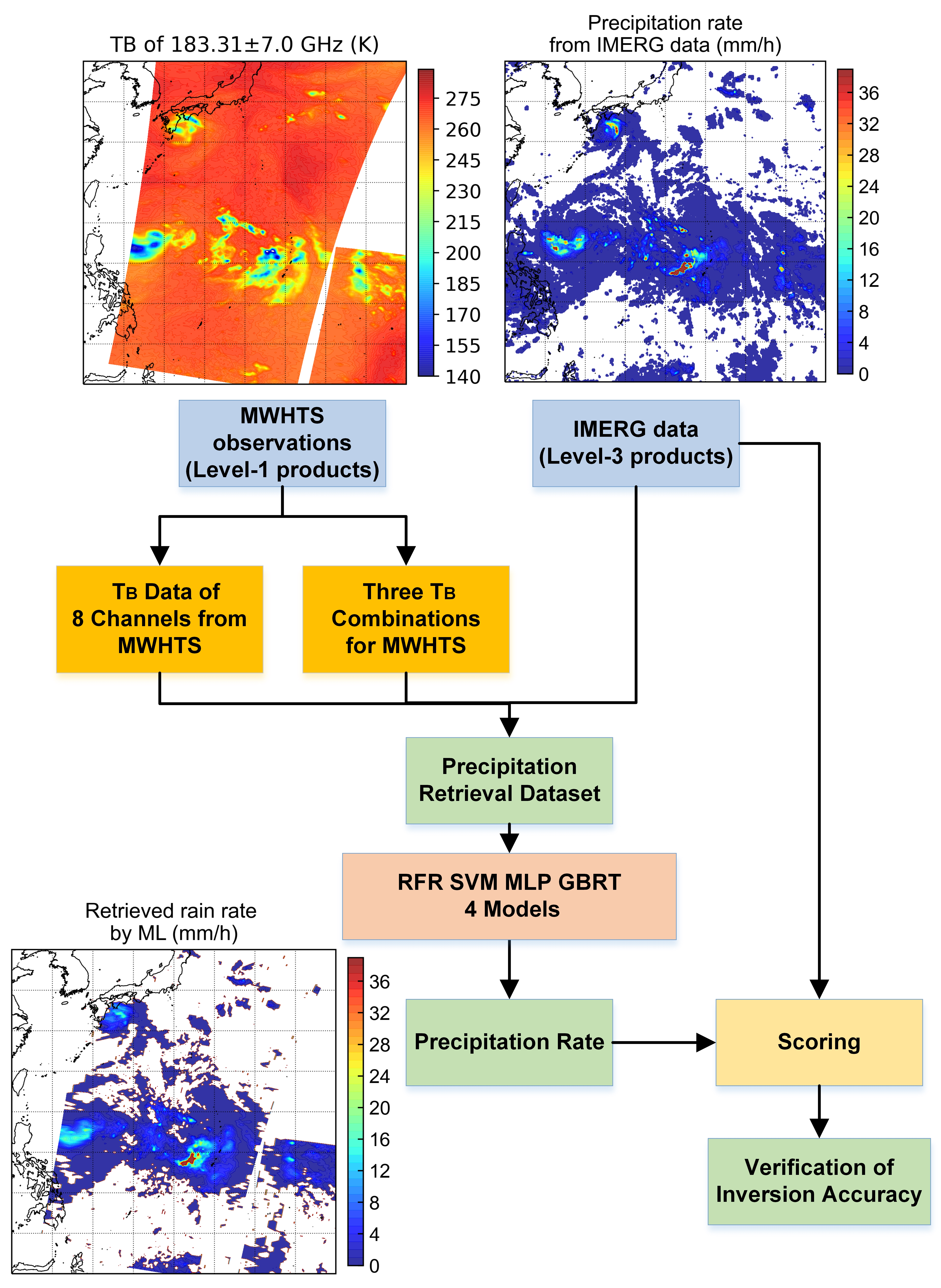
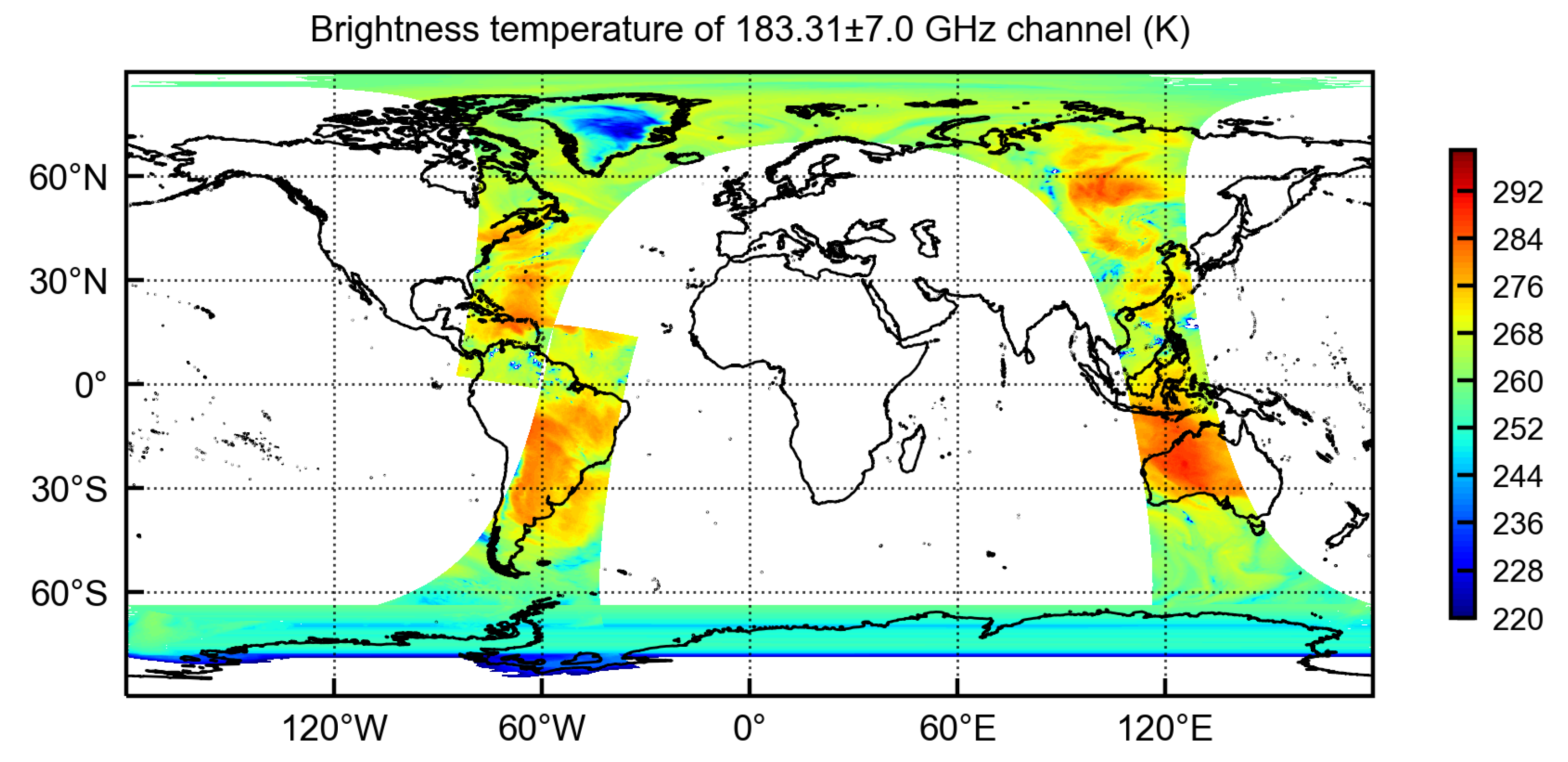
Figure 1 shows the global TB data observed by FY-3D MWHTS of 183.31 ± 7.0 GHz channel around the Earth polar orbit from 04:33 to 06:15 UTC on August 05 2019, from which we can see the global TB data distribution information of land and ocean observed by MWHTS.
2.2. IMERG Data
The IMERG-Late Run (Version 6) used in this paper provides half-hourly precipitation estimates on a 0.1
× 0.1
grid resolution by the Integrated Multi-satellite Retrievals for GPM (IMERG). IMERG data is intended to intercalibrate, merge, and interpolate satellite microwave precipitation estimates, together with microwave-calibrated infrared (IR) satellite estimates and precipitation gauge analyses [
25]. The precipitation estimates from various satellite passive microwave (PMW) sensors comprising the GPM constellation are computed using the Goddard Profiling Algorithm [
5], then gridded, intercalibrated to the GPM Combined Ku Radar–Radiometer Algorithm (CORRA) product and merged into half-hourly 0.1
× 0.1
fields. The intercalibrated merged PMW estimates are then input to both the Climate Prediction Center (CPC) Morphing-Kalman Filter (CMORPH-KF) Lagrangian time interpolation scheme [
26] and the precipitation estimation from remotely sensed information [
27]. The CMORPH-KF morphing uses the PMW and IR estimates to create half-hourly estimates. After obtaining the satellite observations, IMERG-Late Run is computed about 14 h after observation time using both forward and backward morphing.
Figure 2 shows the IMERG data (mm/h) from 03:30 to 04:30 UTC on 5 August 2019.
2.3. Temporal and Spatial Matching and Preprocessing
In this paper, MWHTS observations (level-1 products) and IMERG data (level-3 products) collected from 1 July 2019 to 31 August 2019 are used for precipitation retrieval model training and testing. The matching domain covers (0N–40N, 120E–140E). Since there may be some unreasonable data, such as lack of measurement or precipitation pixels of low quality scores, the following steps are executed to ensure the data credibility:
For MWHTS observations, the missing data can be determined according to channel data integrity quality, and the data quality can be determined by the Earth observations quality score field. The score ranges from 0 to 100. In this paper, only the data with score of 100 (data with the best quality) are selected. For IMERG, product quality can be determined according to the precipitation quality index field. Simultaneously, the data rationality of the temporal and spatial matching will also directly affect the accuracy of precipitation inversion. Given the time interval of half an hour for IMERG data, temporal matching resolution is 30 min (the time difference between the two observation samples is less than half an hour). Since IMERG data are global grid data with a resolution of 0.1× 0.1 and the nadir point size of MWHTS is 16 km × 16 km for 183.31 GHz, spatial matching resolution is set as 0.15× 0.15.
Compared with ocean, the natural background of land is more complex. Therefore, the matched data are divided into two categories (hereafter referred to as ocean and land data) according to the region of the matched data, to establish inversion models to improve the accuracy of precipitation retrieval for both ocean and land regions. After completing the matching steps, there are 55,520 matched data samples over ocean and 39,934 samples over land.
2.4. Input Selection
In contrast to the method in which the TB at each channel is directly taken as the input for the inversion, this article first analyzes the correlation coefficients of the TB at 15 channels observed by MWHTS (
Figure 3). It can be inferred from
Figure 3 that the correlation coefficients of TB at 15 channels over ocean and land region are generally consistent. Compared with continental precipitation, the number of smaller raindrops in ocean precipitation is higher, and the number of larger raindrops is lower [
28,
29]. In the weather scenarios with high water vapor content, the scattering effect of raindrops on microwave is stronger, so the TB is more sensitive to raindrops. The correlation between the three channels at 118.75 GHz (118.75 ± 2.5, 118.75 ± 3.0, and 118.75 ± 5.0 GHz) is relatively high, and a similar phenomenon occurs for five channels at 183.31 GHz. Li et al. simulated the TB of MWHTS under water cloud weather conditions, and the results indicated that three channels set at 118.75 GHz are more sensitive to the change of cloud water content and equivalent particle radius than other 118.75 channels [
21]. Five channels set at 183.31 GHz also show the same result. This is consistent with the TB correlation coefficient of each channel in
Figure 3, which further illustrates the ability of these channels to detect raindrops and clouds in the atmosphere.
In order to avoid data redundancy and save the training time, if the correlation coefficient between a channel and other channels is greater than 0.9, the data of this channel will not be selected as the input. Therefore, this paper firstly selected TB set at 89.0 GHz, 118.75 ± 0.08 GHz, 118.75 ± 0.2 GHz, 118.75 ± 0.8 GHz, 118.75 ± 1.1 GHz, 118.75 ± 2.5 GHz, 183.31 ± 1.0 GHz, and 183.31 ± 3.0 GHz detection frequencies as inputs over both ocean and land regions.
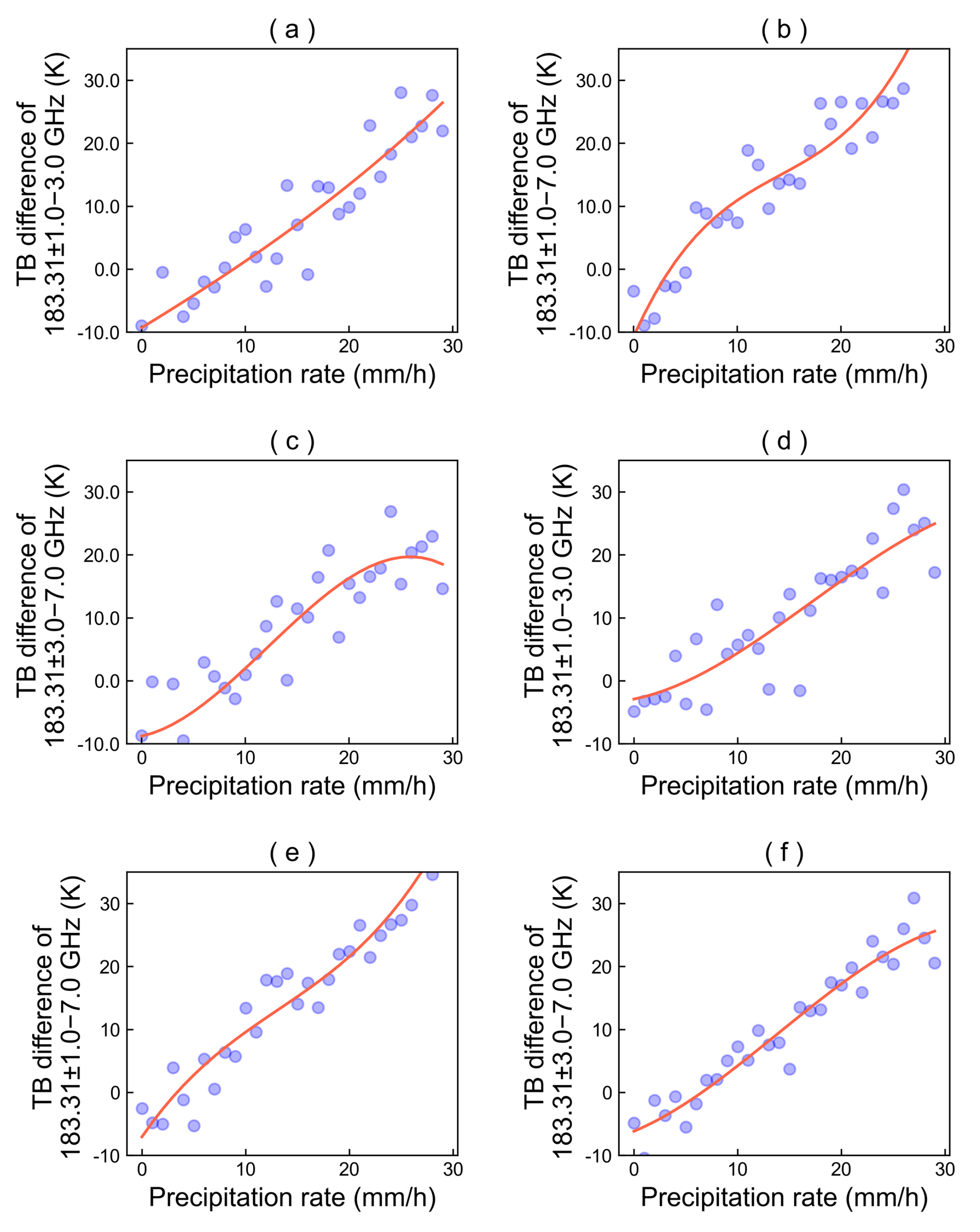
A crucial step for precipitation inversion is to construct the proper model and determine inputs of the model. To this end, different TB-derived variables were considered. In addition to applying measured TB at different MWHTS channels, their differences and linear combinations are taken into account to further resolve the correlation with rain rate. In particular, three linear TB differences, i.e., 183.31 ± 1.0–183.31 ± 3.0 GHz, 183.31 ± 1.0–183.31 ± 7.0 GHz, and 183.31 ± 3.0–183.31 ± 7.0 GHz are also selected as inputs to retrieve rain rate. Three channels (183.31 ± 1.0 GHz,183.31 ± 3.0 GHz, and 183.31 ± 7.0 GHz) have different weight heights, and channels away from 183.31 GHz have lower weight peak heights (
Table 1). In the case of light rain, the TB observed by 183.31 ± 1.0 GHz is lower than that of the other two channels. With the increase of rainfall rate, the channel away from 183.31 GHz is more affected by the scattering of ice particles from the lower layer of the cloud. As a result, TB further decreases and the TB difference further increases. The results show that linear combinations between channels can be well fitted by cubic polynomial, which can better characterize precipitation of different intensities and further improve the retrieval performance. The specific fitting equations and linear combinations scatter plots are shown in
Table 2 and
Figure 4 (in
Table 2, R refers to the rainfall rate, and C refers to TB differences calculated by fitting equations. For example, C in the second row of
Table 2 represents TB differences of 183.31 ± 1.0–183.31 ± 3.0 GHz). Compared with classical approaches such as principal components to combining channels, the contribution of channel difference combinations for precipitation inversion is clearly displayed, which makes the physical interpretability of the statistical inversion method stronger. As can be seen from
Figure 4, the fitting effect of these three linear combinations is good. In addition, IMERG data are basically consistent with the precipitation distribution intensity and other details observed by the TB difference at MWHTS channels (
Figure 5). Therefore, from a qualitative point of view, it has certain rationality and feasibility to apply three linear combinations to retrieve precipitation. and it can be intuitively predicted that adding these linear combinations as inputs will improve the retrieval accuracy. The specific results will be introduced in detail in the following sections.
3. Methodologies
3.1. Retrieval Framework
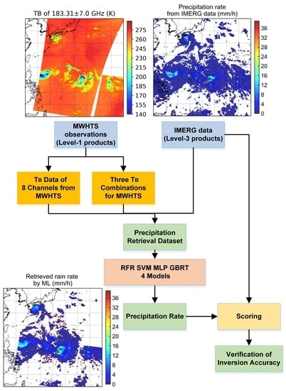
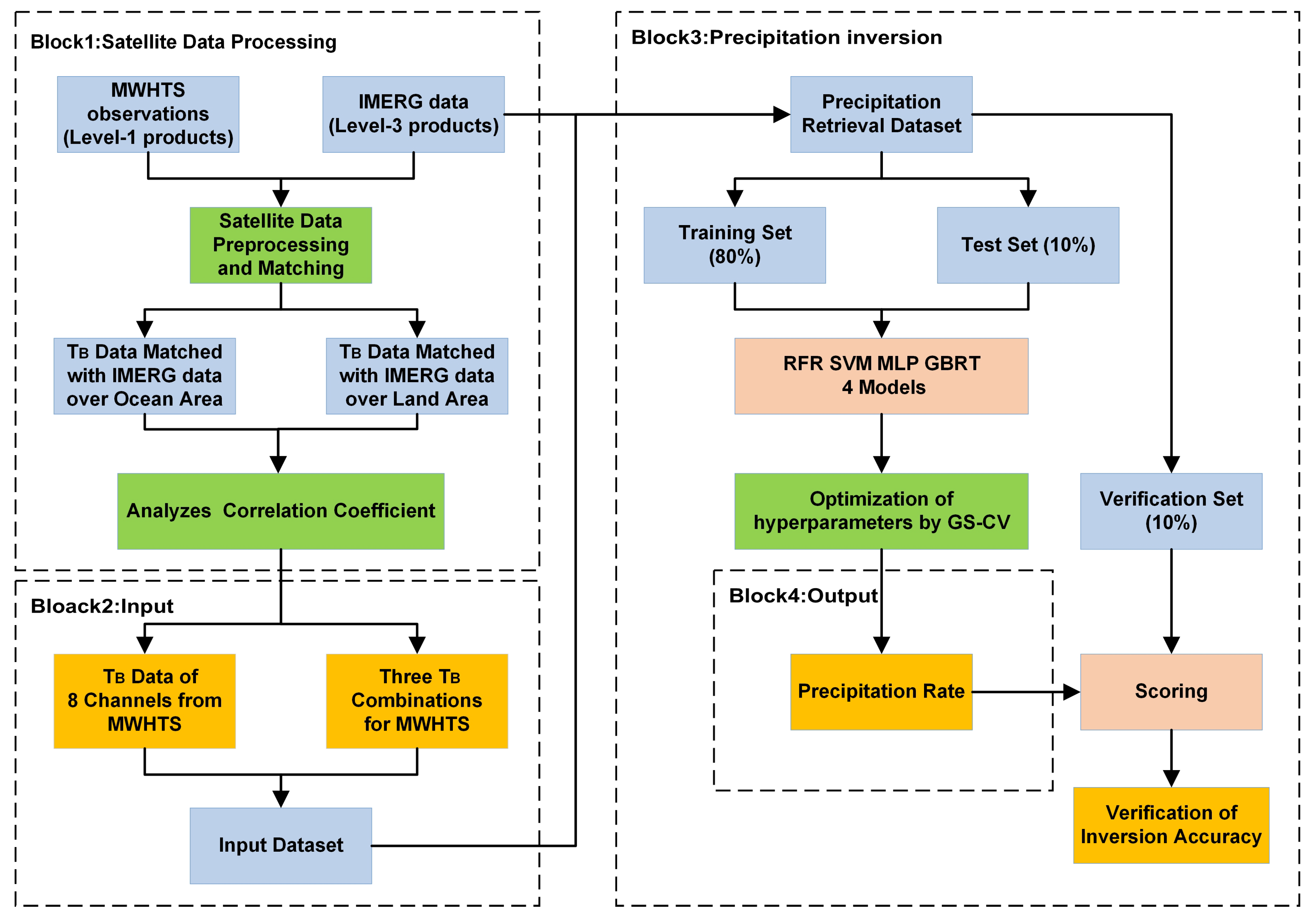
Figure 6 shows the overall steps of this research. Firstly, the MWHTS observations and IMERG data are preprocessed to control the data quality, then TB data are matched with IMERG data over ocean and land region and the correlation of TB data of each channel is analyzed to remove the redundant channel data (see block 1 in
Figure 6). In addition to selecting TB in the different MWHTS channels, three linear TB combinations (183.31 ± 1.0–183.31 ± 3.0 GHz, 183.31 ± 1.0–183.31 ± 7.0 GHz, and 183.31 ± 3.0–183.31 ± 7.0 GHz) are also proposed as inputs (see block 2 in
Figure 6). The output of the model is precipitation rate (see block 4 in
Figure 6). The precision retrieval database consists of inputs and corresponding IMERG data. Each channel data was normalized before training the model.
For an accurate performance evaluation, a proper data splitting into a training set, a test set, and a verification set is required. The training set is the data sample for model fitting. To evaluate our model performance, an independent test set is applied to tune the hyperparameters of the models using grid search and cross-validation (GS-CV) methods, monitor whether the model has been fitted, and evaluate the model performance. Selecting the training model that performs the best on the test set introduces the risk of overfitting, so an independent verification set is chosen to evaluate the generalization ability of the trained models. Specifically, the training set accounts for 80%, test set accounts for 10%, and verification set accounts for 10%, with 55,520 totally matched data points over ocean and 39,934 matched data points over land.
3.2. Machine Learning Models
Based on the matched TB data, this article constructs four machine learning models: random forest regressor (RFR) [
30], support vector machine (SVM), multilayer perceptron (MLP), and gradient boosting regression tree (GBRT).
Random forest regression (RFR) is a bagging algorithm. The general idea of RFR is training several weak models to form a strong model, as the performance of a strong model is much better than that of a single weak model. In the training stage, RFR adopts bootstrap sampling to collect different sub-datasets from the input dataset and averages the prediction results of multiple decision trees to obtain the final output. The number of trees, , is an important parameter. As a machine learning method, RFR has good processing abilities for high-dimensional data and can process huge amounts of data. Simultaneously, the RFR model has strong generalization ability and robustness.
The support vector machine (SVM) can be used for classification or regression. The basic model is the linear classifier with the largest interval defined in the feature space. SVM also includes kernel techniques, which make them essentially nonlinear classifiers. The basic idea is to make the input space correspond to a feature space through nonlinear transformation so that the hypersurface model in the input space corresponds to the hyperplane model in the feature space. The learning strategy of a support vector machine is to maximize the interval, which is equivalent to a convex quadratic programming problem. SVM has been applied in many fields, such as temperature and humidity profile retrievals [
31,
32]. The key hyperparameter optimization of support vector machines mainly includes the Gaussian kernel parameter (
) and penalty factor (
C).
The multilayer perceptron (MLP) is a model that imitates the structure and function of biological neural networks, and adopts an error back-propagation algorithm and has strong dynamic processing ability. It can realize highly nonlinear mapping without knowing the relationship between the inputs and outputs. Because of its simple structure and strong plasticity, it has been widely used in many fields. MLP is fully connected between layers, and there is no coupling between nodes in the same layer [
21]. Data are transmitted from the input layer to the hidden layer, and the connection weight of the network is corrected from the output layer. In the error signal back-propagation phase, the weight is adjusted layer-by-layer. As the learning process continues, the error gradually decreases. However, it is easy for it to fall into local optimal solutions and it is sensitive to input datasets. The hyperparameters of the MLP mainly include the activation functions and the number of hidden neurons.
Gradient boosting regressor tree (GBRT) is an iterative decision tree algorithm which realizes precipitation inversion using cumulative output of many previous models and continuously reducing the residual generated in the training process [
33]. GBRT generates a weak model through multiple rounds of iterations and the loss function decreases along the gradient direction. In this way, the loss function is reduced continuously and the convergence can reach the optimal solution. The main parameter of the model is the number of trees:
.
3.3. Model Evaluation Criteria
For precipitation retrieval, the mean squared error (MSE), mean absolute error (MAE), and R-square (R
2) are proposed as the evaluation criteria of the model. MSE (mm/h) and MAE (mm/h) measure the degree of deviation between the truth and predicted value. Obviously, lower MSE and MAE values indicate that a model has better performance. The value range of R
is [0,1], and the closer the value is to 1, the stronger the explanatory power of the TB in the regression equation is to rain rate. The equations used to calculate MSE, MAE, and R
2 can be expressed as follows (
Table 3). Where
is the predicted value of the
sample;
is the corresponding truth value;
n is the total number of samples.
3.4. Parameter Tuning
In a machine learning model, inappropriate hyperparameters will trigger underfitting or overfitting issues. In this case, the values of hyperparameters are crucial. However, manual selection for hyperparameters will consume an inordinate amount of time. To this end, the GS-CV method [
34] is applied to optimize the hyperparameter which can be divided into two parts: grid search and cross-validation.
For grid search, the machine learning model iterates through all candidate combinations of hyperparameters, tries every possibility, and selects the best hyperparameters as the final result. This is actually a process of training and comparison. In this paper, MAE is used to evaluate model performance. Grid search ensures that parameters with high precision can be found within the specified parameter range. For cross-validation, cross-validation is used, which can effectively reduce overfitting phenomenon and improve the generalization ability of the model. Specifically, the matched data except verification set are divided into k copies (k = 9 in this paper), the copy is taken as the test set, and the remaining copies are used as the training set for the cross-validation. This process is repeated a total of k times, and the average of performance indicators of the regression model is returned. When the hyperparameters are optimized by the grid search, cross-validation is used to evaluate each group of hyperparameters. Finally, the optimal combination of hyperparameters is selected to establish the model.
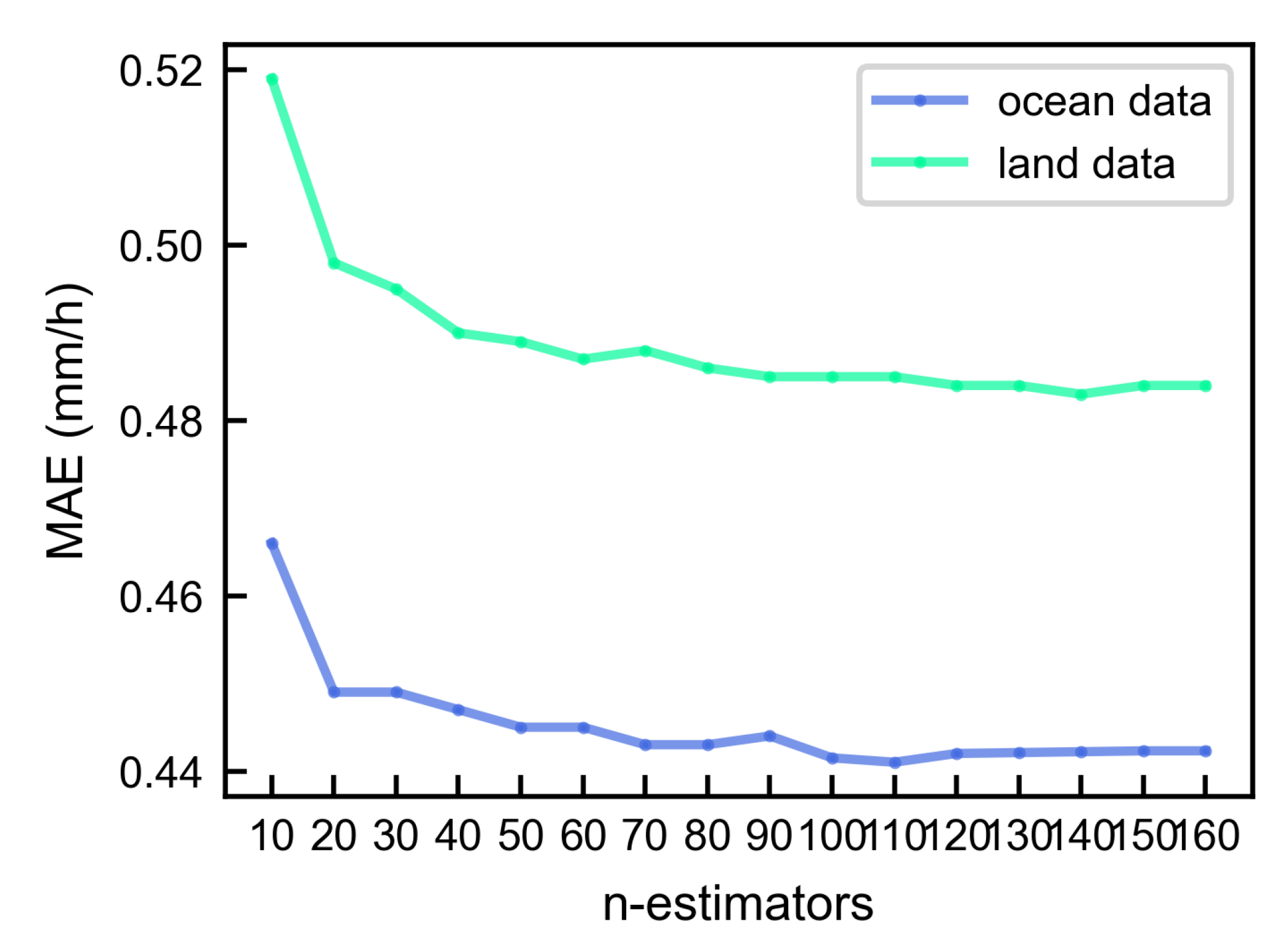
For the RFR model, the value of
to be optimized is from 10 to 160 and bootstrapping is used for the sampling. MAE values under different
are shown in
Figure 7. When the n-estimators are 110 and 140, the MAE values based on ocean and land data are the lowest, respectively.
For the SVM regression model, MAE values of the model obtained under different
C and
are shown in
Figure 8. Compared with the model based on ocean data, the accuracy based on land data changes little with different parameters. If the
C value is increased (
) blindly (greater than one), the improvement of retrieval accuracy is very limited, which will consume unnecessary time. In view of this situation, for both ocean and land models,
and
are selected.
The number of hidden layer neurons of the MLP model is optimized from 20 to 150, and the activation function is selected from
,
, and
(
Figure 9). The
is set to 200,
is 0.0001, and
optimizer is selected to continuously reduce losses. When activation function is
and the number of neurons in the hidden layer is 40, the ocean model is optimal, and are
and 60 respectively, for the land model results.
For the GBRT model, whether based on ocean or land data, MAE value almost does not decrease when
reaches 180 (
Figure 10). The model is considered to be optimal approximately when
is 180. The learning rate of the model is set to 0.01.
With GS-CV methods, hyperparameters of machine learning models were optimized, as shown in
Table 4.
4. Results and Analysis
In this study, TB and TB combinations are proposed as inputs. However, the limitations of linear combinations lie in the interpretability of potential physical processes. This leads to the question of whether the machine learning model with linear combinations as inputs is better than the model without them. To this end, this paper explores the contribution of the linear combinations for precipitation retrieval. Specifically, for each machine learning model, (1) only TB of eight channels; (2) TB of eight channels and linear combination (183.31 ± 1.0–183.31 ± 3.0 GHz); (3) TB of eight channels and linear combination (183.31 ± 1.0–183.31 ± 7.0 GHz); (4) TB of eight channels and linear combination (183.31 ± 3.0–183.31 ± 7.0 GHz); (5) TB of eight channels and three linear combinations are used as inputs. This will allow the advantages of linear combination to be quantified individually and compared with performance of their combined inversion. Hyperparameters of four machine learning models for retrieval precipitation were determined by GS-CV methods to compare and assess the performance of models. Final results using the verification set are shown in
Figure 11 (with inputs (5)) and
Table 5. In the case of adding three combinations, it can be inferred from
Figure 11 and
Table 5 that applying four machine learning models to retrieved precipitation is feasible and rational. For regression scores based on ocean verification data, the RFR model has the best performance, with MSE, MAE, and R
2 of 1.75 mm/h, 0.44 mm/h, and 0.80, respectively, and the retrieval accuracy of GBRT model is almost as good as RFR, with MSE, MAE, and R
2 of 1.80 mm/h, 0.45 mm/h, and 0.78, respectively, followed by the MLP model. The performance of precipitation inversion based on SVM is not outstanding.
In addition, retrieval results indicate the retrieval advantages by adding linear combination as inputs. Regardless of the model, linear combination (183.31 ± 1.0–183.31 ± 3.0 GHz) will slightly improve the model performance. Compared with using only TB of eight channels as inputs, the R2 of RFR, SVM, MLP, and GBRT increased by 0.02, 0.01, 0.04, and 0.02, respectively, after adding combination (183.31 ± 1.0–183.31 ± 3.0 GHz). Simultaneously, two other linear combinations can significantly outperform linear combination (183.31 ± 1.0–183.31 ± 3.0 GHz), almost reaching the accuracy of adding them all, especially for 183.31 ± 3.0–183.31 ± 7.0 GHz. For the precipitation inversion based on land data, the background and natural factors are more complex. Simultaneously, there is higher water vapor content in the atmosphere above the ocean surface, and the scattering effect of raindrops in ocean precipitation on microwave is stronger, so the TB is more sensitive to raindrops. Therefore, the retrieval accuracy is lower than that of corresponding results based on ocean data. The improvement of retrieval performance by each linear combination is consistent with that based on ocean data. Adding linear combination (183.31 ± 1.0–183.31 ± 3.0 GHz) as inputs will slightly enhance the performance, while adding two other combinations greatly improves retrieval accuracy, almost as accurate as adding them all.
It can be inferred that no matter which kind of machine learning model is applied based on ocean or land data, retrieval accuracy is improved with linear combinations as additional inputs, indicating that linear combinations can enhance the extraction performance of complex physical relationship between the TB and precipitation rate. This further confirms the contribution of three linear combinations to precipitation inversion.
Simultaneously, this paper analyzes the results from the perspective of the different rain rates and temporal matching difference between MWHTS and IMERG data (
Table 6). The results show that the performance changes of the four machine models are basically the same under different rain rates and temporal matching difference. Performances are better among the various evaluation criteria for heavy rain versus light. Compared with heavy rain, temporal matching difference of light rain has little effect for retrieval performance. As the temporal matching resolution is 30 min, the real rainfall rate corresponding to the TB cannot be accurately matched for some data pixels. High rainfall rates would tend to be associated with short duration event, resulting in a large gap between the matched and real rainfall rate, which leads to the decline of retrieval performance.
For an additional qualitative evaluation, this paper takes a precipitation from 13:30 to 14:30 UTC on August 05 2019 over the Northwest Pacific region as the case, performs the spatial maps of retrieval results using models, and compares them to MWHTS observations and IMERG data (
Figure 12). The location, distribution, and structure information (
Figure 12c–f) retrieved by machine learning models are clearly displayed. Simultaneously, retrieved precipitation spatial distribution is greatly consistent with IMERG data. Therefore, from a qualitative point of view, four machine learning models are feasible and scientific.
5. Discussion
Both RFR and GBRT models belong to ensemble learning algorithms (including bagging and boosting methods). They combine multiple weakly supervised models to obtain a better model. The fundamental idea of ensemble learning is that even if one weak supervised model obtains relatively inaccurate prediction, other weak models can correct the error to a certain extent. Specifically, the RFR model is characterized by the bagging method. That is, bootstrap sampling is applied to randomly select samples from the training set for N times. In that case, N weak supervised models are trained independently, and final output is obtained through ensemble strategy. It is worth noting that N weak models are independent of each other and are trained in parallel. Simultaneously, because the training set changes with each sampling, the results of N weak models are different, which shows that the bagging method has strong generalization ability and plays a significant role in reducing model variance. The GBRT model adopts gradient boosting algorithm based on the boosting method. In the function space, the loss function decreases along the gradient direction, and model performance is improved by reducing the deviation. In the training process, a weak supervision model is firstly initialized to obtain the predicted value and loss, and then the subsequent model learns according to the previous model loss. Each step of iteration can make up for the shortcomings of the previous model. Finally, the predicted value of the model is the cumulative output of many previous models. Therefore, whether based on ocean data or land data, the RFR and GBRT model have strong generalization abilities and performance.
The above analysis illustrates that machine learning is a powerful tool for data analysis and extracting the complex relationships between variables. In addition, this paper incorporates three TB combinations as inputs, which can better characterize precipitation at different intensities and further improves the retrieval accuracy. Nevertheless, the robustness and antinoise ability of the four machine learning methods need to be further tested. To this end, this paper adds Gaussian distribution noises with variance of 0.4, 0.8, 1.2, 1.6, and 2 on the TB (
Figure 13).
From
Figure 13, it can be inferred that RFR and GBRT models still have the best retrieval performance under Gaussian noise condition, which reflects the strong robustness and antinoise performance of the ensemble learning algorithm. Compared with the results based on ocean data, the models based on land data are more sensitive to noise due to the more complex background, especially for SVM and MLP models. When the variance of noise changes from 0 to 2, the MSE of the MLP model increases from 1.96 mm/h to 4.13 mm/h and the MSE of the SVM model changes from 2.72 mm/h to 4.65 mm/h. Therefore, models based on ocean area have stronger ability to explain and fit precipitation, to a certain extent.
6. Conclusions
Based on MWHTS observations, four machine learning models (RFR, SVM, MLP, and GBRT) are applied for precipitation retrieval. This paper determines the optimal hyperparameters of the machine models using grid search and cross-validation methods. Simultaneously, this research adds TB combinations as additional inputs, which can better characterize precipitation of different intensities. The encouraging results show that retrieval accuracy is significantly improved with linear combinations, especially for 183.31 ± 3.0–183.31 ± 7.0 GHz and 183.31 ± 1.0–183.31 ± 7.0 GHz. In addition, this paper analyzes the retrieval results from the perspective of the different rain rates and temporal matching difference between MWHTS and IMERG data. The generalization capability and robustness of each machine learning model are also analyzed. It can be inferred that the RFR model and the GBRT model still maintain the best retrieval accuracy under different Gaussian noise conditions, indicating the strong robustness and antinoise performance of ensemble learning models for precipitation retrieval.
With the successful launch of satellite series FY-3, MWHTS onboard FY-3 can be considered as supplementary instruments for multi-sensor products in the future and make further valuable contributions to the global precipitation observation system. In addition to that, deep learning techniques should be considered in future development of satellite precipitation retrieval algorithms. Simultaneously, machine learning models in this paper rely only on the passive microwave radiometer to retrieve precipitation; future work can focus on the introduction of radar data and other multisource data for joint retrieval.
Author Contributions
Conceptualization, K.L. and J.H.; methodology, K.L.; software, K.L.; validation, K.L., J.H. and H.C.; formal analysis, J.H.; investigation, K.L., J.H. and H.C.; resources, J.H.; data curation, K.L.; writing—original draft preparation, K.L.; writing—review and editing, H.C. and J.H.; visualization, K.L.; supervision, H.C. and J.H.; project administration, J.H. and H.C.; funding acquisition, J.H. and H.C. All authors have read and agreed to the published version of the manuscript.
Funding
This work was funded in part by the National Key R&D Program of China (2018YFB0504900, 2018YFB0504902) and in part by the Youth Promotion Association of the Chinese Academy of Sciences (2016136). The work of Haonan Chen was funded by the National Oceanic and Atmospheric Administration (NOAA) Joint Polar Satellite System (JPSS) Proving Ground and Risk Reduction program.
Institutional Review Board Statement
Not applicable.
Informed Consent Statement
Not applicable.
Data Availability Statement
Acknowledgments
We appreciate constructive comments from anonymous reviewers that helped us improve our manuscripts.
Conflicts of Interest
The authors declare no conflict of interest.
References
- Hou, A.Y.; Kakar, R.K.; Neeck, S.; Azarbarzin, A.A.; Kummerow, C.D.; Kojima, M.; Oki, R.; Nakamura, K.; Iguchi, T. The Global Precipitation Measurement Mission. Bull. Am. Meteorol. Soc. 2014, 95, 701–722. [Google Scholar] [CrossRef]
- Chen, H.; Chandrasekar, V. The quantitative precipitation estimation system for Dallas–Fort Worth (DFW) urban remote sensing network. J. Hydrol. 2015, 531, 259–271. [Google Scholar] [CrossRef]
- Ma, Y.; Chandrasekar, V.; Chen, H.; Cifelli, R. Quantifying the Potential of AQPI Gap-Filling Radar Network for Streamflow Simulation through a WRF-Hydro Experiment. J. Hydrometeorol. 2021, 22, 1869–1882. [Google Scholar] [CrossRef]
- Kummerow, C.; Barnes, W.; Kozu, T.; Shiue, J.; Simpson, J. The Tropical Rainfall Measuring Mission (TRMM) Sensor Package. J. Atmos. Ocean. Technol. 1998, 15, 809–817. [Google Scholar] [CrossRef]
- Kummerow, C.; Hong, Y.; Olson, W.S.; Yang, S.; Adler, R.F.; McCollum, J.; Ferraro, R.; Petty, G.; Shin, D.B.; Wilheit, T.T. The Evolution of the Goddard Profiling Algorithm (GPROF) for Rainfall Estimation from Passive Microwave Sensors. J. Appl. Meteorol. 2001, 40, 1801–1820. [Google Scholar] [CrossRef]
- Joyce, R.J.; Janowiak, J.E.; Arkin, P.A.; Xie, P. CMORPH: A Method that Produces Global Precipitation Estimates from Passive Microwave and Infrared Data at High Spatial and Temporal Resolution. J. Hydrometeorol. 2004, 5, 487–503. [Google Scholar] [CrossRef]
- Chen, H.; Sun, L.; Cifelli, R.; Xie, P. Deep Learning for Bias Correction of Satellite Retrievals of Orographic Precipitation. IEEE Trans. Geosci. Remote Sens. 2021, 60, 4104611. [Google Scholar] [CrossRef]
- Dong, C.; Yang, J.; Zhang, W.; Yang, Z.; Lu, N.; Shi, J.; Zhang, P.; Liu, Y.; Cai, B. An overview of a new Chinese weather satellite FY-3A. Bull. Am. Meteorol. Soc. 2009, 90, 1531–1544. [Google Scholar] [CrossRef]
- He, J.; Zhang, S.; Li, N. Precipitation Retrievals in typhoon domain combining of FY3C MWHTS Observations and WRF Predicted Models. In Proceedings of the IOP Conference Series: Earth and Environmental Science, Shanghai, China, 19–22 October 2017; IOP Publishing: Bristol, UK, 2017; Volume 57, p. 012049. [Google Scholar]
- He, J.; Chen, H. Atmospheric Retrievals and Assessment for Microwave Observations from Chinese FY-3C Satellite during Hurricane Matthew. Remote Sens. 2019, 11, 896. [Google Scholar] [CrossRef]
- Carminati, F.; Atkinson, N.; Candy, B.; Lu, Q. Insights into the Microwave Instruments Onboard the Fengyun 3D Satellite: Data Quality and Assimilation in the Met Office NWP System. Adv. Atmos. Sci. 2021, 38, 1379–1396. [Google Scholar] [CrossRef]
- Berg, W.; Olson, W.; Ferraro, R.; Goodman, S.J.; LaFontaine, F.J. An assessment of the first-and second-generation navy operational precipitation retrieval algorithms. J. Atmos. Sci. 1998, 55, 1558–1575. [Google Scholar] [CrossRef]
- Ferraro, R.R.; Marks, G.F. The development of SSM/I rain-rate retrieval algorithms using ground-based radar measurements. J. Atmos. Ocean. Technol. 1995, 12, 755–770. [Google Scholar] [CrossRef]
- Shibata, A.; Imaoka, K.; Koike, T. AMSR/AMSR-E level 2 and 3 algorithm developments and data validation plans of NASDA. IEEE Trans. Geosci. Remote Sens. 2003, 41, 195–203. [Google Scholar] [CrossRef]
- Wentz, F.J.; Spencer, R.W. SSM/I rain retrievals within a unified all-weather ocean algorithm. J. Atmos. Sci. 1998, 55, 1613–1627. [Google Scholar] [CrossRef]
- Liu, S.; Grassotti, C.; Liu, Q.; Lee, Y.-K.; Honeyager, R.; Zhou, Y.; Fang, M. The NOAA Microwave Integrated Retrieval System (MiRS): Validation of Precipitation From Multiple Polar-Orbiting Satellites. IEEE J. Sel. Top. Appl. Earth Obs. Remote Sens. 2020, 13, 3019–3031. [Google Scholar] [CrossRef]
- Boukabara, S.A.; Garrett, K.; Chen, W.; Iturbide-Sanchez, F.; Grassotti, C.; Kongoli, C.; Chen, R.; Liu, Q.; Yan, B.; Weng, F.; et al. MiRS: An all-weather 1DVAR satellite data assimilation and retrieval system. IEEE Trans. Geosci. Remote Sens. 2011, 49, 3249–3272. [Google Scholar] [CrossRef]
- Cui, L.; Yang, Y.; You, R.; Fang, X. Application Study of FY-3A/MWHS in Quantitative Precipitation Estimation. Plateau Meteorol. 2012, 5, 1439–1445. [Google Scholar]
- He, J.; Zhang, S. Regional Profiles and Precipitation Retrievals and Analysis Using FY-3C MWHTS. Atmos. Clim. Sci. 2016, 6, 273–284. [Google Scholar] [CrossRef][Green Version]
- He, J.; Zhang, S.; Wang, Z. The retrievals and analysis of clear-sky water vapor density in the Arctic regions from MWHS measurements on FY-3A satellite. Radio Sci. 2012, 47, 1–13. [Google Scholar] [CrossRef]
- Li, N.; He, J.; Zhang, S.; Lu, N. Precipitation retrieval using 118.75-GHz and 183.31-GHz channels from MWHTS on FY-3C satellite. IEEE J. Sel. Top. Appl. Earth Obs. Remote Sens. 2018, 11, 4373–4389. [Google Scholar] [CrossRef]
- Chen, K.; Fan, J.; Xian, Z. Assimilation of MWHS-2/FY-3C 183 GHz Channels Using a Dynamic Emissivity Retrieval and Its Impacts on Precipitation Forecasts: A Southwest Vortex Case. Adv. Meteorol. 2021, 2021, 6427620. [Google Scholar] [CrossRef]
- Chen, H.; Chandrasekar, V.; Tan, H.; Cifelli, R. Rainfall Estimation From Ground Radar and TRMM Precipitation Radar Using Hybrid Deep Neural Networks. Geophys. Res. Lett. 2019, 46, 10669–10678. [Google Scholar] [CrossRef]
- Han, L.; Zhao, Y.; Chen, H.; Chandrasekar, V. Advancing Radar Nowcasting Through Deep Transfer Learning. IEEE Trans. Geosci. Remote Sens. 2021, 60, 4100609. [Google Scholar] [CrossRef]
- Huffman, G.J.; Stocker, E.F.; Bolvin, D.T.; Nelkin, E.J.; Jackson, T. GPM IMERG Final Precipitation L3 Day 0.1 Degree x 0.1 Degree V06; Goddard Earth Sciences Data and Information Services Center (GES DISC): Greenbelt, MD, USA, 2019. [Google Scholar] [CrossRef]
- Joyce, R.J.; Xie, P. Kalman Filter–Based CMORPH. J. Hydrometeorol. 2011, 12, 1547–1563. [Google Scholar] [CrossRef]
- Sorooshian, S.; Hsu, K.; Gao, X.; Gupta, H.V.; Imam, B.; Braithwaite, D. Evaluation of PERSIANN system satellite-based estimates of tropical rainfall. Bull. Am. Meteorol. Soc. 2000, 81, 2035–2046. [Google Scholar] [CrossRef]
- Rosenfeld, D.; Lensky, I.M. Satellite-based insights into precipitation formation processes in continental and maritime convective clouds. Bull. Am. Meteorol. Soc. 1998, 79, 2457–2476. [Google Scholar] [CrossRef]
- Bringi, V.; Chandrasekar, V.; Hubbert, J.; Gorgucci, E.; Randeu, W.; Schoenhuber, M. Raindrop size distribution in different climatic regimes from disdrometer and dual-polarized radar analysis. J. Atmos. Sci. 2003, 60, 354–365. [Google Scholar] [CrossRef]
- Zhou, W.; Yang, H.; Xie, L.; Li, H.; Huang, L.; Zhao, Y.; Yue, T. Hyperspectral inversion of soil heavy metals in Three-River Source Region based on random forest model. CATENA 2021, 202, 105222. [Google Scholar] [CrossRef]
- Wu, X.; Kumar, V.; Quinlan, J.R.; Ghosh, J.; Yang, Q.; Motoda, H.; McLachlan, G.J.; Ng, A.; Liu, B.; Philip, S.Y.; et al. Top 10 algorithms in data mining. Knowl. Inf. Syst. 2008, 14, 1–37. [Google Scholar] [CrossRef]
- Mountrakis, G.; Im, J.; Ogole, C. Support vector machines in remote sensing: A review. ISPRS J. Photogramm. Remote Sens. 2011, 66, 247–259. [Google Scholar] [CrossRef]
- Wang, S.; Chen, Y.; Wang, M.; Li, J. Performance comparison of machine learning algorithms for estimating the soil salinity of salt-affected soil using field spectral data. Remote Sens. 2019, 11, 2605. [Google Scholar] [CrossRef]
- An, G.; Xing, M.; He, B.; Liao, C.; Huang, X.; Shang, J.; Kang, H. Using machine learning for estimating rice chlorophyll content from in situ hyperspectral data. Remote Sens. 2020, 12, 3104. [Google Scholar] [CrossRef]
Figure 1.
Brightness temperature distribution monitored by the FY-3D MWHTS.
Figure 1.
Brightness temperature distribution monitored by the FY-3D MWHTS.
Figure 2.
Precipitation data (mm/h) monitored by the GPM on 5 August 2019 from 03:30 to 04:30 UTC.
Figure 2.
Precipitation data (mm/h) monitored by the GPM on 5 August 2019 from 03:30 to 04:30 UTC.
Figure 3.
Heatmap of the correlation coefficients of TB at 15 MWHTS channels based on (a) ocean data and (b) land data.
Figure 3.
Heatmap of the correlation coefficients of TB at 15 MWHTS channels based on (a) ocean data and (b) land data.
Figure 4.
Scatter plots of linear combinations of TB at different MWHTS frequency channels versus the average value of precipitation rate at 1 mm/h intervals. Panels (a–c) show the results based on ocean data, whereas panels (d–f) show the results based on land data.
Figure 4.
Scatter plots of linear combinations of TB at different MWHTS frequency channels versus the average value of precipitation rate at 1 mm/h intervals. Panels (a–c) show the results based on ocean data, whereas panels (d–f) show the results based on land data.
Figure 5.
Spatial maps of the TB difference and IMERG data on 5 August 2019 at 04:30 UTC.
Figure 5.
Spatial maps of the TB difference and IMERG data on 5 August 2019 at 04:30 UTC.
Figure 6.
Overall inversion framework for MWHTS-based precipitation retrievals.
Figure 6.
Overall inversion framework for MWHTS-based precipitation retrievals.
Figure 7.
MAE values (mm/h) of the RFR model under different .
Figure 7.
MAE values (mm/h) of the RFR model under different .
Figure 8.
MAE values (mm/h) of the SVM model under different C and based on (a) ocean data and (b) land data.
Figure 8.
MAE values (mm/h) of the SVM model under different C and based on (a) ocean data and (b) land data.
Figure 9.
MAE values (mm/h) of the MLP model under different activation functions and numbers of neurons based on (a) ocean data and (b) land data.
Figure 9.
MAE values (mm/h) of the MLP model under different activation functions and numbers of neurons based on (a) ocean data and (b) land data.
Figure 10.
MAE values (mm/h) of the GBRT model under different .
Figure 10.
MAE values (mm/h) of the GBRT model under different .
Figure 11.
Comparison of the IMERG data with the retrievals using RFR (a,b), SVM (c,d), MLP (e,f), and GBRT (g,h) models. Panels (a,c,e,g) are the results based on ocean verification data, whereas panels (b,d,f,h) are the results based on land verification data.
Figure 11.
Comparison of the IMERG data with the retrievals using RFR (a,b), SVM (c,d), MLP (e,f), and GBRT (g,h) models. Panels (a,c,e,g) are the results based on ocean verification data, whereas panels (b,d,f,h) are the results based on land verification data.
Figure 12.
Spatial maps of MWHTS observations (a), IMERG data (b), and retrieval results using RFR (c), SVM (d), MLP (e), and GBRT (f) models from 13:30 to 14:30 UTC on 5 August 2019 over the Northwest Pacific region.
Figure 12.
Spatial maps of MWHTS observations (a), IMERG data (b), and retrieval results using RFR (c), SVM (d), MLP (e), and GBRT (f) models from 13:30 to 14:30 UTC on 5 August 2019 over the Northwest Pacific region.
Figure 13.
Evaluation scores of machine learning models with verification set under different noise conditions: Panels (a,c,e) are the results based on ocean verification data, whereas panels (b,d,f) are the results based on land verification data.
Figure 13.
Evaluation scores of machine learning models with verification set under different noise conditions: Panels (a,c,e) are the results based on ocean verification data, whereas panels (b,d,f) are the results based on land verification data.
Table 1.
Detailed parameters of MWHTS.
Table 1.
Detailed parameters of MWHTS.
| Channel | Center Frequency (GHz) | Polarization Model | Weight Peak Height (hPa) |
|---|
| 1 | 89.0 | V | window |
| 2 | 118.75 ± 0.08 | H | 30 |
| 3 | 118.75 ± 0.2 | H | 50 |
| 4 | 118.75 ± 0.3 | H | 100 |
| 5 | 118.75 ± 0.8 | H | 250 |
| 6 | 118.75 ± 1.1 | H | 350 |
| 7 | 118.75 ± 2.5 | H | surface |
| 8 | 118.75 ± 3.0 | H | surface |
| 9 | 118.75 ± 5.0 | H | surface |
| 10 | 150.0 | V | window |
| 11 | 183.31 ± 1.0 | H | 300 |
| 12 | 183.31 ± 1.8 | H | 400 |
| 13 | 183.31 ± 3.0 | H | 500 |
| 14 | 183.31 ± 4.5 | H | 700 |
| 15 | 183.31 ± 7.0 | H | 800 |
Table 2.
The fitted cubic polynomial relationships between the linear combinations at different channels for ocean and land data.
Table 2.
The fitted cubic polynomial relationships between the linear combinations at different channels for ocean and land data.
| Inversion Region | Linear Combination of TB at the Different Channels | Cubic Polynomial |
|---|
| | 183.31 ± 1.0–183.31 ± 3.0 (GHz) | C = 0.0001 + 0.0036 + 1.00611R − 9.275 |
| Ocean | 183.31 ± 1.0–183.31 ± 7.0 (GHz) | C = 0.0045 − 0.1904 + 3.6624R − 10.74 |
| | 183.31 ± 3.0–183.31 ± 7.0 (GHz) | C = −0.0027 + 0.1007 + 0.3469R − 8.760 |
| | 183.31 ± 1.0–183.31 ± 3.0 (GHz) | C = −0.0009 + 0.0499 + 0.3286R − 2.8892 |
| Land | 183.31 ± 1.0–183.31 ± 7.0 (GHz) | C = 0.0024 − 0.0972 + 2.3848R − 7.1699 |
| | 183.31 ± 3.0–183.31 ± 7.0 (GHz) | C = −0.0017 + 0.0462 + 0.6833R − 6.1516 |
Table 3.
The regression scores equations, value range, and optimum value.
Table 3.
The regression scores equations, value range, and optimum value.
| Criteria | Equation | Range | Optimum |
|---|
| MSE | | [0,] | 0 |
| MAE | | [0,] | 0 |
| R2 | | [0,1] | 1 |
Table 4.
Optimum hyperparameters of four machine learning models over ocean and land regions.
Table 4.
Optimum hyperparameters of four machine learning models over ocean and land regions.
| Model | Region | Optimum Hyperparameters |
|---|
| RFR | Ocean | |
| Land | |
| SVM | Ocean | |
| Land | |
| MLP | Ocean | Activation is , neurons numbers = 40 |
| Land | Activation is , neurons numbers = 60 |
| GBRT | Ocean | |
| Land | |
Table 5.
Evaluation results of four machine learning models with different inputs based on verification set (additional linear combination means data except TB at eight channels).
Table 5.
Evaluation results of four machine learning models with different inputs based on verification set (additional linear combination means data except TB at eight channels).
| Model | Additional Linear Combination | Ocean Area | Land Area |
|---|
| MSE | MAE | R2 | MSE | MAE | R2 |
|---|
| RFR | None | 3.54 | 0.74 | 0.58 | 2.23 | 0.68 | 0.56 |
| 183.31 ± 1.0–183.31 ± 3.0 GHz | 3.44 | 0.72 | 0.60 | 2.18 | 0.67 | 0.57 |
| 183.31 ± 1.0–183.31 ± 7.0 GHz | 1.81 | 0.46 | 0.78 | 1.73 | 0.55 | 0.66 |
| 183.31 ± 3.0–183.31 ± 7.0 GHz | 1.77 | 0.46 | 0.79 | 1.68 | 0.54 | 0.67 |
| All linear combinations | 1.75 | 0.44 | 0.80 | 1.67 | 0.52 | 0.68 |
| SVM | None | 4.33 | 0.76 | 0.49 | 3.22 | 0.67 | 0.37 |
| 183.31 ± 1.0–183.31 ± 3.0 GHz | 4.22 | 0.74 | 0.50 | 3.20 | 0.66 | 0.38 |
| 183.31 ± 1.0–183.31 ± 7.0 GHz | 2.68 | 0.49 | 0.69 | 2.74 | 0.55 | 0.47 |
| 183.31 ± 3.0–183.31 ± 7.0 GHz | 2.66 | 0.49 | 0.68 | 2.72 | 0.55 | 0.47 |
| All linear combinations | 2.67 | 0.48 | 0.70 | 2.72 | 0.54 | 0.48 |
| MLP | None | 3.55 | 0.68 | 0.58 | 2.15 | 0.75 | 0.58 |
| 183.31 ± 1.0–183.31 ± 3.0 GHz | 3.19 | 0.74 | 0.62 | 2.14 | 0.67 | 0.59 |
| 183.31 ± 1.0–183.31 ± 7.0 GHz | 1.89 | 0.49 | 0.77 | 1.69 | 0.56 | 0.67 |
| 183.31 ± 3.0–183.31 ± 7.0 GHz | 1.87 | 0.49 | 0.77 | 1.69 | 0.54 | 0.67 |
| All linear combinations | 1.83 | 0.47 | 0.79 | 1.69 | 0.54 | 0.67 |
| GBRT | None | 3.56 | 0.76 | 0.57 | 2.26 | 0.70 | 0.54 |
| 183.31 ± 1.0–183.31 ± 3.0 GHz | 3.43 | 0.73 | 0.59 | 2.20 | 0.69 | 0.56 |
| 183.31 ± 1.0–183.31 ± 7.0 GHz | 1.81 | 0.47 | 0.76 | 1.75 | 0.56 | 0.66 |
| 183.31 ± 3.0–183.31 ± 7.0 GHz | 1.79 | 0.46 | 0.77 | 1.69 | 0.54 | 0.67 |
| All linear combinations | 1.80 | 0.45 | 0.78 | 1.69 | 0.53 | 0.68 |
Table 6.
Evaluation results of four machine learning models with different rain rate interval and temporal matching difference between MWHTS and IMERG data.
Table 6.
Evaluation results of four machine learning models with different rain rate interval and temporal matching difference between MWHTS and IMERG data.
| Model | Rain Rate | Temporal Matching Difference | Ocean Area | Land Area |
|---|
| MSE | MAE | R2 | MSE | MAE | R2 |
|---|
| RFR | 0–5 (mm/h) | 0–10 min | 0.22 | 0.29 | 0.72 | 0.26 | 0.31 | 0.63 |
| 10–20 min | 0.23 | 0.29 | 0.71 | 0.26 | 0.32 | 0.63 |
| 20–30 min | 0.23 | 0.30 | 0.70 | 0.27 | 0.32 | 0.62 |
| 5–15 (mm/h) | 0–10 min | 7.56 | 1.95 | 0.75 | 8.05 | 1.98 | 0.66 |
| 10–20 min | 7.77 | 2.01 | 0.71 | 8.23 | 2.06 | 0.65 |
| 20–30 min | 7.89 | 2.07 | 0.70 | 8.45 | 2.19 | 0.62 |
| >15 (mm/h) | 0–10 min | 12.02 | 6.07 | 0.81 | 13.37 | 6.74 | 0.69 |
| 10–20 min | 14.36 | 6.43 | 0.74 | 15.65 | 7.13 | 0.67 |
| 20–30 min | 17.01 | 7.01 | 0.68 | 17.89 | 7.46 | 0.63 |
| SVM | 0–5 (mm/h) | 0–10 min | 0.33 | 0.31 | 0.67 | 0.35 | 0.42 | 0.45 |
| 10–20 min | 0.34 | 0.31 | 0.67 | 0.36 | 0.42 | 0.45 |
| 20–30 min | 0.34 | 0.32 | 0.67 | 0.37 | 0.43 | 0.44 |
| 5–15 (mm/h) | 0–10 min | 8.38 | 2.23 | 0.69 | 8.99 | 2.78 | 0.48 |
| 10–20 min | 8.91 | 2.36 | 0.68 | 9.12 | 2.96 | 0.46 |
| 20–30 min | 9.26 | 2.43 | 0.67 | 9.34 | 3.18 | 0.45 |
| >15 (mm/h) | 0–10 min | 14.43 | 6.97 | 0.72 | 13.97 | 7.24 | 0.52 |
| 10–20 min | 16.86 | 7.82 | 0.68 | 15.79 | 8.04 | 0.46 |
| 20–30 min | 18.16 | 8.97 | 0.62 | 18.01 | 9.65 | 0.40 |
| MLP | 0–5 (mm/h) | 0–10 min | 0.29 | 0.31 | 0.70 | 0.29 | 0.33 | 0.61 |
| 10–20 min | 0.28 | 0.31 | 0.70 | 0.29 | 0.32 | 0.61 |
| 20–30 min | 0.27 | 0.30 | 0.70 | 0.27 | 0.31 | 0.60 |
| 5–15 (mm/h) | 0–10 min | 7.95 | 2.01 | 0.73 | 8.34 | 2.13 | 0.64 |
| 10–20 min | 8.09 | 2.21 | 0.70 | 8.63 | 2.38 | 0.63 |
| 20–30 min | 8.39 | 2.43 | 0.70 | 8.97 | 2.54 | 0.60 |
| >15 (mm/h) | 0–10 min | 12.02 | 6.07 | 0.79 | 14.71 | 6.99 | 0.67 |
| 10–20 min | 14.36 | 6.43 | 0.70 | 17.34 | 7.73 | 0.65 |
| 20–30 min | 17.01 | 8.01 | 0.63 | 19.61 | 8.49 | 0.61 |
| GBRT | 0–5 (mm/h) | 0–10 min | 0.23 | 0.30 | 0.71 | 0.28 | 0.31 | 0.63 |
| 10–20 min | 0.24 | 0.30 | 0.71 | 0.28 | 0.32 | 0.62 |
| 20–30 min | 0.24 | 0.30 | 0.70 | 0.29 | 0.33 | 0.61 |
| 5–15 (mm/h) | 0–10 min | 7.65 | 1.99 | 0.77 | 8.09 | 1.99 | 0.65 |
| 10–20 min | 7.89 | 2.08 | 0.70 | 8.31 | 2.09 | 0.65 |
| 20–30 min | 8.06 | 2.15 | 0.69 | 8.57 | 2.20 | 0.62 |
| >15 (mm/h) | 0–10 min | 12.11 | 6.09 | 0.80 | 13.46 | 6.79 | 0.68 |
| 10–20 min | 14.67 | 6.53 | 0.74 | 15.71 | 7.24 | 0.66 |
| 20–30 min | 17.11 | 7.08 | 0.67 | 17.99 | 7.57 | 0.63 |
| Publisher’s Note: MDPI stays neutral with regard to jurisdictional claims in published maps and institutional affiliations. |
© 2022 by the authors. Licensee MDPI, Basel, Switzerland. This article is an open access article distributed under the terms and conditions of the Creative Commons Attribution (CC BY) license (https://creativecommons.org/licenses/by/4.0/).


