Statewide USGS 3DEP Lidar Topographic Differencing Applied to Indiana, USA

Abstract

Differencing multi-temporal topographic data (radar, lidar, or photogrammetrically derived point clouds or digital elevation models—DEMs) measures landscape change, with broad applications for scientific research, hazard management, industry, and urban planning. The United States Geological Survey’s 3D Elevation Program (3DEP) is an ambitious effort to collect light detection and ranging (lidar) topography over the United States’ lower 48 and Interferometric Synthetic Aperture Radar (IfSAR) in Alaska by 2023. The datasets collected through this program present an important opportunity to characterize topography and topographic change at regional and national scales. We present Indiana statewide topographic differencing results produced from the 2011–2013 and 2016–2020 lidar collections. We discuss the insights, challenges, and lessons learned from conducting large-scale differencing. Challenges include: (1) designing and implementing an automated differencing workflow over 94,000 km² of high-resolution topography data, (2) ensuring sufficient computing resources, and (3) managing the analysis and visualization of the multiple terabytes of data. We highlight observations including infrastructure development, vegetation growth, and landscape change driven by agricultural practices, fluvial processes, and natural resource extraction. With 3DEP and the U.S. Interagency Elevation Inventory data, at least 37% of the Contiguous 48 U.S. states are already covered by repeat, openly available, high-resolution topography datasets, making topographic differencing possible.

1. Introduction

Big Data has become a fact of life for a variety of Earth observation activities that require high spatial or temporal resolution and coverage to monitor changes to the Earth’s surface [1,2]. The increasing availability of airborne and spaceborne datasets supports geospatial studies of regional or larger spatial scales and/or high temporal resolution [3,4,5]. These new scales of observation support potentially transformative, synoptic, and detailed assessments of broad-scale trends in hazards, agriculture, and infrastructure assets, as well as the physical processes or anthropogenic activity that drives the phenomena operating over these features [6,7,8,9]. Common challenges to most Earth observation studies include accessing the appropriate datasets, developing processing algorithms, meeting the computational requirements demanded by the problem, and analyzing the results [10,11].

Differencing of multi-temporal topographic data is a powerful technique to measure natural and anthropogenic change at the Earth’s surface [12,13,14,15,16,17,18,19]. A limitation to performing topographic differencing over large spatial extents is often the lack of sufficiently high-quality and resolution (one meter per pixel or better) data over the area of interest. The 3D Elevation Program (3DEP) led by the United States Geological Survey is an ambitious effort to collect lidar and IfSAR data over the entire United States by 2023 [5]. This nationwide topography collection brings immense opportunities and associated challenges of expanding topographic differencing from the site scale to the regional, state, and possibly even the national scale.

We present the first U.S. statewide high-resolution topographic differencing results over the state of Indiana, as well as the derived products and insights. We chose Indiana due to the availability of two statewide datasets, anticipated interesting change observations from agricultural, forest, urban, riparian, and coastal environments, and the previous collaboration between OpenTopography and Indiana for data hosting [20]. We produced digital terrain models (DTM) that consist of bare-earth elevations, as well as digital surface models (DSM) that measure the landscape’s upper elevation. Our derived products include the vertically differenced DTMs and DSMs over the decadal time scale (Figure 1) as well as canopy height models (CHM; Figure 2) for each of the two datasets.

Vertical differencing is the subtraction of raster-based DTMs and DSMs collected on different dates, and the CHM can be produced by differencing a DSM with a DTM derived from the same topographic dataset.

The 94,000 km² area of Indiana is two to five orders of magnitude larger than the typical footprint in topographic differencing studies in the literature [21,22,23,24]. Differencing at this scale brings new Big Data challenges not present for many smaller-scale studies: (1) the workflow must be highly automated, especially when differencing statewide datasets with varying point density and noise characteristics; (2) computational resources must be available to handle multiple terabytes of intermediate and final point cloud and raster products and have adequate processing capability to compute results in an appropriate timeframe; (3) there is also a requirement for appropriate horizontal and vertical coordinate system transformations that place both datasets in the same coordinate system and epoch; (4) as with all lidar topography, the Indiana datasets contain errors from sources such as instrument calibration and positioning and point cloud classification; hence, metadata detail and quality are particularly important. At the state scale, correcting these errors would be prohibitively time-intensive, so these errors must be considered when interpreting the results. Here, we discuss our workflow as applied to Indiana to address the challenges of performing statewide differencing, show the differencing results at the statewide and local scales, and identify several remaining challenges for national scale differencing.

OpenTopography is a U.S. National Science Foundation-funded facility that democratizes the use of high-resolution topography data by co-locating these datasets with processing tools in the cloud that can be accessed by geospatial beginners and experts via a user-friendly web portal [25,26,27]. In recent years, OpenTopography has expanded its processing capabilities to include on-demand, user-initiated, vertical, and 3D differencing [28]. The availability of these tools allows users to perform on-demand vertical and 3D topographic differencing on spatially overlapping datasets hosted by OpenTopography. The success of this tool in the production system required standardizing the differencing workflow, and, in particular, selecting the appropriate software libraries and optimizing the resolution of the differencing products based on the input topography datasets (modern versus legacy) and sometimes hybrid (lidar and photogrammetry) dataset pairs. The ground area of a single on-demand differencing job available for users via OpenTopography is limited to typically ~1–20 km² (~50–350 million points per epoch) due to the required compute capacity, which is sufficient for many applications and spans the majority of overlapping datasets hosted by OpenTopography. The regional, statewide, and national scale of the datasets collected through the U.S. Geological Survey’s 3DEP program motivates larger-scale differencing that requires overcoming the technical challenges associated with processing large and heterogeneous datasets.

2. Background

2.1. Topographic Differencing

We provide a brief overview of topographic differencing methods, including those used by OpenTopography, and refer the reader to [28] for a full discussion. There are multiple ways to compute change between two topographic datasets: vertical or raster-based differencing of DTMs or DSMs works well when the dominant change is vertical and/or the topography is flat. We apply this approach to Indiana, where topographic change is dominantly vertical and driven by changes in vegetation, new infrastructure, river activity, mining, and quarrying. However, lateral shifts in a landscape with relief produce topographically correlated errors when the datasets are no longer co-registered [29]. Three-dimensional differencing via a windowed implementation of the iterative closest point (ICP) algorithm mitigates these errors but works best when the landscape only translates or rotates and does not change shape [30,31]. While this approach has been successfully applied to the 3D displacement fields of earthquakes and creeping landslides [16,32], it is not appropriate for Indiana statewide differencing where the landscape changes often reflect a change in shape (e.g., new buildings or river erosion). There are other differencing techniques, including the cloud-to-cloud tool in CloudCompare and the Multiscale Model to Model Cloud Comparison (M3C2, [33]).

Topographic differencing can be performed with data from a variety of sources, including space-based radar global topography, such as Shuttle Radar Mission Topography (SRTM, [34]), optical satellite photogrammetry [21], airborne lidar, sUAS lidar or photogrammetry [23], or with hybrid datasets [24,35]. The dataset choice often depends on the dataset availability and the resolution required to resolve the signal of interest given the signal’s amplitude and the dataset noise characteristics. For the Indiana statewide differencing effort, we chose lidar data because of the statewide coverage and lidar’s sensitivity to both vegetation and the bare earth.

Because we perform differencing with lidar data, we discuss the errors in this data type only. Due to rapid advances in lidar scanning systems, older datasets typically have larger errors and lower point density than newer datasets. Some earlier airborne lidar point clouds have vertical errors of 5–25 cm, and horizontal errors are often five times larger [36,37,38,39,40]. Lidar dataset quality has generally improved over time, and the later dataset that we use for the differencing meets the U.S. Geological Survey’s Quality Level 2 requirements of 10 cm vertical accuracy. Lidar surveys consist of data acquired along multiple parallel paths or flight-lines. The Indiana datasets were collected with north–south- and east–west-oriented flight directions. Flight-line offsets due to georeferencing errors [41] create linear artifacts in the differencing results aligned with the flight direction [42], and these artifacts are quite prominent in the Indiana differencing results.

2.2. Digital Elevation Model Generation

A digital elevation model (DEM) is a generic term for a raster or grid-based set of elevation values [43]. We use the term DEM generally to describe the methodology for DTMs and DSMs. Methods for DEM generation from point cloud datasets have been reviewed by [44]. To generate the DEMs, we use the triangular irregular network (TIN) algorithm, which is a local neighborhood algorithm that represents topography as a set of neighboring triangles. The DEM’s optimal resolution is based on the point density of the point cloud dataset [45]:

$$Grid resolution=\frac{1}{\sqrt{point density}}$$

(1)

DEMs can be produced at a lower resolution, particularly for differencing datasets with a different point density. Errors can result from producing the DEM at too great a resolution, terrain variability, classification errors, and errors in the original dataset acquisition and point cloud processing [46].

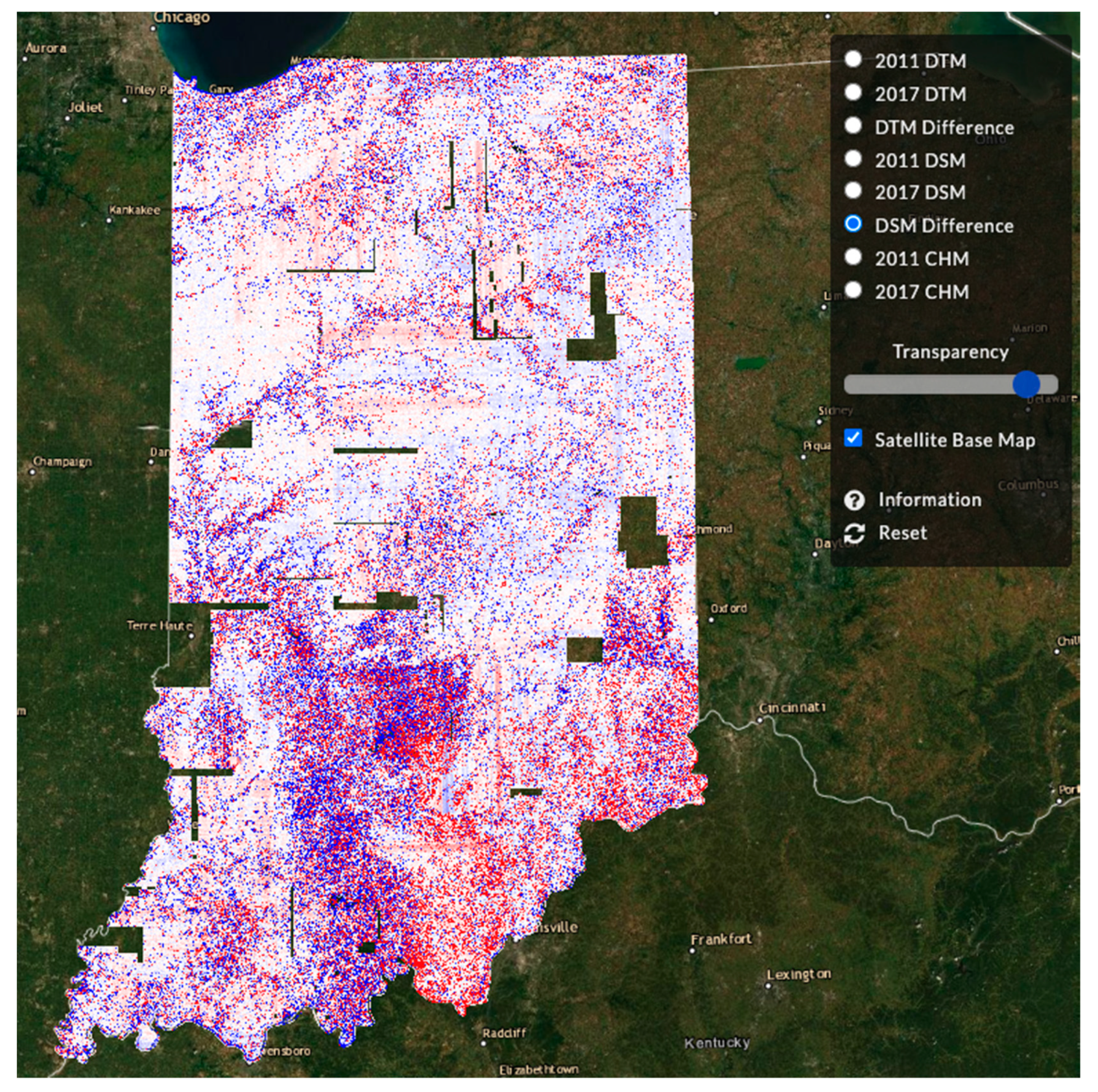
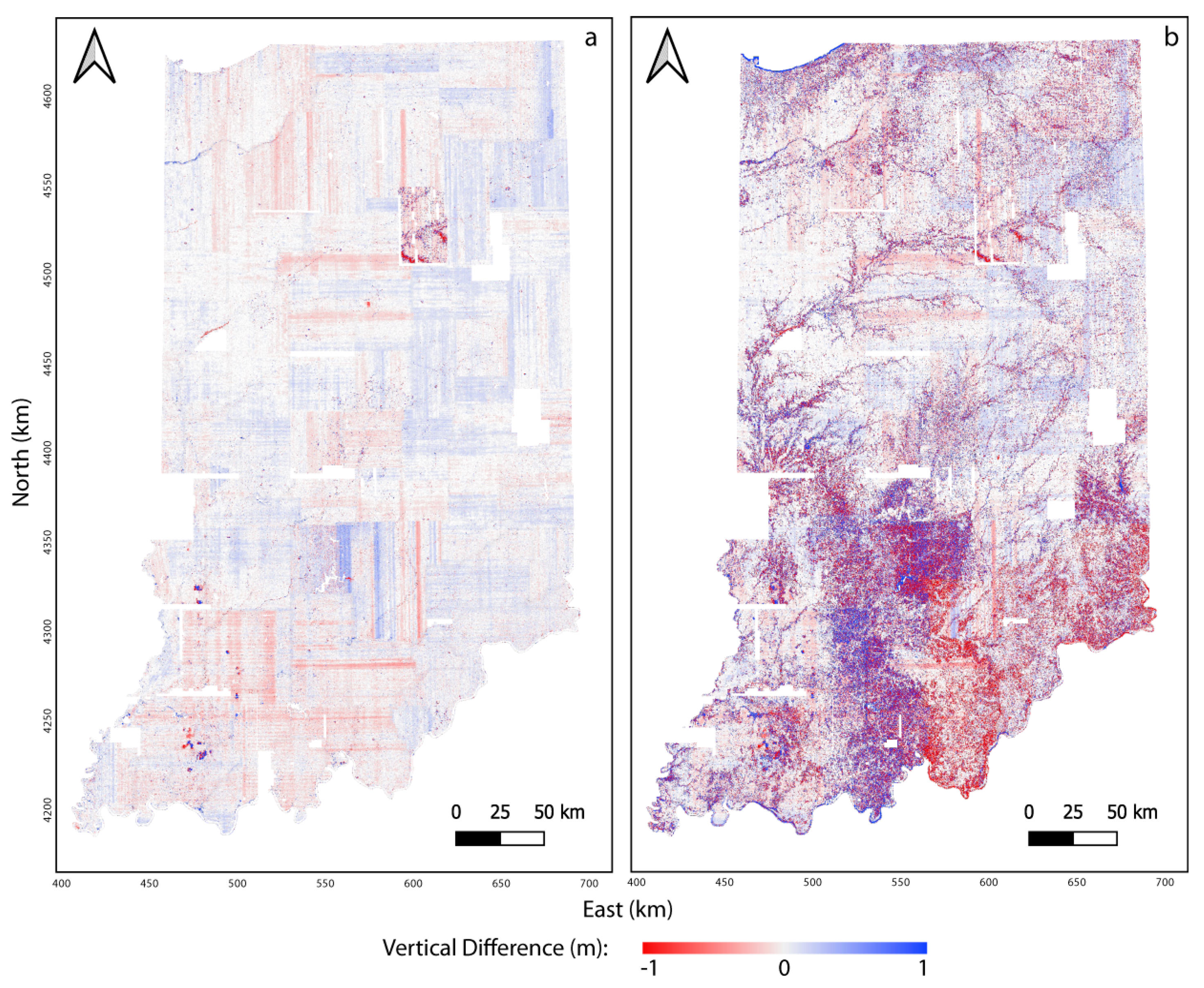
2.3. Vertical Raster-Based Differencing

Vertical raster-based differencing can be performed on raster DTMs and DSMs with identical origins, boundaries, and resolution. The earlier dataset is the ‘compare,’ and the later dataset is the ‘reference’ [19]. The vertical difference is a raster subtraction:

$$Z_{Difference=Z_{reference}-Z_{compare},}$$

(2)

where $Z_{reference}$ and $Z_{compare}$ are the DSMs or DTMs acquired at different dates, and $Z_{Difference}$ is the differenced raster. Because topographic change can be on the same order of magnitude as dataset errors, errors in the surveying, point classification, and metadata (i.e., coordinate reference system (CRS) and epoch) often become pronounced.

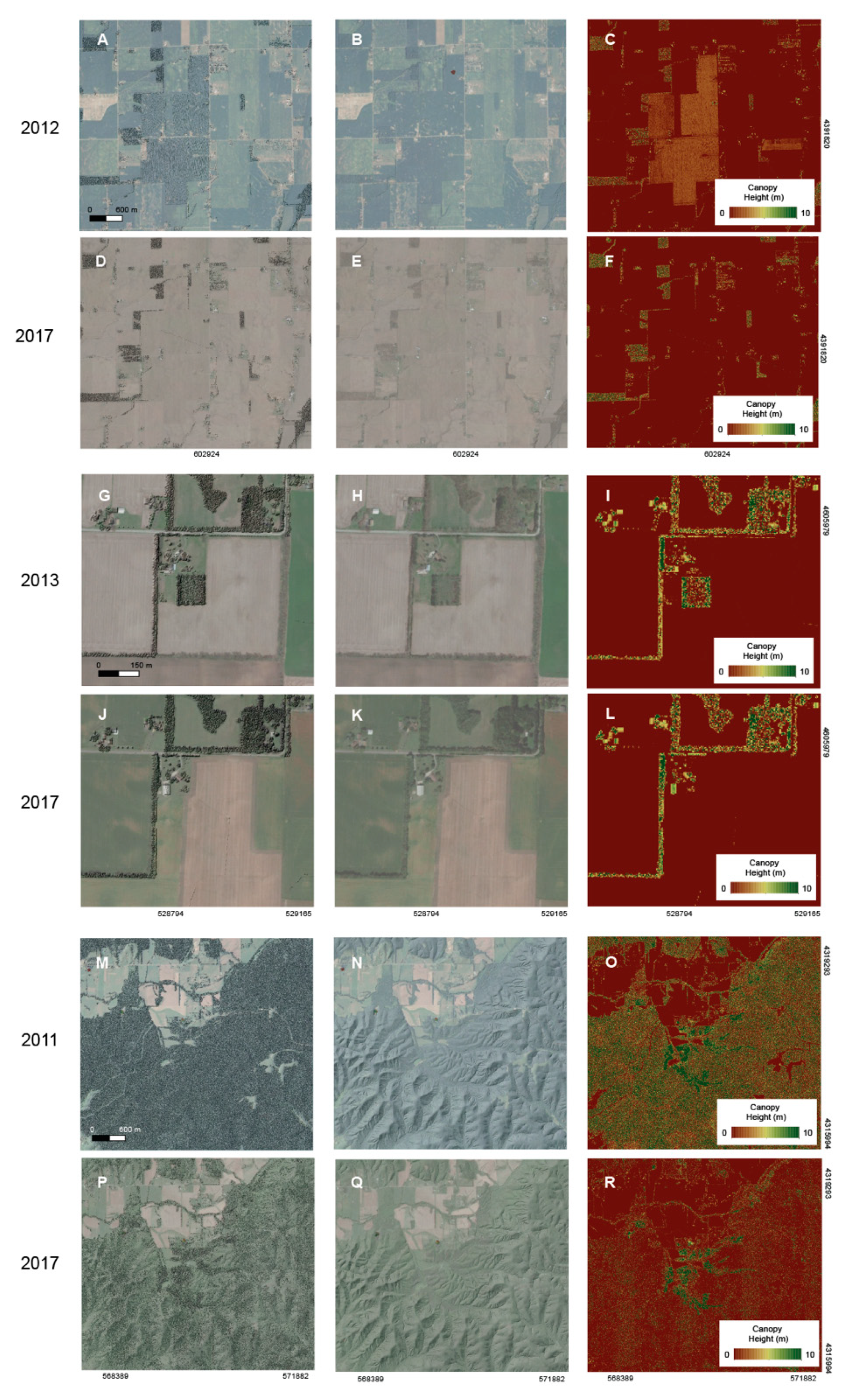
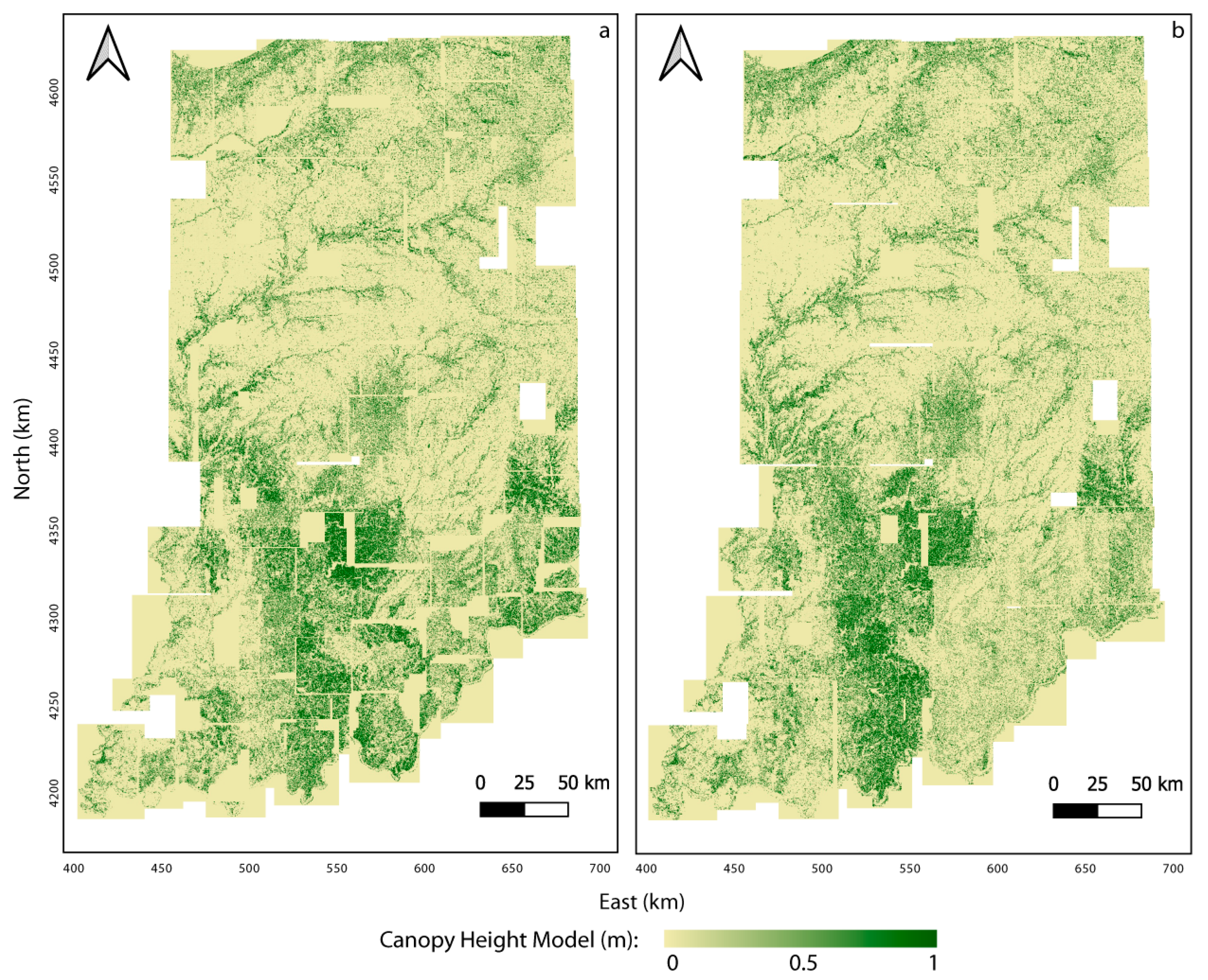
2.4. Canopy Height Model

A canopy height model (CHM) or normalized DSM (nDSM) measures the height of vegetation and buildings above the ground. A common and straightforward approach to calculate a CHM is to subtract the DTM from the DSM acquired at the same time:

CHM = DSM – DTM

(3)

We use this approach, which follows naturally from the vertical differencing. However, this approach has errors when the DTM and DSM do not represent the ground surface [47] and the top of the landscape, respectively. There are other approaches to calculate the CHM—for example, the interpolation of the full point cloud dataset to calculate the position of the ground beneath non-ground points [48].

3. Datasets

The 2011–2013 Indiana lidar dataset [20] was collected by IndianaMap and became part of the U.S. Geological Survey’s Lidar Point Cloud project, which preceded their 3DEP project. It was collected county by county from 2011 to 2013 and covers a total of 94,000 km² with an average point density of 1.6 pts/m². The dataset includes 149 × 10⁹ lidar returns, and 44% of these points are classified as ground (i.e., LAS class 2). The dataset was originally delivered in State Plane CRS with units of U.S. feet and with different EPSG codes for the eastern and western portions of the state. We accessed the data in Entwine Point Tiles (EPT) format (https://entwine.io (accessed on 1 July 2021)) via the Amazon Web Services (AWS) Simple Storage Service (S3) Public Dataset bucket (https://registry.opendata.aws/usgs-lidar/ (accessed on 1 July 2021)). The dataset was published by the USGS with a horizontal CRS of WGS84 Web Mercator (EPSG: 3857) and a vertical CRS of the North American Vertical Datum (NAVD) 88 with the GEOID09 datum. The dataset is also available through OpenTopography as well as The National Map, where it is saved on the county scale, as shown in Figure 3A.

The USGS 3DEP Indiana lidar dataset was collected between 2016 and 2020 and is also available through the AWS Public Dataset S3 bucket in EPT format. The dataset is USGS Quality Level 2, implying a 10 cm vertical accuracy and at least 2 pts/m². The horizontal CRS is the same as the 2011–2013 dataset, WGS84 (EPSG: 3857). The vertical CRS is the North American Vertical Datum (NAVD) 88 with the GEOID12 datum and units of meters. The 2016–2020 lidar collection is saved in multiple files, each of which typically spans multiple counties, although the dataset boundaries do not strictly follow county lines, as shown in Figure 3B.

4. Methods

We developed a largely automated workflow to generate DTM and DSM change and CHM maps of Indiana from the classified lidar point cloud datasets. In this section, we outline the main steps of the workflow, as shown in Figure 4. The resulting statewide differencing maps are shown in Figure 1, statewide CHM maps are shown in Figure 2, and Figure 5, Figure 6 and Figure 7 show example areas of notable DTM, DSM, and CHM change, respectively.

We accessed both Indiana lidar point cloud topography datasets from an AWS public dataset S3 bucket using a Point Data Abstraction Library (PDAL) processing pipeline [49]. At the download step, we reprojected the data in the native Web Mercator (EPSG 3857) horizontal CRS to Universal Transverse Mercator (UTM) Zone 16 (WGS84 Ellipsoid), EPSG 32616. Web Mercator (EPSG 3857) is a standard projection for web mapping applications, but is not ideal for most mapping applications because of the high area distortions. The UTM CRS has very little distortion (>1/1000 m/m) within individual zones. We found that downloading the data in 4 km² tiles from the AWS bucket was optimal and avoided rare time-out issues with any larger areas, which would in turn require a complete restart of that process.

For efficient memory management, we divided each county into four parts and downloaded the 4 km² tiles of data that spanned each of the quarters. We used LAStool’s ‘lastile’ [50] to retile the quarter county data into 1 km² tiles. Although LAStool’s ‘lastile’ could handle large datasets well, the command sometimes failed without an error or warning message when applied to full counties.

We generated 1 km² DSMs and DTMs for both acquisitions. Both lidar datasets were classified by the dataset vendor prior to delivery with common point classifications, including unclassified (LAS class 1), ground (class 2), low to high vegetation (classes 3–5), building (class 6), noise (class 7), water (class 9), rail (class 10), road surface (class 11), overlap (class 12), wire (class 13), and transmission tower (class 15). We did not pursue point cloud reclassification because both datasets underwent a quality control review by the State of Indiana and USGS prior to delivery. To extract the ground points, we used LAStools’ ‘las2las’ [50] with the option to keep ground points. We generated one-meter-resolution raster DSMs and DTMs with LAStool’s ‘las2dem’, which uses a triangular irregular network (TIN) approach [51]. We preferred the 1 km² tile area generated with lastile because the gridding step was performed efficiently, and 1 km-square tiles worked well in the visualization steps. We ensured that the datasets had the same bounds even along county boundaries with GDAL’s ‘gdalwarp’ [52].

The geoid epochs of the two datasets differ: the 2011–2013 dataset is in GEOID09 while the 2016–2020 dataset is in GEOID12B. Using GDAL’s ‘gdalwarp’, we performed a vertical CRS transformation to remove the appropriate GEOID from the raster-based heights, resulting in ellipsoidal height elevations.

We generated topographic differencing (Equation (2)) CHM (Equation (3)) maps with GDAL’s ‘gdal_calc’. Areas of no data occur above water in DTMs and immediately outside of county boundaries and have values of −9999.

There are inconsistent dataset names and several partially empty datasets in the AWS S3 public bucket. Manually correcting these dataset names makes the algorithm less automated. We performed no differencing over the western portion of the counties Vigo, Wayne, and Wells where data are missing.

Easy access and visualization of large statewide differencing datasets poses its own set of challenges. Our objective was to make the data browsable and explorable through an easy-to-use web interface that can be viewed concurrently by users with varying geospatial ability and experience. We utilized the open-source application server Geoserver (geoserver.org) to publish a Web Mapping Service (WMS) of the statewide differencing data products, as shown in Figure 8. To leverage Geoserver and its visualization capabilities, we prepared each raster dataset (i.e., two DTMs, two DSMs, DTM change, DSM change, and two CHMs) by applying compression, developing a tiling scheme, and adding overviews. File tiling reduces access time by eliminating the need to read through an entire file before subsetting the necessary pixels. With tiling, access requests can simply find the appropriate tile(s) and efficiently subset an area of interest from those tiles. Overviews allow the user to quickly pan and zoom within the map by setting up a ‘pyramid’ of tiled mosaics. The overviews improve performance, which is critical for the end user experience when visualizing large data volumes. Our WMS of the Indiana differencing products is available here: https://doi.org/10.5069/G9MG7MQV (accessed on 1 July 2021).

5. Results

In this section, we discuss the differencing and CHM results at the statewide and site scales. The visually most dominant signal in the statewide DTM change map (Figure 1a) is the north–south- and east–west-oriented blue and red stripes. These stripes do not represent real topographic change but instead indicate misalignment between data collected along adjacent flight paths. These errors are likely from the 2011–2013 dataset because the errors correlate with the county boundaries that guided the earlier acquisition (Figure 3A). While these errors can be corrected [22,42], the correction benefits from flight trajectory data are very time-intensive and are out of scope for most large-scale studies. Topographically correlated errors vary with slope direction—for example, in Brown County in South–Central Indiana. This apparent lateral shift reflects horizontal georeferencing errors.

Physical changes visible on both statewide differencing maps include mining and quarrying concentrated change near the western and southern state borders. The Wabash and White rivers create south–west-oriented patterns that stretch across the central and southern portions of the state and are produced by fluvial, riparian, and anthropogenic activity. In the south–central portion of the state DSM change map, the color variation along a north–south boundary reflects the seasons of the lidar acquisitions. Purple (west) indicates data acquisition during similar seasons, and red (east) indicates leaf-on to leaf-off conditions.

The statewide CHM maps (Figure 2) indicate landscape type, including agriculture in the center and north, forests such as the Hoosier National Forest in South–Central Indiana and in the northwest by Lake Michigan, and the riparian zones along major rivers. The variability between the two CHM maps in Southeast Indiana reflects a foliage change associated with the seasons of dataset acquisition.

In the remainder of the section, we discuss site-scale examples of DTM change, DSM change, and the CHM. For the DTM change, rivers and riparian zones are very dynamic (Figure 5A–C), as illustrated for the Wabash River in the southwestern-most part of Indiana. Oxbow lakes are developing, and the change map shows a signal that is likely a combination of sediment deposition, erosion along the meander core, as well as flight alignment errors. A shale and limestone quarry located north of Louisville, Indiana, also produces height changes up to a few tens of meters (Figure 5D–F). The change map shows the movement and removal of stone in the active quarry, and, as expected, the overwhelming red color indicates that material is net-removed. The Indiana Dunes National Park and other areas along Lake Michigan’s shoreline (Figure 5G–I) have been impacted by nearby industry, including coal-fired power plants, logging, farming, and suppressed burns, and thus have a high propensity for erosion, especially during recent high-water levels in the lake [53]. The National Parks Service is working to restore portions of the wetland areas, and the differenced DTM shows that the largest changes occurred along the beach where there is no vegetation. Sinkholes near Mitchell, Indiana, also produce significant change [54], as shown in Figure 5J–L. These sinkholes are represented by the circular features in the hillshades. The red and blue circles in the differencing plot show that sinkholes, sometimes ~20 m deep, have formed or have been filled in between the lidar acquisitions.

Here, we discuss DSM change. Figure 6A–C shows a new housing development in an Indianapolis suburb, where the maximum height of the new houses is ~10 m. Change is created by highway construction, where an overpass was replaced with a partial clover intersection and ramps bend approaching the intersection (Figure 6D–F). Figure 6G–I show a crane adjacent to ongoing construction at the Memorial Stadium at Indiana University. The Indiana Harbor and Ship Canal is home to one of the largest steel-making facilities in North America (Figure 6K,L), and the change reflects the movement of material. Agriculture causes landscape change (Figure 6M–O), and the blue squares are new farm buildings. A decrease in elevation along vegetation implies vegetation loss.

The CHM derived from the 2012 lidar acquisition over Fountaintown, Indiana, shows a field of ~2.5 m tall crops and surrounding ~5–8 m tall trees (Figure 7C), reflecting the summer acquisition. The CHM from the March–April 2017 lidar shows the same trees but does not show any crops due to acquisition before the summer (Figure 7F). Comparisons of CHM acquired during different years also show changes in land use and timber harvesting: the CHM from 2013 over La Porte, Indiana, shows trees that are absent in the 2017 CHM, indicating that the trees had been removed between the acquisitions (Figure 7I,L). The 2011 CHM acquired near Houston, Indiana, shows dense forest cover and trees up to ~10 m tall (Figure 7O). The 2017 CHM shows a reduction in vegetation density and tree coverage (Figure 7R). These observations reflect leaf-on (2011) and leaf-off conditions (2017).

6. Discussion

6.1. Large-Scale Topographic Differencing Challenges

We demonstrated the successful statewide topographic differencing of meter-scale resolution lidar topography. As with most Big Data Earth observation projects, we faced multiple challenges in accessing, processing, and analyzing the data. These include:

(1) The statewide DTMs, DSMs, DTM and DSM differencing, and CHM products together generated ~4 terabytes of final raster products. The intermediate products were of a similar scale because we saved the point clouds as compressed laz and not as larger las products. This required ~10 TB of local disk space that had to be readily available throughout the project.

(2) The intermediate point cloud products required careful management to ensure efficient allocation of the fixed memory available for the processing. Even popular software packages such as LAStools can have difficulty working with larger county-scale datasets. This fact emphasizes the Big Data challenges that are common to the processing and analysis of large-scale and high-resolution datasets.

(3) Once the processing workflow was established and associated technical challenges overcome, we estimated that the statewide differencing workflow would have taken approximately one year of compute time if it were running on a commodity server or local workstation. This aspect emphasizes the need for dedicated high-performance computing resources with large memory and multicore CPUs for faster processing and more reasonable timelines for analysis. Although relatively infrequent, the processing did stop, sometimes requiring a manual restart, which benefited from a modular workflow design that enabled relatively efficient failure recovery.

(4) The nature of the project management for the lidar acquisitions meant that the data were acquired over a range of dates, in irregular spatial patterns, and with inconsistent data characteristics. A dedicated data acquisition effort for state scale differencing could be designed to provide consistent data quality and organization that would more efficiently yield the differencing products discussed here.

(5) The largest source of noise is the offset between flight-lines in the lidar data, which appear as east–west- and north–south-oriented swaths most noticeable in the differenced DTM (Figure 1a). This type of error can be corrected using additional flight trajectory information [42]. However, this process is at best very time-intensive and requires flight information that is rarely delivered with the topography data, and thus would likely be challenging to locate at the state scale. Georeferencing errors also produce topographically correlated noise. We made the explicit choice to not correct these errors because the correction is out of scope for this project and the majority of the change signals are larger than the noise amplitude. This choice was also an opportunity to explore the overall quality of these statewide datasets and to better understand their suitability for multi-temporal analyses without additional and labor-intensive adjustments. In the case of Indiana, these flight-line errors appear to be largely present in the earlier lidar dataset. This observation is consistent with the general observation that older and legacy lidar datasets have larger errors and lower resolution. Thanks to improvements in lidar technology, as well as the data quality control and review processes, these types of errors are likely to be less prevalent in future dataset collections. We expect that this topographic differencing exercise presents a common set of challenges that would face any large-scale analysis of 3DEP or similar regional to national scale topography datasets.

These noise sources impose a limitation to the utility of the Indiana statewide datasets. We expect that our results are useful for detecting change and conducting scientific analyses at regional or statewide scales of signals whose amplitude exceeds that of the noise with spatially heterogeneous characteristics. Studies on the site scale or of lower-amplitude signals are likely to benefit from focused approaches to mitigate noise, such as the correction of the flight alignment, georeferencing, or point classification errors [22,42,44,50].

(6) Visualizing Big Data results is challenging, especially for those without an extensive geospatial background. Our Web Mapping Service visualization (Figure 8) demonstrates an approach to sharing Big Data studies, which is important for results such as these to be well communicated and possibly used to inform policy [2]. We expect that the web-based, easy-to-access visualization of our results will lead to a broader utilization of our work, especially in education [55] and by state and local policy makers.

6.2. Future Topographic Differencing

Thanks to the USGS 3DEP and other large-scale lidar mapping initiatives, there are now significant portions of the United States and the world covered by repeat, high-resolution, airborne and spaceborne topography datasets collected over the past decade. As shown in Figure 9, our analysis of USGS 3DEP and the U.S. Interagency Elevation Inventory (ISIEI) datasets shows that at least ~37% of the lower 48 of the United States is covered by open, repeat lidar. Topographic differencing is likely possible in additional areas by differencing 3DEP with other open data datasets, by incorporating datasets that are nominally public yet difficult to access, or by performing hybrid differencing with satellite topography datasets [21] that typically have a larger footprint than most lidar acquisitions.

While this growing body of open data presents a great opportunity for performing topographic differencing analyses, the large-scale integration of types and vintages of datasets brings new challenges. First, the repeat topographic data will likely have different characteristics, including resolution, noise, and sensitivity to vegetation. These differences are especially likely to be exacerbated for hybrid datasets. An approach for differencing modern and legacy lidar includes setting the resolution of the differencing product based on the lower-resolution dataset [28], as we do here. Second, the lack of a single, centralized repository for topographic data makes finding, accessing, and processing topography datasets originally acquired by a range of organizations challenging. Initiatives such as the 3DEP, the USIEI, and OpenTopography are improving this situation, but significant funding and political challenges exist in centralizing access to high resolution topography, particularly for legacy datasets collected and housed by numerous governmental entities. Third, performing differencing on increasingly large scales is a classic Big Data challenge with the requisite requirements for compute and storage. High-performance computing (HPC) and cloud infrastructure provide a pathway, but fundamental updates are necessary to data archive, access, and processing systems to fully enable big topographic data analysis. In addition, technical issues such as quality and detailed metadata, coordinate reference systems, consistency of point cloud classifications, and improvement of legacy dataset alignment can present serious obstacles if not dealt with correctly.

6.3. Other Large-Scale Processing

Big Data analyses of remote sensing datasets are becoming increasingly common and necessary to efficiently analyze large-scale geospatial data. For example, Constantini et al. [11] developed a time-series of surface deformation rates from Interferometric Synthetic Aperture Radar (InSAR) over all of Italy and discussed the importance of national databases of terrain movement and the associated challenges related to workflow development, efficient use of HPC resources, noise correction, and ground truthing. Bhangale et al. [10] implemented HPC resources to detect oil spills from multi-temporal Landsat datasets and characterized the computational gains from graphics processing units (GPUs).

Insights into Big Data processing from studies such as those discussed above and our work can provide support for a variety of activities in Earth observation. For example, these and similar methods could be applied to the mapping of geologic hazards including landslides [56], sinkholes [57], flood zones [7], tectonic faults [58,59], and coastal erosion [9]. They can also be applied to understand anthropogenic interaction with the environment—for example, biomass or biomass change [6,47,60,61], agriculture [62], and infrastructure development [8]. Increasing the complexity from the quantification of change to semantic variation over time (types and drivers of vertical variation in topography or canopy height structure) can come from additional analysis using machine learning tools [63].

7. Conclusions

In this paper, we presented the first statewide topographic differencing analysis using publicly available lidar high-resolution topography from the State of Indiana (2011–2013 dataset) and U.S. Geological Survey’s 3DEP (2016–2020 dataset). We discussed a range of Big Data challenges that we overcame, including accessing the datasets, developing an automated differencing workflow, allocating sufficient compute resources, and managing the data products and their visualization. The statewide differencing results show flight-line alignment errors that are likely from the earlier lidar acquisition and highlight the challenges that these errors pose in large-scale analyses. We documented landscape changes from fluvial activity, vegetation changes, and infrastructure development. As the 3DEP topography collection grows and increasingly more areas are covered with single and repeat topography, large-scale analyses such as ours will be critical to characterizing the Earth’s landscape and its changes over time.

References

1. Casu, F.; Manunta, M.; Agram, P.S.; Crippen, R.E. Big Remotely Sensed Data: Tools, Applications and Experiences. Remote Sens. Environ. 2017, 202, 1–2. [Google Scholar] [CrossRef]
2. Runting, R.K.; Phinn, S.; Xie, Z.; Venter, O.; Watson, J.E.M. Opportunities for Big Data in Conservation and Sustainability. Nat. Commun 2020, 11, 2003. [Google Scholar] [CrossRef]
3. Loveland, T.R.; Dwyer, J.L. Landsat: Building a Strong Future. Remote Sens. Environ. 2012, 122, 22–29. [Google Scholar] [CrossRef]
4. Showstack, R. Sentinel Satellites Initiate New Era in Earth Observation. Eos Trans. AGU 2014, 95, 239–240. [Google Scholar] [CrossRef]
5. U.S. Geological Survey Lidar Point Cloud—USGS National Map 3DEP Downloadable Data Collection. U.S. Geol. Surv. 2018. Available online: https://www.usgs.gov/programs/national-geospatial-program/national-map (accessed on 1 July 2021).
6. Chuvieco, E.; Mouillot, F.; van der Werf, G.R.; San Miguel, J.; Tanase, M.; Koutsias, N.; García, M.; Yebra, M.; Padilla, M.; Gitas, I.; et al. Historical Background and Current Developments for Mapping Burned Area from Satellite Earth Observation. Remote Sens. Environ. 2019, 225, 45–64. [Google Scholar] [CrossRef]
7. Guerriero, L.; Ruzza, G.; Guadagno, F.M.; Revellino, P. Flood Hazard Mapping Incorporating Multiple Probability Models. J. Hydrol. 2020, 587, 125020. [Google Scholar] [CrossRef]
8. Kruitwagen, L.; Story, K.T.; Friedrich, J.; Byers, L.; Skillman, S.; Hepburn, C. A Global Inventory of Photovoltaic Solar Energy Generating Units. Nature 2021, 598, 604–610. [Google Scholar] [CrossRef]
9. Murray, N.J.; Phinn, S.R.; DeWitt, M.; Ferrari, R.; Johnston, R.; Lyons, M.B.; Clinton, N.; Thau, D.; Fuller, R.A. The Global Distribution and Trajectory of Tidal Flats. Nature 2019, 565, 222–225. [Google Scholar] [CrossRef]
10. Bhangale, U.; Durbha, S.S.; King, R.L.; Younan, N.H.; Vatsavai, R. High Performance GPU Computing Based Approaches for Oil Spill Detection from Multi-Temporal Remote Sensing Data. Remote Sens. Environ. 2017, 202, 28–44. [Google Scholar] [CrossRef]
11. Costantini, M.; Ferretti, A.; Minati, F.; Falco, S.; Trillo, F.; Colombo, D.; Novali, F.; Malvarosa, F.; Mammone, C.; Vecchioli, F.; et al. Analysis of Surface Deformations over the Whole Italian Territory by Interferometric Processing of ERS, Envisat and COSMO-SkyMed Radar Data. Remote Sens. Environ. 2017, 202, 250–275. [Google Scholar] [CrossRef]
12. Albino, F.; Smets, B.; d’Oreye, N.; Kervyn, F. High-Resolution TanDEM-X DEM: An Accurate Method to Estimate Lava Flow Volumes at Nyamulagira Volcano (D. R. Congo): TANDEM-X DEM TO DERIVE LAVA FLOW VOLUMES. J. Geophys. Res. Solid Earth 2015, 120, 4189–4207. [Google Scholar] [CrossRef] [Green Version]
13. Bull, J.M.; Miller, H.; Gravley, D.M.; Costello, D.; Hikuroa, D.C.H.; Dix, J.K. Assessing Debris Flows Using LIDAR Differencing: 18 May 2005 Matata Event, New Zealand. Geomorphology 2010, 124, 75–84. [Google Scholar] [CrossRef] [Green Version]
14. Dietterich, H.R.; Diefenbach, A.K.; Soule, S.A.; Zoeller, M.H.; Patrick, M.P.; Major, J.J.; Lundgren, P.R. Lava Effusion Rate Evolution and Erupted Volume during the 2018 Kīlauea Lower East Rift Zone Eruption. Bull. Volcanol. 2021, 83, 25. [Google Scholar] [CrossRef]
15. Izumida, A.; Uchiyama, S.; Sugai, T. Application of UAV-SfM Photogrammetry and Aerial Lidar to a Disastrous Flood: Repeated Topographic Measurement of a Newly Formed Crevasse Splay of the Kinu River, Central Japan. Nat. Hazards Earth Syst. Sci. 2017, 17, 1505–1519. [Google Scholar] [CrossRef] [Green Version]
16. Scott, C.P.; Arrowsmith, J.R.; Nissen, E.; Lajoie, L.; Maruyama, T.; Chiba, T. The M 7 2016 Kumamoto, Japan, Earthquake: 3-D Deformation along the Fault and Within the Damage Zone Constrained From Differential Lidar Topography. J. Geophys. Res. Solid Earth 2018, 123, 6138–6155. [Google Scholar] [CrossRef]
17. Scott, C.P.; DeLong, S.B.; Arrowsmith, J.R. Distribution of Aseismic Deformation Along the Central San Andreas and Calaveras Faults from Differencing Repeat Airborne Lidar. Geophys. Res. Lett. 2020, 47, 1–10. [Google Scholar] [CrossRef]
18. Wedmore, L.N.J.; Gregory, L.C.; McCaffrey, K.J.W.; Goodall, H.; Walters, R.J. Partitioned Off-Fault Deformation in the 2016 Norcia Earthquake Captured by Differential Terrestrial Laser Scanning. Geophys. Res. Lett. 2019, 46, 3199–3205. [Google Scholar] [CrossRef] [Green Version]
19. Wheaton, J.M.; Brasington, J.; Darby, S.E.; Sear, D.A. Accounting for Uncertainty in DEMs from Repeat Topographic Surveys: Improved Sediment Budgets. Earth Surf. Processes Landf. 2009, 35, 136–156. [Google Scholar] [CrossRef]
20. Indiana Map 2011–2013 Indiana Statewide LiDAR. Open Topography 2012. [CrossRef]
21. Barnhart, W.D.; Gold, R.D.; Shea, H.N.; Peterson, K.E.; Briggs, R.W.; Harbor, D.J. Vertical Coseismic Offsets Derived from High-Resolution Stereogrammetric DSM Differencing: The 2013 Baluchistan, Pakistan Earthquake. J. Geophys. Res. Solid Earth 2019, 124, 6039–6055. [Google Scholar] [CrossRef]
22. DeLong, S.; Engle, Z.; Hammer, M.; Scott, C.P.; Arrowsmith, J.R. Regional-Scale Landscape Change: Data Preparation and Two Examples Using Object-Based Image Analysis and Windowed Iterative Closest Point Algorithm to Interrogate Results. In Proceedings of the AGU Fall Meeting Abstracts, Washington, DC, USA, 7 December 2020. [Google Scholar]
23. Hilgendorf, Z.; Marvin, M.C.; Turner, C.M.; Walker, I.J. Assessing Geomorphic Change in Restored Coastal Dune Ecosystems Using a Multi-Platform Aerial Approach. Remote Sens. 2021, 13, 354. [Google Scholar] [CrossRef]
24. Scott, C.; Bunds, M.; Shirzaei, M.; Toke, N. Creep along the Central San Andreas Fault from Surface Fractures, Topographic Differencing, and InSAR. J. Geophys. Res. Solid Earth 2020, 125, 1–16. [Google Scholar] [CrossRef]
25. Crosby, C.J.; Arrowsmith, J.R.; Nandigam, V. Chapter 11—Zero to a Trillion: Advancing Earth Surface Process Studies with Open Access to High-Resolution Topography. In Remote Sensing of Geomorphology; Developments in Earth Surface Processes; Elsevier: Amsterdam, The Netherlands, 2020; Volume 33, pp. 317–338. [Google Scholar]
26. Crosby, C.J.; Arrowsmith, J.R.; Nandigam, V.; Baru, C. Online Access and Processing of LiDAR Topography Data. In Geoinformatics; Keller, G.R., Baru, C., Eds.; Cambridge University Press: Cambridge, UK, 2011; pp. 251–265. ISBN 978-0-511-97630-8. [Google Scholar]
27. Krishnan, S.; Crosby, C.; Nandigam, V.; Phan, M.; Cowart, C.; Baru, C.; Arrowsmith, R. OpenTopography: A Services Oriented Architecture for Community Access to LIDAR Topography. In Proceedings of the 2nd International Conference on Computing for Geospatial Research & Applications—COM.Geo ’11, Washington, DC, USA, 23–25 May 2011; ACM Press: Washington, DC, USA, 2011; pp. 1–8. [Google Scholar]
28. Scott, C.; Phan, M.; Nandigam, V.; Crosby, C.; Arrowsmith, J.R. Measuring Change at Earth’s Surface: On-Demand Vertical and Three-Dimensional Topographic Differencing Implemented in Open Topography. Geosphere 2021, 17, 1318–1332. [Google Scholar] [CrossRef]
29. Oskin, M.E.; Arrowsmith, J.R.; Corona, A.H.; Elliott, A.J.; Fletcher, J.M.; Fielding, E.J.; Gold, P.O.; Garcia, J.J.G.; Hudnut, K.W.; Liu-Zeng, J.; et al. Near-Field Deformation from the El Mayor-Cucapah Earthquake Revealed by Differential LIDAR. Science 2012, 335, 702–705. [Google Scholar] [CrossRef] [Green Version]
30. Bellekens, B.; Spruyt, V.; Berkvens, R.; Maarten, W. A Survey of Rigid 3D Pointcloud Registration Algorithms. In Proceedings of the AMBIENT 2014: The Fourth International Conference on Ambient Computing, Applications, Services and Technologies, Rome, Italy, 24–28 August 2014. [Google Scholar]
31. Besl, P.J.; McKay, N.D. A Method for Registration of 3-D Shapes. IEEE Trans. Pattern Anal. Mach. Intell. 1992, 14, 239–256. [Google Scholar] [CrossRef]
32. Nissen, E.; Maruyama, T.; Ramon Arrowsmith, J.; Elliott, J.R.; Krishnan, A.K.; Oskin, M.E.; Saripalli, S. Coseismic Fault Zone Deformation Revealed with Differential Lidar: Examples from Japanese ∼7 Intraplate Earthquakes. Earth Planet. Sci. Lett. 2014, 405, 244–256. [Google Scholar] [CrossRef]
33. Lague, D.; Brodu, N.; Leroux, J. Accurate 3D Comparison of Complex Topography with Terrestrial Laser Scanner: Application to the Rangitikei Canyon (N-Z). ISPRS J. Photogramm. Remote Sens. 2013, 82, 10–26. [Google Scholar] [CrossRef] [Green Version]
34. Farr, T.G.; Rosen, P.A.; Caro, E.; Crippen, R.; Duren, R.; Hensley, S.; Kobrick, M.; Paller, M.; Rodriguez, E.; Roth, L.; et al. The Shuttle Radar Topography Mission. Rev. Geophys. 2007, 45, 1–33. [Google Scholar] [CrossRef] [Green Version]
35. Ekhtari, N.; Glennie, C. High-Resolution Mapping of Near-Field Deformation with Airborne Earth Observation Data, a Comparison Study. IEEE Trans. Geosci. Remote Sens. 2017, 56, 1–17. [Google Scholar] [CrossRef]
36. Glennie, C. Rigorous 3D Error Analysis of Kinematic Scanning LIDAR Systems. J. Appl. Geod. 2007, 1, 147–157. [Google Scholar] [CrossRef]
37. Goulden, T.; Hopkinson, C. The Forward Propagation of Integrated System Component Errors within Airborne Lidar Data. Photogramm. Eng. Remote Sens. 2010, 76, 589–601. [Google Scholar] [CrossRef]
38. Toth, C.; Brzezinska, D.; Csanyi, N.; Paska, E.; Yastikli, N. LiDAR Mapping Sup-Porting Earthquake Research of the San Andreas Fault. In Proceedings of the ASPRS 2007 Annual Conference. American Society for Photogrammetry and Remote Sensing, Tampa, FL, USA, 7–11 May 2007; pp. 1–11. [Google Scholar]
39. Liu, X. Airborne LiDAR for DEM Generation: Some Critical Issues. Prog. Phys. Geogr. Earth Environ. 2008, 32, 31–49. [Google Scholar] [CrossRef]
40. Hodgson, M.E.; Bresnahan, P. Accuracy of Airborne Lidar-Derived Elevation. Photogramm. Eng. Remote Sens. 2004, 70, 331–339. [Google Scholar] [CrossRef] [Green Version]
41. Shan, S.; Bevis, M.; Kendrick, E.; Mader, G.L.; Raleigh, D.; Hudnut, K.; Sartori, M.; Phillips, D. Kinematic GPS Solutions for Aircraft Trajectories: Identifying and Minimizing Systematic Height Errors Associated with Atmospheric Propagation Delays. Geophys. Res. Lett. 2007, 34. [Google Scholar] [CrossRef] [Green Version]
42. Glennie, C.L.; Hinojosa-Corona, A.; Nissen, E.; Kusari, A.; Oskin, M.E.; Arrowsmith, J.R.; Borsa, A. Optimization of Legacy Lidar Data Sets for Measuring Near-Field Earthquake Displacements. Geophys. Res. Lett. 2014, 41, 3494–3501. [Google Scholar] [CrossRef]
43. El-Sheimy, N.; Valeo, C.; Habib, A. Digital Terrain Modeling: Acquisition, Manipulation, and Applications; Artech House: Boston, MA, USA, 2005; p. 270. [Google Scholar]
44. Passalacqua, P.; Belmont, P.; Staley, D.M.; Simley, J.D.; Arrowsmith, J.R.; Bode, C.A.; Crosby, C.; DeLong, S.B.; Glenn, N.F.; Kelly, S.A.; et al. Analyzing High Resolution Topography for Advancing the Understanding of Mass and Energy Transfer through Landscapes: A Review. Earth-Sci. Rev. 2015, 148, 174–193. [Google Scholar] [CrossRef] [Green Version]
45. Brasington, J.; Langham, J.; Rumsby, B. Methodological Sensitivity of Morphometric Estimates of Coarse Fluvial Sediment Transport. Geomorphology 2003, 53, 299–316. [Google Scholar] [CrossRef]
46. Smith, T.; Rheinwalt, A.; Bookhagen, B. Determining the Optimal Grid Resolution for Topographic Analysis on an Airborne Lidar Dataset. Earth Surf. Dyn. 2019, 7, 475–489. [Google Scholar] [CrossRef] [Green Version]
47. Roussel, J.-R.; Auty, D.; Coops, N.C.; Tompalski, P.; Goodbody, T.R.H.; Meador, A.S.; Bourdon, J.-F.; de Boissieu, F.; Achim, A. LidR: An R Package for Analysis of Airborne Laser Scanning (ALS) Data. Remote Sens. Environ. 2020, 251, 112061. [Google Scholar] [CrossRef]
48. García, V.H.; Hongn, F.; Cristallini, E.O. Late Miocene to Recent Morphotectonic Evolution and Potential Seismic Hazard of the Northern Lerma Valley: Clues from Lomas de Medeiros, Cordillera Oriental, NW Argentina. Tectonophys 2013, 608, 1238–1253. [Google Scholar] [CrossRef]
49. PDAL Contributors PDAL Point Data Abstraction Library; Zenodo. 2018. Available online: https://zenodo.org/record/2556738#.YgXM6v5ByUk (accessed on 1 July 2021).
50. Isenburg, M. LAStools—Efficient Tools for Lidar Processing. 2019. Available online: https://rapidlasso.com/lastool (accessed on 1 July 2021).
51. Isenburg, M.; Liu, Y.; Snoeyink, J.; Thirion, T. Generating Raster DEM from Mass Points via TIN Streaming. In Proceedings of the GIScience’06 Conference Proceedings, Münster, Germany, 20–23 September 2006; Springer: Berlin/Heidelberg, Germany, 2006; pp. 186–198. [Google Scholar]
52. GDAL/OGR Contributors GDAL/OGR Geospatial Data Abstraction Software Library; Open Source Geospatial Foundation: Chicago, IL, USA, 2019.
53. Troy, C.D.; Cheng, Y.-T.; Lin, Y.-C.; Habib, A. Rapid Lake Michigan Shoreline Changes Revealed by UAV LiDAR Surveys. Coast. Eng. 2021, 170, 104008. [Google Scholar] [CrossRef]
54. Lee, E.S.; Krothe, N.C. A Four-Component Mixing Model for Water in a Karst Terrain in South-Central Indiana, USA. Using Solute Concentration and Stable Isotopes as Tracers. Chem. Geol. 2001, 179, 129–143. [Google Scholar] [CrossRef]
55. Robinson, S.E.; Bohon, W.; Kleber, E.J.; Arrowsmith, J.R.; Crosby, C.J. Applications of High-Resolution Topography in Earth Science Education. Geosphere 2017, 13, 1887–1900. [Google Scholar] [CrossRef] [Green Version]
56. Prakash, N.; Manconi, A.; Loew, S. Mapping Landslides on EO Data: Performance of Deep Learning Models vs. Traditional Machine Learning Models. Remote Sens. 2020, 12, 346. [Google Scholar] [CrossRef] [Green Version]
57. Subedi, P.; Subedi, K.; Thapa, B.; Subedi, P. Sinkhole Susceptibility Mapping in Marion County, Florida: Evaluation and Comparison between Analytical Hierarchy Process and Logistic Regression Based Approaches. Sci Rep. 2019, 9, 7140. [Google Scholar] [CrossRef] [PubMed] [Green Version]
58. Sare, R.; Hilley, G.E.; DeLong, S.B. Regional-Scale Detection of Fault Scarps and Other Tectonic Landforms: Examples from Northern California. J. Geophys. Res. Solid Earth 2019, 124, 1016–1035. [Google Scholar] [CrossRef]
59. Scott, C.P.; Giampetro, T.; Brigham, C.; Leclerc, F.; Manighetti, I.; Arrowsmith, J.R.; Lao-Davila, D.; Mattéo, L. Mapping Normal Faults and Measuring Scarp Height from Topography: Application to the Volcanic Tablelands and the Hurricane Fault, Western US. Lithosphere. in press. [CrossRef]
60. Hansen, M.C.; Potapov, P.V.; Moore, R.; Hancher, M.; Turubanova, S.A.; Tyukavina, A.; Thau, D.; Stehman, S.V.; Goetz, S.J.; Loveland, T.R.; et al. High-Resolution Global Maps of 21st-Century Forest Cover Change. Science 2013, 342, 850–853. [Google Scholar] [CrossRef] [Green Version]
61. Malambo, L.; Popescu, S.C. Assessing the Agreement of ICESat-2 Terrain and Canopy Height with Airborne Lidar over US Ecozones. Remote Sens. Environ. 2021, 266, 112711. [Google Scholar] [CrossRef]
62. Huang, M.-H.; Fielding, E.J.; Dickinson, H.; Sun, J.; Gonzalez-Ortega, J.A.; Freed, A.M.; Bürgmann, R. Fault Geometry Inversion and Slip Distribution of the 2010 M w 7.2 El Mayor-Cucapah Earthquake from Geodetic Data: El Mayor-Cucapah Coseismic Displacement. J. Geophys. Res. Solid Earth 2017, 122, 607–621. [Google Scholar] [CrossRef] [Green Version]
63. Bergen, K.J.; Johnson, P.A.; de Hoop, M.V.; Beroza, G.C. Machine Learning for Data-Driven Discovery in Solid Earth Geoscience. Science 2019, 363, eaau0323. [Google Scholar] [CrossRef] [PubMed]
Figure 1. Indiana statewide topographic differencing with high resolution lidar topography collected in 2011–2013 and 2016–2020. (a) The differenced digital terrain model (DTM) and (b) the differenced digital surface model (DSM).
Remotesensing 14 00847 g001
Figure 2. Indiana statewide canopy height model calculated from high-resolution lidar topography datasets collected in (a) 2011–2013 and (b) 2016–2020.
Remotesensing 14 00847 g002
Figure 3. Acquisition boundaries for the Indiana lidar topography for the (A) 2011–2013 and (B) 2016–2020 acquisitions. The 2011–2013 acquisitions closely follow county boundaries, while the 2016–2020 acquisitions span across many counties and cut across some county boundaries.
Remotesensing 14 00847 g003
Figure 4. Flowchart for the statewide differencing of high-resolution lidar topography data, highlighting the main steps and the software libraries (indicated in parentheses).
Remotesensing 14 00847 g004
Figure 5. Topographic change examples from the differenced digital terrain models. (AC) Wabash River fluvial change along point bar scrolls, (DF) Sellersburg Stone Quarry excavation and piles, (GI) Indiana Dunes National Park showing sand migration, blowouts, and coastal erosion, and (JL) sinkholes in Mitchell, Indiana. 2011–2013 (Left column) and 2016–2010 (middle column) lidar hillshade overlain by optical imagery and DTM difference map (right column).
Remotesensing 14 00847 g005
Figure 6. Digital surface model change: (AC) A new housing development in an Indianapolis suburb, (DF) highway construction, (GI) ongoing construction at the Memorial Stadium at Indiana University, (JL) Indiana Harbor and Ship Canal in East Chicago, (MO) farming near Angola in northeast Indiana. (Left column) 2011–2013 and (middle column) 2016–2010 lidar hillshade illuminated by optical imagery, and (right column) DSM difference map.
Remotesensing 14 00847 g006
Figure 7. Canopy Height Model: Digital surface model and digital terrain model hillshades overlain on Landsat/Copernicus optical imagery base maps accessed via Google Earth. The CHMs from three Indiana counties compare the 2011–2013 and 2016–2020 dataset acquisitions. (AF) Crops in Fountaintown, Indiana (Shelby County). (GL) Patch of trees cleared in La Porte, Indiana (LaPorte County) increases farming area. (MR) Significant reduction in the density of tree and vegetation cover in Houston, Indiana (Jackson County).
Remotesensing 14 00847 g007
Figure 8. Webmap of the DSM difference for Indiana served on OpenTopography using Geoserver available at https://doi.org/10.5069/G9MG7MQV (accessed on 1 July 2021). Users can quickly pan/zoom throughout the dataset, switch layers, or adjust transparency to better visualize the topographic change.
Remotesensing 14 00847 g008
Figure 9. Topographic differencing in the lower 48 (as of Fall 2021): Black areas show locations where topographic differencing is possible with 3DEP data or other public–domain data listed in the U.S. Interagency Elevation Inventory, indicating that at least one third of the lower 48 of the United States has repeat, open lidar topography data.
Remotesensing 14 00847 g009
Publisher’s Note: MDPI stays neutral with regard to jurisdictional claims in published maps and institutional affiliations.