
Surface Characteristics, Elevation Change, and Velocity of High-Arctic Valley Glacier from Repeated High-Resolution UAV Photogrammetry


Abstract
1. Introduction
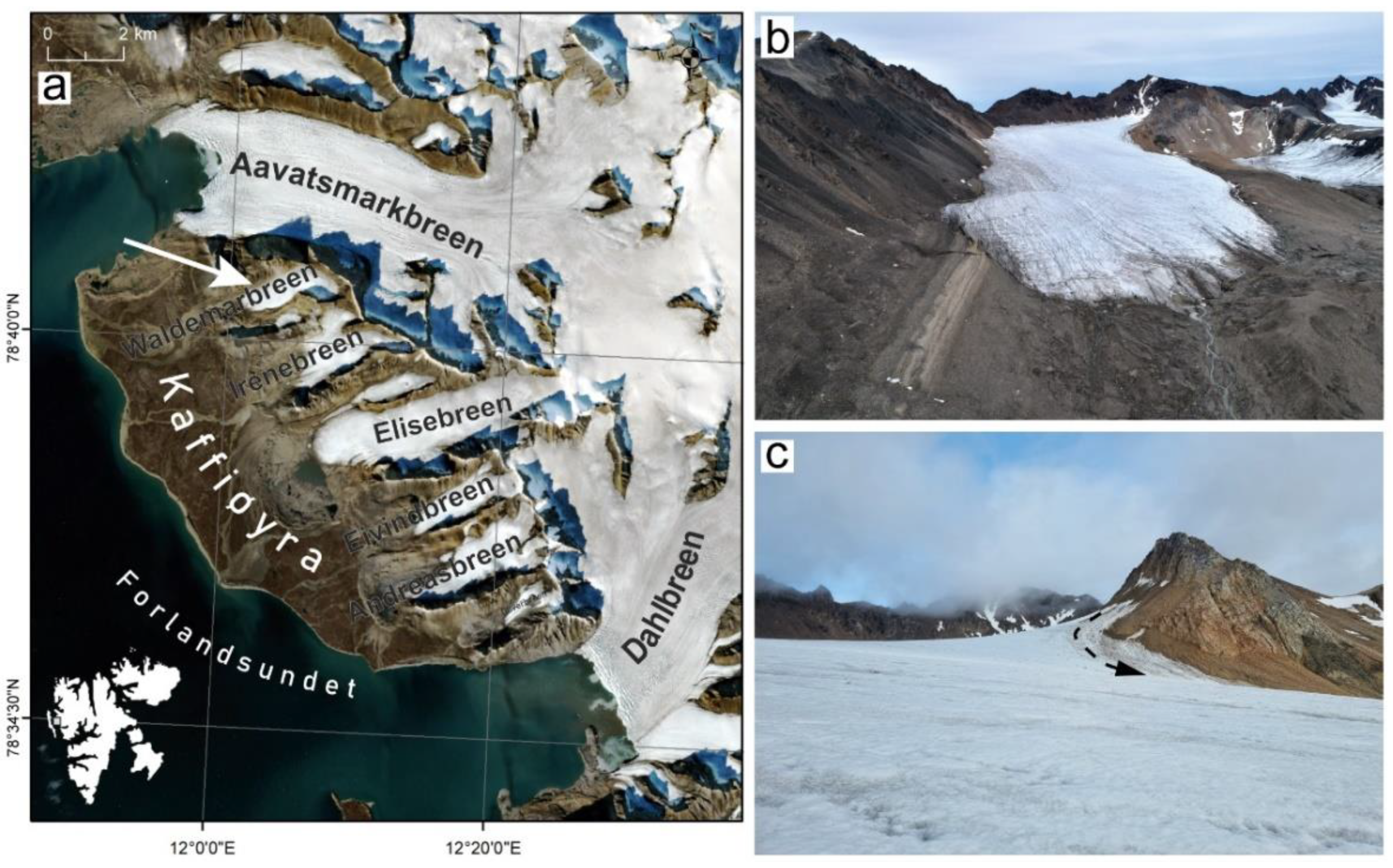
2. Study Area
3. Materials and Methods
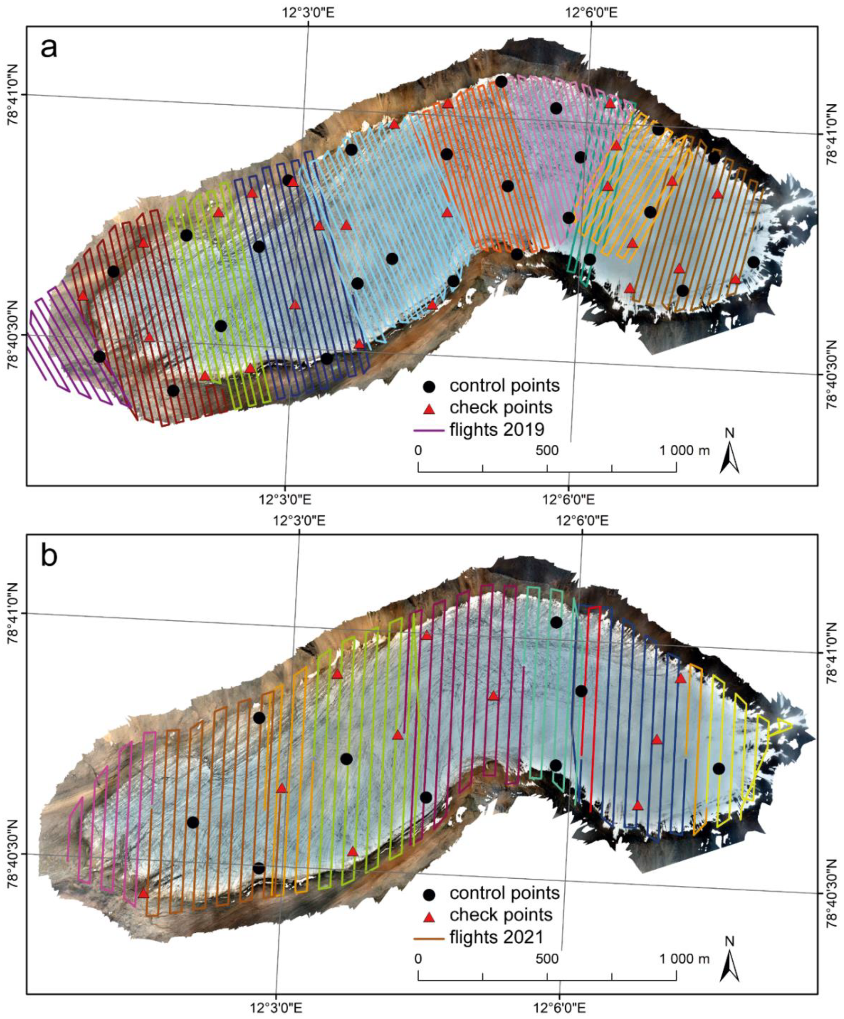
3.1. UAV Survey
3.2. GCPs and Flight Trajectory Corrections
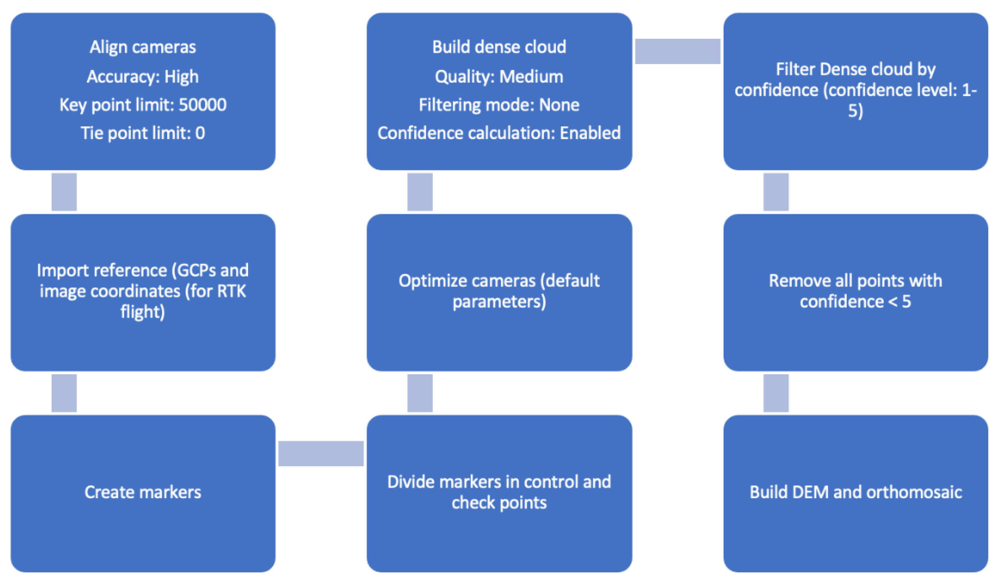
3.3. Orthophotos and Digital Surface Models from UAV Survey
3.4. Glacier Extent, Surface Elevation Change, and Mass Balance
3.5. Surface Velocity from UAV Products
4. Results
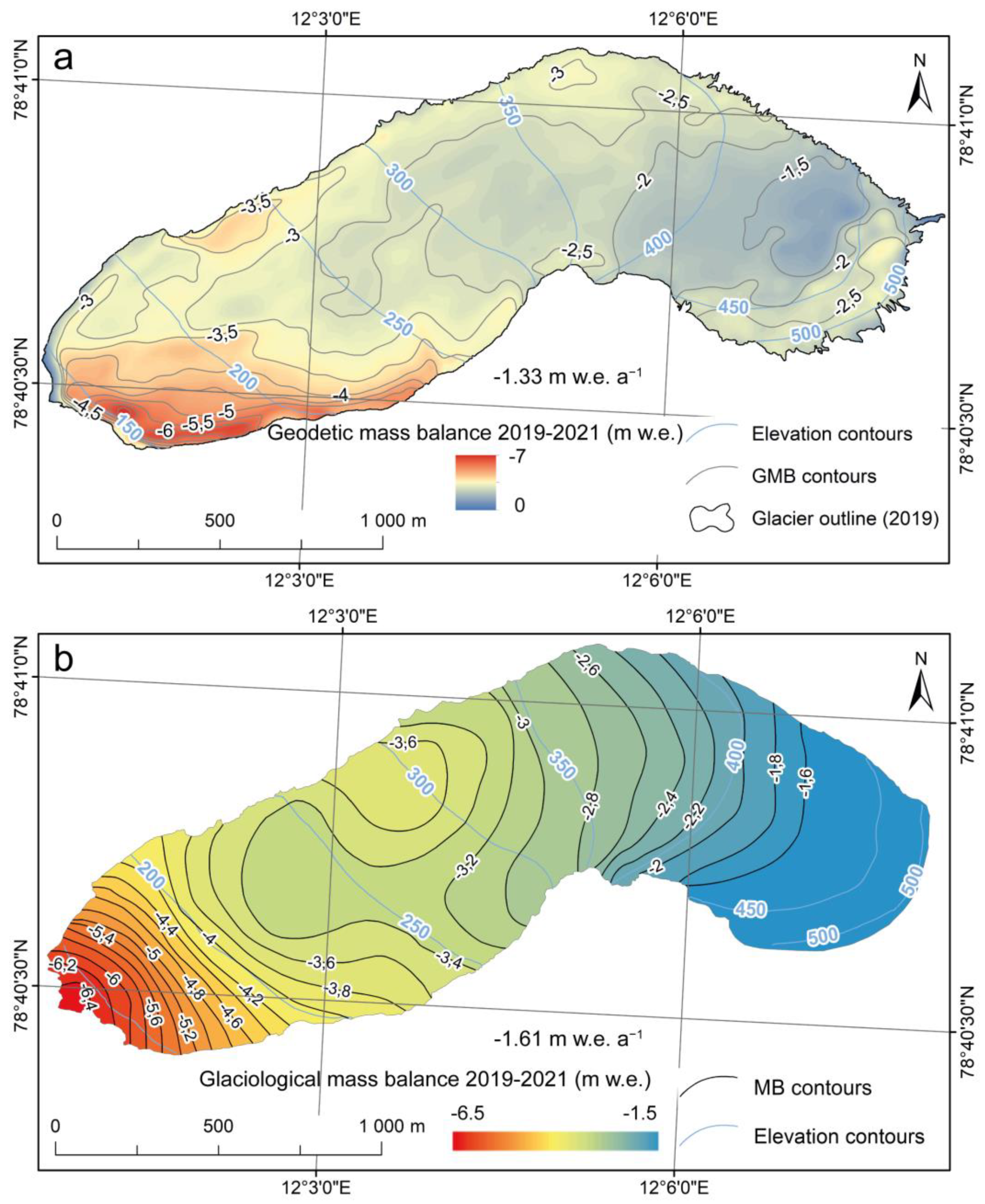
4.1. Glacier Surface Elevation Change and Geodetic Mass Balance
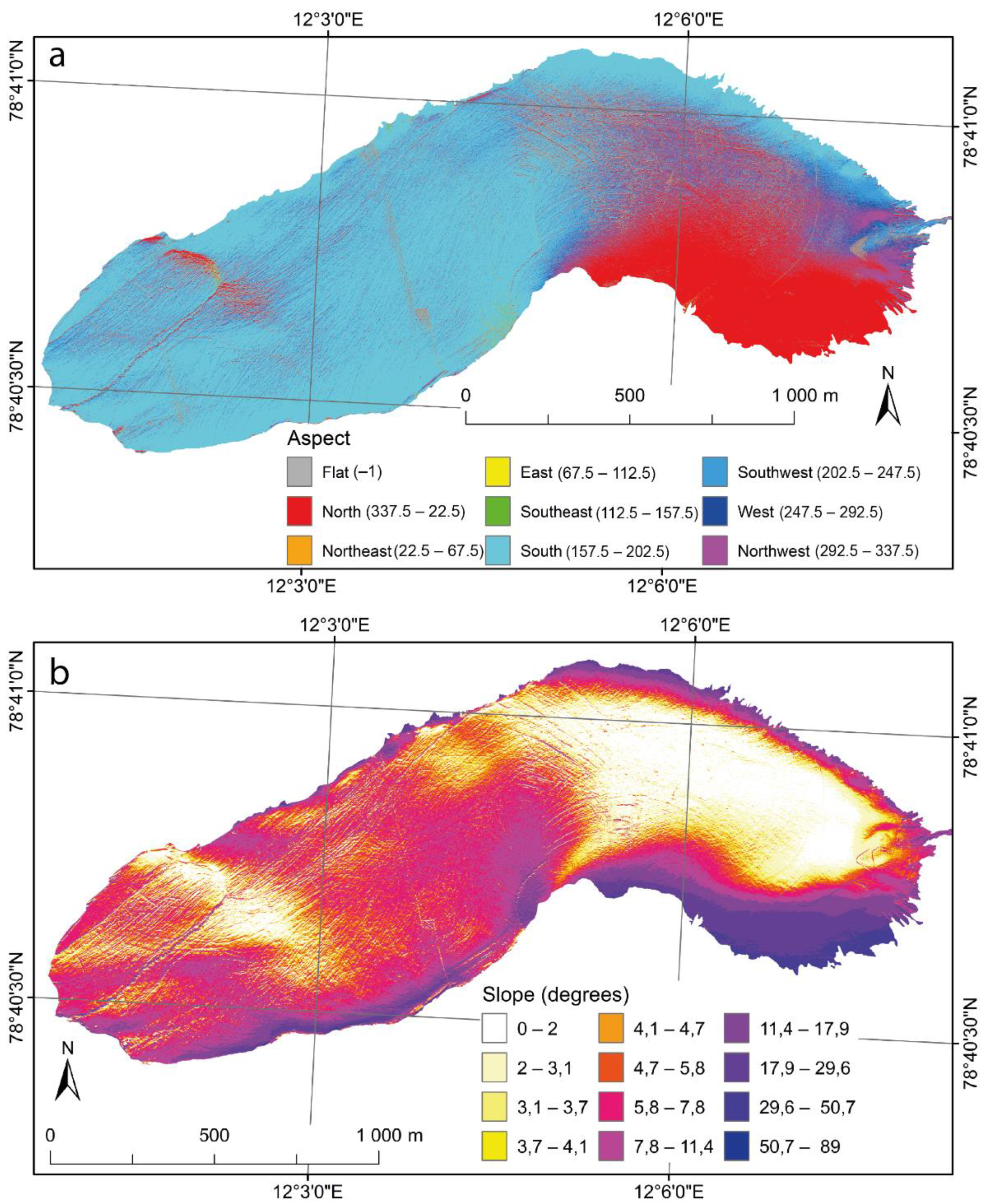
4.2. Glacier Surface Characteristics
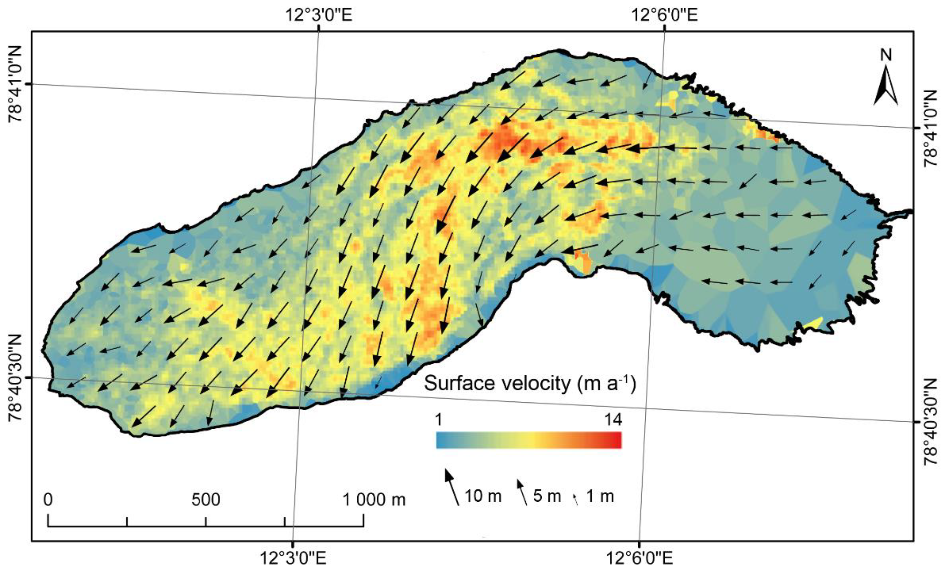
4.3. Glacier Surface Velocity
5. Discussion
5.1. Accuracy and Prospects of RTK UAV Surveys
5.2. Compression of Direct Glaciological and Geodetic Mass Balance
5.3. The Pattern of Surface Velocity of Waldemarbreen
5.4. UAV Surveys for Glacier Surface Velocity Estimation
6. Conclusions
Author Contributions
Funding
Institutional Review Board Statement
Data Availability Statement
Acknowledgments
Conflicts of Interest
References
- Cao, B.; Guan, W.; Li, K.; Pan, B.; Sun, X. High-Resolution Monitoring of Glacier Mass Balance and Dynamics with Unmanned Aerial Vehicles on the Ningchan No. 1 Glacier in the Qilian Mountains, China. Remote Sens. 2021, 13, 2735. [Google Scholar] [CrossRef]
- Nuth, C.; Moholdt, G.; Kohler, J.; Hagen, J.O.; Kääb, A. Svalbard glacier elevation changes and contribution to sea level rise. J. Geophys. Res. Earth Surf. 2010, 115, F01008. [Google Scholar] [CrossRef]
- Sobota, I.; Lankauf, K.R. Recession of Kaffiøyra region glaciers, Oscar II land, Svalbard. Bull. Geogr. Phys. Geogr. Ser. 2010, 3, 27–45. [Google Scholar] [CrossRef][Green Version]
- Sobota, I.; Nowak, M.; Weckwerth, P. Long-term changes of glaciers in north-western Spitsbergen. Glob. Planet Change 2016, 144, 182–197. [Google Scholar] [CrossRef]
- Andreassen, L.M.; Elvehøy, H.; Kjøllmoen, B.; Belart, J.M.C. Glacier change in Norway since the 1960s—An overview of mass balance, area, length and surface elevation changes. J. Glaciol. 2020, 66, 313–328. [Google Scholar] [CrossRef]
- Moholdt, G.; Kääb, A.; Messerli, A.; Nagy, T.; Winsvold, S.H. Monitoring Glaciers in Mainland Norway and Svalbard Using Sentinel; NVE Rapport 3–2021; Andreassen, L.M., Ed.; Norwegian Water Resources and Energy Directorate (NVE): Oslo, Norway, 2021.
- Schuler, T.V.; Kohler, J.; Elagina, N.; Hagen, J.O.M.; Hodson, A.J.; Jania, J.A.; Kääb, A.M.; Luks, B.; Małecki, J.; Moholdt, G.; et al. Reconciling Svalbard Glacier Mass Balance. Front. Earth Sci. 2020, 8, 156. [Google Scholar] [CrossRef]
- WGMS. Global Glacier Change Bulletin No. 3 (2016–2017); 2020, Updated, and Earlier Reports; ISC(WDS)/IUGG(IACS)/UNEP/UNESCO/WMO; Zemp, M., Gärtner-Roer, I., Nussbaumer, S.U., Bannwart, J., Rastner, P., Paul, F., Hoelzle, M., Eds.; World Glacier Monitoring Service: Zurich, Switzerland, 2020. [Google Scholar]
- IPCC. Climate Change 2021: The Physical Science Basis. Contribution of Working Group I to the Sixth Assessment Report of the Intergovernmental Panel on Climate Change; Masson-Delmotte, V., Zhai, P., Pirani, A., Connors, S.L., Péan, C., Berger, S., Caud, N., Chen, Y., Goldfarb, L., Gomis, M.I., et al., Eds.; Cambridge University Press: Cambridge, UK, 2021. [Google Scholar]
- Radić, V.; Hock, R. Regionally differentiated contribution of mountain glaciers and ice caps to future sea-level rise. Nat. Geosci. 2011, 4, 91–94. [Google Scholar] [CrossRef]
- Fischer, M.; Huss, M.; Hoelzle, M. Surface elevation and mass changes of all Swiss glaciers 1980–2010. Cryosphere 2015, 9, 525–540. [Google Scholar] [CrossRef]
- Bash, E.A.; Moorman, B.J.; Gunther, A. Detecting Short-Term Surface Melt on an Arctic Glacier Using UAV Surveys. Remote Sens. 2018, 10, 1547. [Google Scholar] [CrossRef]
- Rees, W.G. Remote Sensing of Snow and Ice, 1st ed.; CRC Press: Boca Raton, FL, USA, 2006. [Google Scholar]
- Pellikka, P.; Rees, W.G. Remote Sensing of Glaciers. Techniques for Topographic, Spatial and Thematic Mapping of Glaciers; Taylor & Francis Group: London, UK, 2009. [Google Scholar]
- Ulrich, V.; Williams, J.G.; Zahs, V.; Anders, K.; Hecht, S.; Höfle, B. Measurement of rock glacier surface change over different timescales using terrestrial laser scanning point clouds. Earth Surf. Dyn. 2021, 9, 19–28. [Google Scholar] [CrossRef]
- Lamsters, K.; Karušs, J.; Rečs, A.; Bērziņš, D. Detailed subglacial topography and drumlins at the marginal zone of Múlajökull outlet glacier, central Iceland: Evidence from low frequency GPR data. Polar Sci. 2016, 10, 470–475. [Google Scholar] [CrossRef]
- Ewertowski, M.W.; Tomczyk, A.M.; Evans, D.J.A.; Roberts, D.H.; Ewertowski, M.W. Operational Framework for Rapid, Very-high Resolution Mapping of Glacial Geomorphology Using Low-cost Unmanned Aerial Vehicles and Structure-from-Motion Approach. Remote Sens. 2019, 11, 65. [Google Scholar] [CrossRef]
- Eldhuset, K.; Andersen, P.H.; Hauge, S.; Isaksson, E.; Weydahl, D.J. ERS tandem InSAR processing for DEM generation, glacier motion estimation and coherence analysis on Svalbard. Int. J. Remote Sens. 2003, 24, 1415–1437. [Google Scholar] [CrossRef]
- Gourmelen, N.; Kim, S.W.; Shepherd, A.; Park, J.W.; Sundal, A.V.; Björnsson, H.; Pálsson, F. Ice velocity determined using conventional and multiple-aperture InSAR. Earth Planet. Sci. Lett. 2011, 307, 156–160. [Google Scholar] [CrossRef]
- Rosenau, R.; Scheinert, M.; Dietrich, R. A processing system to monitor Greenland outlet glacier velocity variations at decadal and seasonal time scales utilizing the Landsat imagery. Remote Sens. Environ. 2015, 169, 1–19. [Google Scholar] [CrossRef]
- Altena, B.; Scambos, T.; Fahnestock, M.; Kääb, A. Extracting recent short-term glacier velocity evolution over southern Alaska and the Yukon from a large collection of Landsat data. Cryosphere 2019, 13, 795–814. [Google Scholar] [CrossRef]
- Bingham, R.G.; Nienow, P.W.; Sharp, M.J. Intra-annual and intra-seasonal flow dynamics of a High Arctic polythermal valley glacier. Ann. Glaciol. 2003, 37, 181–188. [Google Scholar] [CrossRef]
- Copland, L.; Sharp, M.J.; Nienow, P.W. Links between short-term velocity variations and the subglacial hydrology of a predominantly cold polythermal glacier. J. Glaciol. 2003, 49, 337–348. [Google Scholar] [CrossRef]
- Frezzotti, M.; Capra, A.; Vittuari, L. Comparison between glacier ice velocities inferred from GPS and sequential satellite images. Ann. Glaciol. 1998, 27, 54–60. [Google Scholar] [CrossRef]
- Manson, R.; Coleman, R.; Morgan, P.; King, M. Ice velocities of the Lambert Glacier from static GPS observations. EPS 2000, 52, 1031–1036. [Google Scholar] [CrossRef]
- Hartl, L.; Fischer, A.; Stocker-Waldhuber, M.; Abermann, J. Recent speed-up of an alpine rock glacier: An updated chronology of the kinematics of outer hochebenkar rock glacier based on geodetic measurements. Geogr Ann. A 2016, 98, 129–141. [Google Scholar] [CrossRef]
- Rees, W.G.; Arnold, N.S. Mass balance and dynamics of a valley glacier measured by high-resolution LiDAR. Polar Rec. 2007, 43, 311–319. [Google Scholar] [CrossRef]
- Telling, J.W.; Glennie, C.; Fountain, A.G.; Finnegan, D.C. Analyzing glacier surface motion using LiDAR data. Remote Sens. 2017, 9, 283. [Google Scholar] [CrossRef]
- Bodin, X.; Thibert, E.; Sanchez, O.; Rabatel, A.; Jaillet, S. Multi-annual kinematics of an active rock glacier quantified from very high-resolution DEMs: An application-case in the French Alps. Remote Sens. 2018, 10, 547. [Google Scholar] [CrossRef]
- Chudley, T.R.; Christoffersen, P.; Doyle, S.H.; Abellan, A.; Snooke, N. High-accuracy UAV photogrammetry of ice sheet dynamics with no ground control. Cryosphere 2019, 13, 955–968. [Google Scholar] [CrossRef]
- Karušs, J.; Lamsters, K.; Ješkins, J.; Sobota, I.; Džeriņš, P. UAV and GPR Data Integration in Glacier Geometry Reconstruction: A Case Study from Irenebreen, Svalbard. Remote Sens. 2022, 14, 456. [Google Scholar] [CrossRef]
- Karušs, J.; Lamsters, K.; Sobota, I.; Ješkins, J.; Džeriņš, P.; Hodson, A. Drainage system and thermal structure of a High Arctic polythermal glacier: Waldemarbreen, western Svalbard. J. Glaciol. 2021, 1–14. [Google Scholar] [CrossRef]
- Karušs, J.; Lamsters, K.; Chernov, A.; Krievāns, M.; Ješkins, J. Subglacial topography and thickness of ice caps on the Argentine Islands. Antarct. Sci. 2019, 31, 332–344. [Google Scholar] [CrossRef]
- Lamsters, K.; Karušs, J.; Krievāns, M.; Ješkins, J. High-resolution orthophoto map and digital surface models of the largest Argentine Islands (the Antarctic) from unmanned aerial vehicle photogrammetry. J. Maps 2020, 16, 335–347. [Google Scholar] [CrossRef]
- Lamsters, K.; Karušs, J.; Krievāns, M.; Ješkins, J. The thermal structure, subglacial topography and surface structures of the NE outlet of Eyjabakkajökull, east Iceland. Polar Sci. 2020, 26, 100566. [Google Scholar] [CrossRef]
- Lamsters, K.; Karušs, J.; Krievāns, M.; Ješkins, J. High-Resolution Surface and Bed Topography Mapping of Russell Glacier (SW Greenland) Using UAV and GPR. ISPRS Ann. Photogramm. Remote Sens. Spat. Inf. Sci. 2020, 2, 757–763. [Google Scholar] [CrossRef]
- Lamsters, K.; Karušs, J.; Krievans, M.; Ješkins, J. Application of Unmanned Aerial Vehicles for Glacier Research in the Arctic and Antarctic. In Environment. Technologies. Resources, Proceedings of the 12th International Scientific and Practical Conference, Rezekne, Latvia, 20–22 June 2019; Rezekne Academy of Technologies: Rezekne, Latvia, 2019; Volume 1, pp. 131–135. [Google Scholar]
- Paul, F.; Bolch, T.; Kääb, A.; Nagler, T.; Nuth, C.; Scharrer, K.; Shepherd, A.; Strozzi, T.; Ticconi, F.; Bhambri, R.; et al. The glaciers climate change initiative: Methods for creating glacier area, elevation change and velocity products. Remote Sens. Environ. 2015, 162, 408–426. [Google Scholar] [CrossRef]
- Błaszczyk, M.; Ignatiuk, D.; Grabiec, M.; Kolondra, L.; Laska, M.; Decaux, L.; Jania, J.; Berthier, E.; Luks, B.; Barzycka, B.; et al. Quality assessment and glaciological applications of digital elevation models derived from space-borne and aerial images over two tidewater glaciers of southern Spitsbergen. Remote Sens. 2019, 11, 1121. [Google Scholar] [CrossRef]
- Noh, M.-J.; Howat, I.M. The Surface Extraction from TIN based Search-space Minimization (SETSM) algorithm. ISPRS J. Photogramm. Remote Sens. 2017, 129, 55–76. [Google Scholar] [CrossRef]
- Noh, M.-J.; Howat, I.M. Automated stereo-photogrammetric DEM generation at high latitudes: Surface Extraction with TIN-based Search-space Minimization (SETSM) validation and demonstration over glaciated regions. GISci. Remote Sens. 2015, 52, 198–217. [Google Scholar] [CrossRef]
- Sobota, I.; Weckwerth, P.; Nowak, M. Surge dynamics of Aavatsmarkbreen, Svalbard, inferred from the geomorphological record. Boreas 2016, 45, 360–376. [Google Scholar] [CrossRef]
- Śledź, S.; Ewertowski, M.; Piekarczyk, J. Applications of unmanned aerial vehicle (UAV) surveys and Structure from Motion photogrammetry in glacial and periglacial geomorphology. Geomorphology 2021, 378, 107620. [Google Scholar] [CrossRef]
- Kraaijenbrink, P.; Meijer, S.W.; Shea, J.M.; Pellicciotti, F.; de Jong, S.M.; Immerzeel, W.W. Seasonal surface velocities of a Himalayan glacier derived by automated correlation of unmanned aerial vehicle imagery. Ann. Glaciol. 2016, 57, 103–113. [Google Scholar] [CrossRef]
- Rossini, M.; di Mauro, B.; Garzonio, R.; Baccolo, G.; Cavallini, G.; Mattavelli, M.; de Amicis, M.; Colombo, R. Rapid melting dynamics of an alpine glacier with repeated UAV photogrammetry. Geomorphology 2018, 304, 159–172. [Google Scholar] [CrossRef]
- Xue, Y.; Jing, Z.; Kang, S.; He, X.; Li, C. Combining UAV and Landsat data to assess glacier changes on the central Tibetan Plateau. J. Glaciol. 2021, 67, 1–13. [Google Scholar] [CrossRef]
- Wang, P.; Li, H.; Li, Z.; Liu, Y.; Xu, C.; Mu, J.; Zhang, H. Seasonal Surface Change of Urumqi Glacier No. 1, Eastern Tien Shan, China, Revealed by Repeated High-Resolution UAV Photogrammetry. Remote Sens. 2021, 13, 3398. [Google Scholar] [CrossRef]
- Bhardwaj, A.; Sam, L.; Martín-Torres, F.J.; Kumar, R. UAVs as remote sensing platform in glaciology: Present applications and future prospects. Remote Sens. Environ. 2016, 175, 196–204. [Google Scholar] [CrossRef]
- Peppa, M.V.; Hall, J.; Goodyear, J.; Mills, J.P. Photogrammetric assessment and comparison of DJI Phantom 4 pro and phantom 4 RTK small unmanned aircraft systems. Int. Arch. Photogramm. Remote Sens. Spat. Inf. Sci. 2019, XLII-2/W13, 503–509. [Google Scholar] [CrossRef]
- Štroner, M.; Urban, R.; Reindl, T.; Seidl, J.; Brouček, J. Evaluation of the georeferencing accuracy of a photogrammetric model using a quadrocopter with onboard GNSS RTK. J. Sens. 2020, 20, 2318. [Google Scholar] [CrossRef]
- Taddia, Y.; Stecchi, F.; Pellegrinelli, A. Coastal mapping using DJI Phantom 4 RTK in post-processing kinematic mode. Drones 2020, 4, 9. [Google Scholar] [CrossRef]
- Sobota, I. Ablation of the Waldemar Glacier in the summer seasons 1996, 1997 and 1998. Pol. Polar Stud. 1999, 26, 257–274. [Google Scholar]
- Sobota, I. Selected methods in mass balance estimation of Waldemar Glacier, Spitsbergen. Pol. Polar. Res. 2007, 28, 249–268. [Google Scholar]
- Sobota, I. The near-surface ice thermal structure of the Waldemarbreen, Svalbard. Polar Res. 2009, 30, 317–338. [Google Scholar] [CrossRef]
- Sobota, I. Icings and their role as an important element of the cryosphere in High Arctic glacier forefields. Bull. Geogr. Phys. Geogr. Ser. 2016, 10, 81–93. [Google Scholar] [CrossRef]
- Sobota, I. Selected problems of snow accumulation on glaciers during long-term studies in north-western Spitsbergen, Svalbard. Geogr. Ann. A 2017, 99, 1–16. [Google Scholar] [CrossRef]
- Sobota, I. (Ed.) Atlas of Changes in the Glaciers of Kaffiøyra (Svalbard, the Arctic), 1st ed.; Scientific Publishers of the Nicolaus Copernicus University: Toruń, Poland, 2021. [Google Scholar]
- Sobota, I. Changes in dynamics and runoff from the High Arctic glacial catchment of Waldemarbreen, Svalbard. Geomorphology 2014, 212, 16–27. [Google Scholar] [CrossRef]
- Kejna, M.; Sobota, I. Meteorological conditions on Kaffiøyra (NW Spitsbergen) in 2013–2017 and their connection with atmospheric circulation and sea ice extent. Pol. Polar Res. 2019, 40, 175–204. [Google Scholar]
- Porter, C.; Morin, P.; Howat, I.; Noh, M.-J.; Bates, B.; Peterman, K.; Keesey, S.; Schlenk, M.; Gardiner, J.; Tomko, K.; et al. ArcticDEM; Harvard Dataverse, V1: Cambridge, MA, USA, 2018. [Google Scholar]
- James, M.R.; Chandler, J.H.; Eltner, A.; Fraser, C.; Miller, P.E.; Mills, J.P.; Noble, T.; Robson, S.; Lane, S.N. Guidelines on the use of structure-from-motion photogrammetry in geomorphic research. Earth Surf. Process. Landf. 2019, 44, 2081–2084. [Google Scholar] [CrossRef]
- Sobota, I.; Weckwerth, P.; Grajewski, T. Rain-on-Snow (ROS) events and their relations to snowpack and ice layer changes on small glaciers in Svalbard, the high Arctic. J. Hydrol. 2020, 590, 1–11. [Google Scholar] [CrossRef]
- Østrem, G.; Brugman, M. Glacier Mass-Balance Measurements: A Manual for Field and Office Work, 1st ed.; National Hydrology Research Institute: Saskatoon, SK, Canada, 1991. [Google Scholar]
- Cogley, J.G.; Hock, R.; Rasmussen, L.A.; Arendt, A.A.; Bauder, A.; Braithwaite, R.J.; Jansson, P.; Kaser, G.; Moller, M.; Nicholson, L.; et al. Glossary of Glacier Mass Balance and Related Terms; IHP-VII Technical Documents in Hydrology No. 86; IACS Contribution No. 2; UNESCO-IHP: Paris, France, 2011. [Google Scholar]
- Gardner, A.S.; Moholdt, G.; Scambos, T.; Fahnstock, M.; Ligtenberg, S.; van den Broeke, M.; Nilsson, J. Increased West Antarctic and unchanged East Antarctic ice discharge over the last 7 years. Cryosphere 2018, 12, 521–547. [Google Scholar] [CrossRef]
- Zheng, W.; Durkin, W.J.; Melkonian, A.K.; Pritchard, M.E. Cryosphere and Remote Sensing Toolkit (CARST) v2.0.0a1 (Version v2.0.0a1); Zenodo: Meyrin, Switzerland, 2021. [Google Scholar] [CrossRef]
- Van Wyk de Vries, M.; Wickert, A.D. Glacier Image Velocimetry: An open-source toolbox for easy and rapid calculation of high-resolution glacier velocity fields. Cryosphere 2021, 15, 2115–2132. [Google Scholar] [CrossRef]
- Scambos, T.A.; Dutkiewicz, M.J.; Wilson, J.C.; Bindschadler, R.A. Application of image cross-correlation to the measurement of glacier velocity using satellite image data. Remote Sens. Environ. 1992, 42, 177–186. [Google Scholar] [CrossRef]
- Cusicanqui, D.; Rabatel, A.; Vincent, C.; Bodin, X.; Thibert, E.; Francou, B. Interpretation of volume and flux changes of the Laurichard rock glacier between 1952 and 2019, French Alps. J. Geophys. Res. Earth Surf. 2021, 126, e2021JF006161. [Google Scholar] [CrossRef]
- Hormes, A.; Adams, M.; Amabile, A.S.; Blauensteiner, F.; Demmler, C.; Fey, C.; Ostermann, M.; Rechberger, C.; Sausgruber, T.; Vecchiotti, F.; et al. Innovative methods to monitor rock and mountain slope deformation. Geomech. Tunn. 2020, 13, 88–102. [Google Scholar] [CrossRef]
- Fleischer, F.; Haas, F.; Piermattei, L.; Pfeiffer, M.; Heckmann, T.; Altmann, M.; Rom, J.; Stark, M.; Wimmer, M.H.; Pfeifer, N.; et al. Multi-decadal (1953–2017) rock glacier kinematics analysed by high-resolution topographic data in the upper Kaunertal, Austria. Cryosphere 2021, 15, 5345–5369. [Google Scholar] [CrossRef]
- Fey, C.; Krainer, K. Analyses of UAV and GNSS based flow velocity variations of the rock glacier Lazaun (Ötztal Alps, South Tyrol, Italy). Geomorphology 2020, 365, 107261. [Google Scholar] [CrossRef]
- Dabove, P.; Linty, N.; Dovis, F. Analysis of multi-constellation GNSS PPP solutions under phase scintillations at high latitudes. Appl. Geomat. 2020, 12, 45–52. [Google Scholar] [CrossRef]
- Cox, L.H.; March, R.S. Comparison of geodetic and glaciological mass-balance techniques, Gulkana Glacier, Alaska, USA. J. Glaciol. 2004, 50, 363–370. [Google Scholar] [CrossRef]
- Fischer, A. Comparison of direct and GMBs on a multi-annual time scale. Cryosphere Discuss. 2010, 4, 1151–1194. [Google Scholar]
- Cogley, J.G. Geodetic and direct mass-balance measurements: Comparison and joint analysis. Ann. Glaciol. 2009, 50, 96–100. [Google Scholar] [CrossRef]
- Wagnon, P.; Brun, F.; Khadka, A.; Berthier, E.; Shrestha, D.; Vincent, C.; Arnaud, Y.; Six, D.; Dehecq, A.; Ménégoz, M.; et al. Reanalysing the 2007–19 glaciological mass-balance series of Mera Glacier, Nepal, Central Himalaya, using GMB. J. Glaciol. 2021, 67, 117–125. [Google Scholar] [CrossRef]
- Melkonian, A.K.; Willis, M.J.; Pritchard, M.E. Satellite-derived volume loss rates and glacier speeds for the Juneau Icefield, Alaska. J. Glaciol. 2014, 60, 743–760. [Google Scholar] [CrossRef]
- Kääb, A.; Vollmer, M. Surface geometry, thickness changes and flow fields on creeping mountain permafrost: Automatic extraction by digital image analysis. Permafr. Periglac. Process. 2000, 11, 315–326. [Google Scholar] [CrossRef]
- Jouvet, G.; Weidmann, Y.; van Dongen, E.; Lüthi, M.P.; Vieli, A.; Ryan, J.C. High-endurance UAV for monitoring calving glaciers: Application to the Inglefield Bredning and Eqip Sermia, Greenland. Front. Earth Sci. 2019, 7, 206. [Google Scholar] [CrossRef]
- James, M.R.; Robson, S.; d’Oleire-Oltmanns, S.; Niethammer, U. Optimising UAV topographic surveys processed with structure-from-motion: Ground control quality, quantity and bundle adjustment. Geomorphology 2017, 280, 51–66. [Google Scholar] [CrossRef]
- Karimi, N.; Sheshangosht, S.; Roozbahani, R. High-resolution monitoring of debris-covered glacier mass budget and flow velocity using repeated UAV photogrammetry in Iran. Geomorphology 2021, 389, 107855. [Google Scholar] [CrossRef]
- Lague, D.; Brodu, N.; Leroux, J. Accurate 3D comparison of complex topography with terrestrial laser scanner: Application to the Rangitikei canyon (NZ). ISPRS J. Photogram. Remote Sens. 2013, 82, 10–26. [Google Scholar] [CrossRef]


| Parameter | DJI Phantom 4 Pro V2.0 | DJI Phantom 4 RTK |
|---|---|---|
| Sensor | 1″ CMOS sensor | 1″ CMOS sensor |
| Sensor resolution | 20 Mpx | 20 Mpx |
| Lens | 8.8mm/24mm f/2.8–f/11 | 8.8mm/24mm f/2.8–f/11 |
| Shutter | Mechanical and electronic | Mechanical and Electronic |
| Satellite positioning system | GPS/GLONASS | GPS/GLONASS/Galileo/BeiDou |
| RTK | - | + |
| Position accuracy | ~1.5m | ~0.015m with RTK |
| Statistics | 2019 Survey | 2021 Survey |
|---|---|---|
| Number of GCPs | 49 | 19 |
| Average GCP RMSE (control points) | 0.045m(horizontal)/0.081m(vertical)/0.104m (total) | 0.009m(horizontal)/0.02m(vertical)/0.024m(total) |
| Average GCP RMSE (check points) | 0.095m(horizontal)/0.228m(vertical)/0.273m(total) | 0.089m(horizontal)/0.365m(vertical)/0.387m (total) |
| Number of control points | 24 | 9 |
| Number of checkpoints | 25 | 10 |
| Number of images | 2920 | 4286 |
| RMS reprojection error | 0.196 (0.678 pix) | 0.164 (0.9377 pix) |
Publisher’s Note: MDPI stays neutral with regard to jurisdictional claims in published maps and institutional affiliations. |
© 2022 by the authors. Licensee MDPI, Basel, Switzerland. This article is an open access article distributed under the terms and conditions of the Creative Commons Attribution (CC BY) license (https://creativecommons.org/licenses/by/4.0/).
Share and Cite
Lamsters, K.; Ješkins, J.; Sobota, I.; Karušs, J.; Džeriņš, P. Surface Characteristics, Elevation Change, and Velocity of High-Arctic Valley Glacier from Repeated High-Resolution UAV Photogrammetry. Remote Sens. 2022, 14, 1029. https://doi.org/10.3390/rs14041029
Lamsters K, Ješkins J, Sobota I, Karušs J, Džeriņš P. Surface Characteristics, Elevation Change, and Velocity of High-Arctic Valley Glacier from Repeated High-Resolution UAV Photogrammetry. Remote Sensing. 2022; 14(4):1029. https://doi.org/10.3390/rs14041029
Chicago/Turabian StyleLamsters, Kristaps, Jurijs Ješkins, Ireneusz Sobota, Jānis Karušs, and Pēteris Džeriņš. 2022. "Surface Characteristics, Elevation Change, and Velocity of High-Arctic Valley Glacier from Repeated High-Resolution UAV Photogrammetry" Remote Sensing 14, no. 4: 1029. https://doi.org/10.3390/rs14041029
APA StyleLamsters, K., Ješkins, J., Sobota, I., Karušs, J., & Džeriņš, P. (2022). Surface Characteristics, Elevation Change, and Velocity of High-Arctic Valley Glacier from Repeated High-Resolution UAV Photogrammetry. Remote Sensing, 14(4), 1029. https://doi.org/10.3390/rs14041029