Article

In Situ Measuring Stem Diameters of Maize Crops with a High-Throughput Phenotyping Robot

1
College of Mechanical and Electronic Engineering, Northwest A&F University, Xianyang 712100, China
2
Intelligent Equipment Research Center, Beijing Academy of Agriculture and Forestry Sciences, Beijing 100097, China
3
College of Engineering and Technology, Southwest University, Chongqing 400715, China
4
Academy of Artificial Intelligence, Beijing Institute of Petrochemical Technology, Beijing 102617, China
5
National Engineering Research Center for Information Technology in Agriculture, Beijing 100097, China
*
Author to whom correspondence should be addressed.
These authors contributed equally to this work.
Remote Sens. 2022, 14(4), 1030; https://doi.org/10.3390/rs14041030
Submission received: 14 December 2021 / Revised: 9 February 2022 / Accepted: 17 February 2022 / Published: 21 February 2022
(This article belongs to the Special Issue Imaging for Plant Phenotyping)

Abstract

:
Robotic High-Throughput Phenotyping (HTP) technology has been a powerful tool for selecting high-quality crop varieties among large quantities of traits. Due to the advantages of multi-view observation and high accuracy, ground HTP robots have been widely studied in recent years. In this paper, we study an ultra-narrow wheeled robot equipped with RGB-D cameras for inter-row maize HTP. The challenges of the narrow operating space, intensive light changes, and messy cross-leaf interference in rows of maize crops are considered. An in situ and inter-row stem diameter measurement method for HTP robots is proposed. To this end, we first introduce the stem diameter measurement pipeline, in which a convolutional neural network is employed to detect stems, and the point cloud is analyzed to estimate the stem diameters. Second, we present a clustering strategy based on DBSCAN for extracting stem point clouds under the condition that the stem is shaded by dense leaves. Third, we present a point cloud filling strategy to fill the stem region with missing depth values due to the occlusion by other organs. Finally, we employ convex hull and plane projection of the point cloud to estimate the stem diameters. The results show that the R2 and RMSE of stem diameter measurement are up to 0.72 and 2.95 mm, demonstrating its effectiveness.

Graphical Abstract

1. Introduction

Agricultural production is undergoing the ever-increasing challenges of global climate change, natural disasters, and population growth. The global population is expected to reach 10 billion [1,2], meaning that a 70% increment of crop yields has to be achieved over the next 30 years to meet the growing demand for food [3,4]. To increase the crop yields, molecular/genetic technology has been utilized in the breeding process [5]. However, the manual phenotypic screening in breeding is usually high-cost, time-consuming, and laborious, leading to a bottleneck in the further development of breeding technology [6,7]. The robotic HTP technique provides abundant phenotypic information in an automated and effective way and considerably eases the manual workload of breeders to select high-yield varieties from a large amount of samples [8]. Consequently, robotic HTP has been one of the most attractive topics in agriculture [9].
Maize, one of the main food and economic crops, has been the focus of many breeders in cultivating new varieties. High-throughput phenotyping of maize crops is a critical step to improve the yield. Particularly, the stem diameter of maize crops is an important index to measure the lodging resistance [10], which requires the HTP robots to collect phenotypic data of stems through inter-row shuttling. Unfortunately, the inter-row environment is narrow, the lighting varies, and leaf-occlusion clutter is present. Furthermore, the depth noise or error of three-dimensional (3D) sensors used to collect phenotypic data has a negative effect on the estimation accuracy of phenotypic parameters. Low-quality depth information cannot completely represent the 3D structure of crops [11,12]. Determining how to overcome these difficulties to accurately estimate the stem diameter between crop rows is urgent and challenging.
In our work, we study a stem diameter measurement pipeline on a self-developed phenotyping platform equipped with an RGB-D camera and propose an HTP robot system from data acquisition to analyze phenotypic parameters and measure the maize stem diameters under complicated field conditions. The main contributions are summarized as follows:
  • A strategy of stem point cloud extraction is proposed to cope with the stems in the shade of dense leaves. This strategy solves the problem of extracting stem point clouds under canopy with narrow row spacing and cross-leaf occlusion;
  • A real-time measurement pipeline is proposed to estimate the stem diameters. In this pipeline, we present two novel stem diameter estimation approaches based on stem point cloud geometry. Our approaches can effectively reduce the influences of depth noise or error on the estimation results;
  • A post-processing approach is presented to fill the missing parts of the stem point clouds caused by the occlusion of dense adjacent leaves. This approach ensures the integrity of the stem point clouds obtained by RGB-D cameras in complex field scenarios and improves the accuracy of stem diameter estimation.
We hope that the study of stem diameter estimation for high-stem crops, such as maize, in real and complex field scenarios can accelerate the development of field phenotypic equipment and technology.

2. Related Works

2.1. HTP Platforms

Field-based HTP is a multi-scale crop observation technique based on phenotyping platforms equipped with multiple types of sensors [13]. Currently, the common phenotyping platforms can be roughly divided into three types: fixed, aerial, and mobile platforms [14]. Based on the inherent properties of these platforms, phenotyping parameters can be obtained at various scales, from organ level to plot level. Generally, the fixed platforms fitted with visual and laser sensors allow for high-accuracy monitoring of different crop organs with a 360° view [15,16]. However, they only obtain the phenotyping parameters of fixed plots. Aerial platforms, such as Unmanned Aerial vehicles (UAVs), enable rapid observation of crops at the plot level [17]. However, the sensing accuracy gradually decreases with increases in flight altitude [18,19]. Mobile platforms, especially mobile robots, are a new type of phenotyping platform that can travel freely in breeding fields. This high mobility gives them a unique ability: they can automatically obtain phenotypic parameters between narrow crop rows in different plots [20,21]. Therefore, the mobile robots used for phenotypic observation integrate the dual advantages of fixed and aerial platforms, which is significant for promoting the rapid development of phenomics [22].

2.2. HTP Robots

As an interdisciplinary subject of agronomy, computer science, and robotics, phenotyping technologies based on mobile robots equipped with various phenotyping sensors, named with HTP robots, have been widely reported [23,24,25,26]. The representative HTP robots come from some of the top research institutions, such as Carnegie Mellon University [27,28] and the University of Illinois at Urbana-Champaign [29,30]. Their HTP robots focus on crop row phenotyping of high-stem crops (maize, sorghum, and sugarcane, for example) by stereo cameras and/or depth cameras. Ref. [28] presented a deep–learning-based online pipeline for in situ sorghum stem detection and grasping. Ref. [29] developed a tracked HTP robot from design to field evaluation, and measured the stem height and width of energy sorghum based on their previous work. Ref. [30] described high-precision control and corn stand counting algorithms for an autonomous field robot. Additionally, Ref. [31] employed the “Phenomobile”, a phenotyping robot [32] equipped with 3D LIDAR to obtain the row spacing and plant height of a maize field. The highlight of this work is that the HTP robot could obtain parcel-level phenotyping parameters by moving along the side of a road in a breeding field, rather than traveling between crop rows.

2.3. Phenotyping Sensors

These advanced robots have exhibited excellent performance in terms of plant phenotyping, which benefits from phenotyping sensors used to perceive crop information. Color digital cameras, spectrometers (hyperspectral and multispectral), thermal infrared cameras, etc. are widely used on HTP robots [33]. In addition, some 3D sensors, stereo cameras, depth cameras, and LIDAR, can be used to obtain crop 3D data. Based on the sensing data, crops’ morphological and structural parameters can be extracted [34]. Although these sensors work well in phenotyping, they usually only capture a single type of data. For example, color digital cameras and LIDAR can only capture RGB images and 3D point clouds, respectively. Stereo cameras can calculate the depth values of observed targets from two RGB images with different perspectives, but they have heavy computation loads [35]. In recent years, RGB-D cameras have received sufficient attention in the application of HTP [36,37], because they can obtain color and depth images in the same frame at close range, which makes them a potential alternative to color cameras and LIDAR. In our work, we conduct phenotyping using a self-developed phenotyping platform equipped with an RGB-D camera.

2.4. Maize Phenotyping

Field-based maize phenotyping is difficult under natural growing conditions because of the disturbance of lighting conditions and crossover/shading of leaves from adjacent shoots that occurs in the later growth stages. Thus, many phenotyping studies have focused on the early growth stages, observing the maize canopy with top-view and relatively regular scenarios [38,39,40]. Ref. [39] proposed an approach to extract morphological and color-related phenotypes that uses an end–to–end segmentation network from top-view images at the seeding stage. Ref. [40] utilized image sequences obtained by UAV to reconstruct a 3D model of maize crops and estimated the leaf number, plant height, individual leaf area, etc. Ref. [38] developed a robot system composed of a four-degree robotic manipulator, a ToF camera, and a linear potentiometer, which used deep learning and conventional image processing to detect and grasp maize stems in a greenhouse. Admittedly, some exploratory studies have been carried out in real open fields, as mentioned in references [27,29]. Ref. [41] described a 3D reconstruction and point cloud processing pipeline of maize crops in the native environment, and realized the extraction of main parameters for individual plant phenotypic characteristics. However, some key technologies, such as feature recognition, phenotypic parameter extraction, and occlusion mentioned above, still need to be addressed in a better way. The maize yield is directly influenced by lodging tolerance. Related studies have shown that lodging can cause 80% yield losses, depending on the crop and field location [42]. The stem strength of crops is an important index of lodging tolerance. Herein, our research interests focus on the automatic measurement of maize stem diameters during the mature stage in the natural environment.

3. Materials and Methods
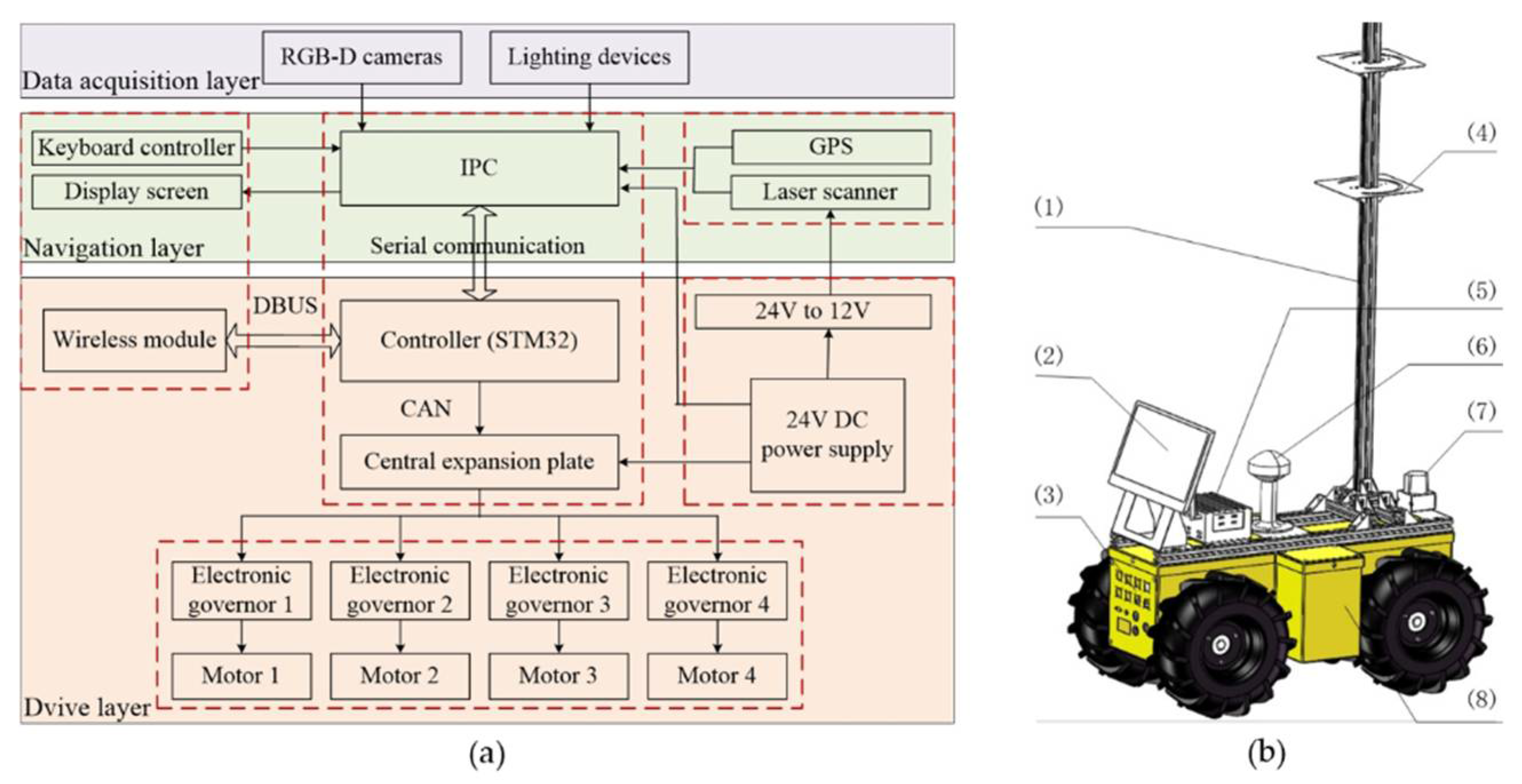
3.1. HTP Platform

Maize plants usually have row spacing of 0.5–0.8 m for most cultivation patterns of equal row spacing. To extract the phenotypic parameters automatically under these cultivation patterns, we developed an ultra-narrow phenotyping robot platform that can move between maize crop rows [43]. The mechanical dimensions of the platform are 0.80 m × 0.45 m × 0.40 m (length × width × height, not counting the height of the mast), with a mass of 40 kg. In addition, a retractable mast could be mounted on the robot platform. It is used to fix sensors to observe crop organs during any growth period of maize. The maximum height of the mast can reach 2.2 m.
The robot system adopted a distributed design. We divided it into three control units: driving module, navigation module, and phenotypic data acquisition module. The driving module was a wireless remote-control system and the navigation module was a control system based on an industrial personal computer (IPC). The bottom controller of the robot was an STM32 development board, which was used for the motion control of four electronic governors by connecting to a central expansion board. The four electronic governors were four deceleration motors connected to the wheel bearing. The navigation module used a Global Navigation Satellite System (GNSS) and a laser scanner to realize the mapping and navigation in the field based on Cartographer, a simultaneous localization and mapping (SLAM) algorithm. Notes that the navigation module was an integral part of our robot, but it was not the research focus of this paper. The data acquisition module consisted of an RGB-D camera and four lighting devices, which could ensure that the robot walking under the dense canopy could still capture sufficient 3D information of crops, even in poor lighting conditions. The robot software algorithms we developed were coded under Robot Operating System (ROS) based on Ubuntu 20.04. The schematic of our HTP robot platform is shown in Figure 1. The specifications and parameters of our robot are shown in Table 1.

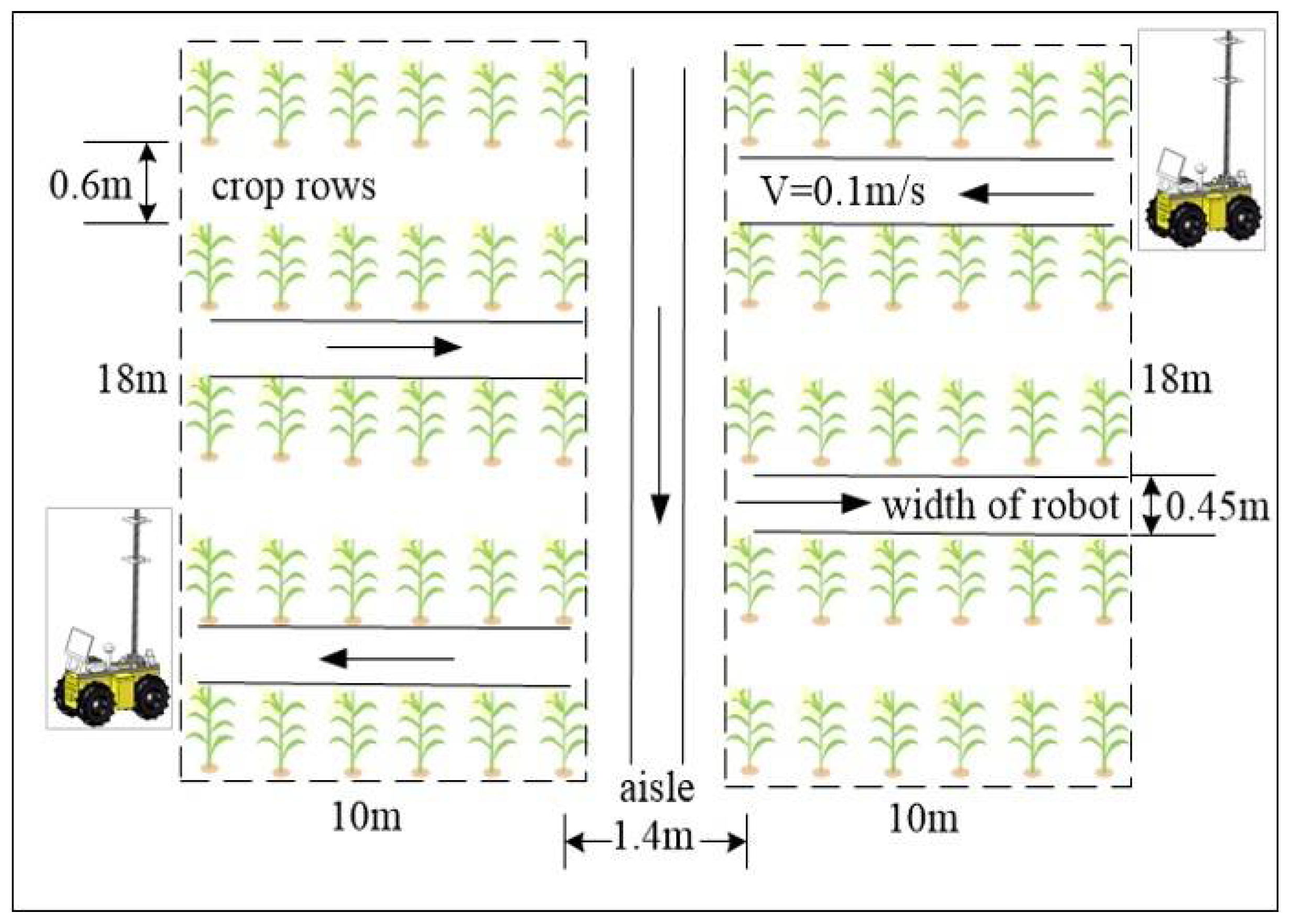
3.2. Field Data Collection

We conducted field experiments at the Beijing Academy of Agriculture and Forestry Sciences in August 2020. We selected a planting area of 18 × 22 m2 as the experimental area, which was composed of three parts: crops, crop rows, and aisles. Our robot could move freely through the crop rows and aisles in the teleoperation mode. Usually, the stem portion at the base of crops had a greater impact on the lodging resistance. To ensure that the sensor’s field of view covered the basal stem area as much as possible, we fixed the RGB-D camera (Intel® RealSense D435i) to a tray with a height of 0.5 m. Besides, due to the poor lighting conditions under dense crop canopies, we also installed four LED lighting devices on sensor trays. These LED lights were kept on as the robot worked between crop rows. To prevent the camera lens from being blocked by the messy maize leaves, we kept the camera lens facing opposite to the moving direction of the robot, which could reduce the contact frequency between the camera lens and the leaves. In this way, the RGB-D camera could capture the stems on either side of the crop rows.
The specific experimental scheme is shown in Figure 2. The aisle divided the experimental field into two areas of 10 × 18 m2. For each area, the crop row spacing was 0.6 m. The robot collected phenotypic data from 8 crop rows at a speed of 0.1 m/s. In addition, to enrich our data sets, we kept our robot moving in an aisle with a width of 1.4 m to collect phenotypic data for both sides of the crop areas. The arrows in Figure 2 show the route traveled by our robot.
During our experiments, the resolutions and frequencies of the RGB and depth images from the RealSense D435i cameras were set to be 640 × 480 and 30 fps, respectively. The cameras captured approximately 360 samples of maize plants. It is worth noting that we marked the maize plants in the experimental areas with different color flags and measured 120 sets of the stem diameters manually beside the flags as the benchmark values to verify the measurement performances. The experimental scenarios are shown in Figure 3.

3.3. Data Processing

The comprehensive framework of our algorithm for calculating the stem diameters using the RGB-D camera consisted of two steps: (1) extracting the point cloud for the maize stems, which consisted of stem detection, mask processing, and point cloud extraction; (2) estimating the stem diameters with the two approaches we proposed—one is based on point cloud convex hull (SD-PCCH), and the other is based on the projection of point cloud (SD-PPC). In addition, we filled the missing stem point cloud in the process of calculating the stem diameters. Figure 4 shows the flowchart for the whole data processing framework. To speed up the coding process, we developed the data processing project using Point Cloud Library (PCL).

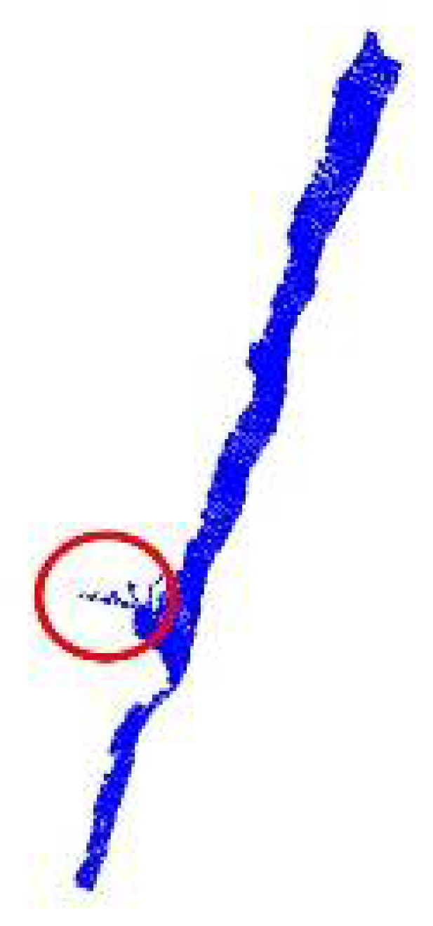
3.3.1. Extraction of Stem Point Cloud

Stem detection is a critical pre-processing step, which helps to accurately extract regions of interest (ROI) from noisy data. A faster RCNN model, a two-stage object detector, can be well applied to real-time detection for field stems. The model consists of three parts: the backbone, Region Proposal Network (RPN), and classification and regression module. The backbone is a convolutional layer used to extract the feature maps of input images. We adopted a residue network based on the ResNet50 as the backbone. At the same time, a feature pyramid network (FPN) was introduced into the backbone to improve the precision of the feature maps. RPN is a core network of the Faster RCNN, which is used to quickly generate potential regions of interest. The classification and regression module used the feature in each ROI to identify the ROI classes and generate the object bounding boxes.
Due to the limited number of labeled images, we adopted transfer learning technology to accelerate the convergence rate of model training in small sample datasets. The Faster RCNN model was initialized using weights pretrained from the Pascal VOC 2012 dataset, a large annotated image dataset open to the public. In the model training, we annotated a total of 1800 images with maize stems in the format of Pascal VOC 2012. These images included typical field scenes under different lighting intensities (e.g., strong lighting intensity, backlighting, and exposure) and field of views (e.g., close-distance and long-distance).
As the maize stem was the only object to be detected, the number of classes for the detection model was set to 2, i.e., background and stem. The Faster RCNN model training was performed using stochastic gradient descent (SGD) by the momentum optimizer with an initial learning rate of 0.005, a momentum of 0.9, and a weight decay of 0.0005. To improve the stability of model convergence, the learning rate was adjusted once every 5 epochs according to the ratio factor of 0.33. Based on the Pascal VOC 2012 training model, a total of 300 epochs were used to ensure the model convergence for the maize stem detection task. The model weights were saved for each iteration of the epoch. We chose the model weight with the highest accuracy for stem detection. Our dataset was trained on a graphic workstation, Dell Precision 7920 Tower (2 Xeon Silver 4214R @ 2.4 GHz CPU cores, 128 GB RAM, and NVIDIA GeForce RTX 3070 (8 GB)), using the operating system of Ubuntu 20.04 with Pytorch 1.6.0.
The stems detected by the Faster RCNN model were annotated with red bounding boxes based on their pixel coordinates. To better extract all of the pixel values of these stems based on the color information, the inner pixels of the bounding boxes were filled with red rectangles to highlight the stem pixels, named mask processing. Generally, the HSV color space represents the color characteristics of an object better than RGB space. Thus, we converted the RGB images with rectangular markers to the HSV space for post-processing. We defined the red mask threshold in the HSV space as follows:
L o w e r _ r e d = ( H u e min S a t u r a t i o n min V a l u e min ) U p p e r _ r e d = ( H u e max S a t u r a t i o n max V a l u e max )
where Huemin = 50, Saturationmin = 100, Valuemin = 100, Huemax = 70, Saturationmax = 255, and Valuemax = 255. According to the mask area, the pixel coordinates of stem regions could be extracted. To better distinguish the stem and background pixels in color image, the background pixels were replaced with zeros.
In general, the stem point cloud could be obtained based on RGB images and their corresponding depth images. All of the depth values of stems in the depth images could be extracted according to the coordinates of the stem pixels in the RGB images. These depth values were used to calculate the stem point cloud based on camera parameters. Specifically, stem point cloud extraction contains three steps: (1) judging whether each pixel coordinate belongs to the stem region according to the color information. It can be seen from the above that the color values of the stem area were not zeros, while the color values of the background pixels were zeros; (2) obtaining the non-zero coordinates of the RGB images, which were the stem coordinates of the depth images. Therefore, the depth values of stems could be extracted according to non-zero coordinates; and (3) generating a 3D point cloud from the depth values of stems and camera parameters. The equations for calculating the 3D points are:
P z = d c a m e r a _ f a c t o r P x = ( u c a m e r a _ c x ) × p z c a m e r a _ f x P y = ( v c a m e r a _ c y ) × p z c a m e r a _ f y
where Pz, Px, and Py represent the spatial coordinates of the 3D point, d is the depth value of the current pixel, u and v represent the pixel coordinates of the depth image, camera_cx and camera_cy determine the aperture center of the camera, camera_fx and camera_fy represent the focal length of the camera on the X and Y axes, respectively, and camera_factor is the scale factor for the depth image.
Normally, the extraction of stem point clouds is fulfilled after calculating all of the 3D points in the detected rectangle markers. However, the stem detection model will recognize all maize stems within the camera’s field of view, resulting in multiple maize stem point clouds for each frame. Additionally, one stem may be divided into multiple point clouds due to the occlusion of leaves. Figure 5a shows both cases. Thus, we need to accurately detect every stem and cluster point clouds belonging to the same stem. DBSCAN (Density-Based Spatial Clustering of Application with Noise) is an excellent clustering algorithm for point clouds that have significant density characteristics [44]. This algorithm can be used to cluster stem point clouds, since the point clouds belonging to the same stem have higher density characteristics. For DBSCAN, we set the threshold of neighborhood distance to 0.01 m, and the minimum number of points in the core point field to 20. To improve the efficiency of clustering, we introduced a KD-Tree search algorithm to search neighborhood points for DBSCAN.
In fact, the existing DBSCAN algorithm may have led to the mis-clustering of stem point clouds. For example, two plants were divided into four parts, which were considered to be four plants by DBSCAN, as shown in Figure 5a. As a result, we propose an improved DBSCAN, named with 2D-DBSCAN, as shown in Figure 5. 2D-DBSCAN can realize accurate clustering of stem point clouds. We assumed that the growth direction of crops is roughly parallel to the vertical axis (Y-axis) of the 3D coordinates. Then, a stem could be divided into several segments at different heights along the Y-axis. 2D-DBSCAN consists of three steps:
(i).
The stem point clouds in Figure 5a are projected onto the X-Z plane;
(ii).
DBSCAN is used to cluster each stem in a 2D plane, as shown in Figure 5b;
(iii).
The stem point clouds after clustering are restored to a 3D space, as shown in Figure 5c.
The white rectangle in Figure 5c indicates that the stems divided into multiple point clouds are clustered into one cluster. Note that the grey point cloud in Figure 5c is the missing part caused by occlusion or observation error. We give an in-depth introduction for the approach of filling the missing stem parts in the subsequent section.

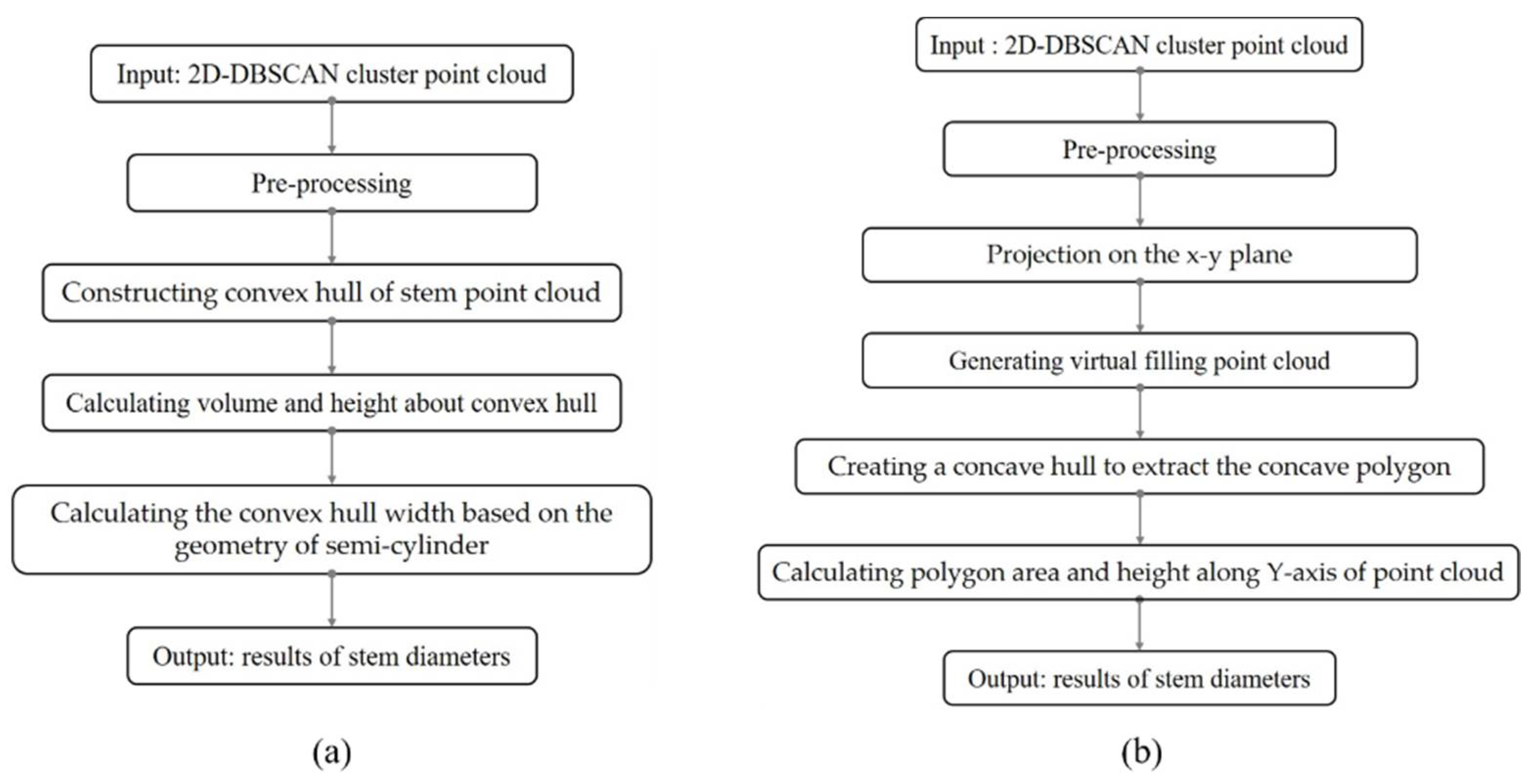
3.3.2. Estimation of Stem Diameters

We used two approaches, SD-PCCH and SD-PPC, to estimate the stem diameters of maize plants based on the point cloud clustering results. Among them, SD-PCCH used the volume and height of the point cloud convex hull to calculate the stem diameters. This approach assumed that the geometry of the detected maize stem parts was semi-cylindrical. The estimation process is shown in Figure 6a. SD-PPC is another approach to calculating the stem diameters, which is based on the projection of the point cloud on a 2D plane. Figure 6b shows the calculation process for SD-PPC.
SD-PCCH estimates the stem diameters by constructing a convex hull. The convex hull is a convex polygon formed by connecting the outermost points of a point cloud cluster. Convex hull detection is often used in object recognition, gesture recognition, and boundary detection. Thus, based on the geometry of the stem point cloud, the volume and height of the point cloud can be estimated by convex hull detection algorithms. SD-PCCH consists of four steps: (1) conducting pre-processing, such as statistical filtering, to remove the noise points from the point cloud cluster; (2) generating the point cloud convex hull based on the Convex Hull function in PCL, and obtaining the volume of the convex hull; (3) obtaining the minimum and maximum values of the Y-axis (Ymax and Ymin) for each stem point cloud; and (4) regarding the convex hull as a semi-cylinder based on the geometric characteristics of the stem. Note that the volume of the convex hull is half of the volume of the cylinder, because the point cloud covers only half of the stem. In step (iii), the height of the stem is calculated by:
H = Y max Y min
In this way, the stem diameters can be calculated as:
D = 2 2 V π H
where D and V are the width and volume of the semi-cylinder, respectively.
The estimation of stem diameters is effective using the convex hull of point clouds because the shape of the convex hull can be regarded as a semi-cylinder, which is similar to the real morphological structure of stems. However, this approach has a high requirement for the reconstruction precision of the stem point cloud. We know that the convex hull is composed of the vertex coordinates of the point cloud in all directions. Thus, even a small number of outliers will have a great influence on the measurement accuracy of stems. As shown in Figure 7, this image is a stem point cloud generated by 2D-DBSCAN clustering. We can see that there are a few outliers around the stem, such as the points within the red circular area. As a result, the convex hull generated by the point cloud has a larger volume than the actual stem, which will result in a larger stem diameter.
Here, we propose the second approach for measuring stem diameters, SD-PPC. As mentioned above, the depth values of the point cloud, that is, in the Z-axis direction, are sometimes inaccurate, which will affect the stem measurement accuracy, as shown in Figure 8a. However, mapping on the X–Y plane can eliminate the influence of inaccurate depth values, as shown in Figure 8b, which can accurately describe the characteristics of the stem. As a result, we used the projection of the stem point cloud on the X–Y plane to estimate the stem diameters, as shown in Figure 8. This approach consisted of seven steps. (1) Pre-processing. This step is the same as the pre-processing for SD-PCCH. (2) Establishing a plane projection model, which reassigns the Z values of the point cloud to zeros. In this way, the point cloud changes from 3D to 2D, as shown in Figure 8b. (3) Generating a virtual point cloud. This point cloud is used to fill in the missing data area due to leaf occlusion. The detailed method is described in Section 3.3.3. (4) Creating a concave hull representation of the projected point cloud to extract the concave polygon of the 2D point cloud. (5) Using the polygon area calculation function of PCL to obtain the area of the point cloud on the X–Y projection plane. (6) Searching the minimum and maximum values on the Y-axis according to the 2D point cloud coordinates. (7) Calculating the stem diameters with the following equation:
W s t e m = S a r e a Y max Y min
Here, Wstem is the stem diameter, Sarea is the polygon area of the point cloud on the X-Y projection plane, and the Ymax and Ymin represent the maximum and minimum values on the X-axis for 2D point cloud coordinates, respectively.

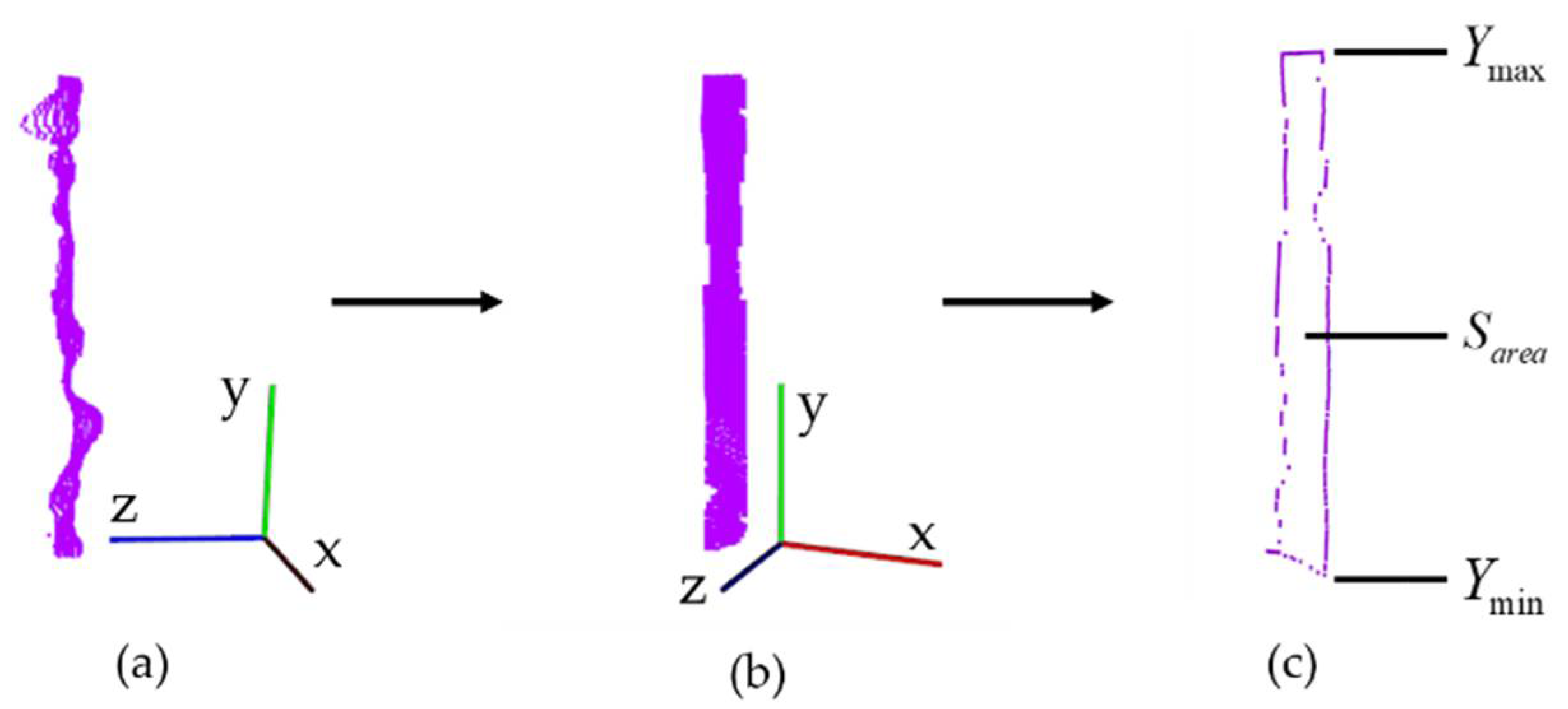
3.3.3. Filling Strategy for Missing Stem Parts in the Point Cloud

In the above section, we have realized the real-time estimation of stem diameters with our pipeline. However, the stem point cloud extracted usually has missing regions due to occlusions of plant leaves and holes in depth images of RGB-D cameras. These regions split the point cloud belonging to the same stem into two or more parts, which then affects the stem measurement results. In Section 3.3.1, we proposed the 2D-DBSCAN to accurate cluster the 3D stem points. In this section, we need to fill in the missing parts after clustering, as the gray point cloud shows in Figure 5c. Here, we propose a missing point cloud filling strategy based on the grid division, as shown in Figure 9, which consists of six steps:
(i).
Traversing the point cloud from the minimum value to the maximum value for the Y coordinate at a grid threshold interval of 0.003 m on the Y-axis. The range of the traversal is given by:
0 i < y max y min α ( i N + )
where i is the number of rows traversed on the Y-axis, α is 0.003 and indicates that the grid threshold of the traversal interval is 0.003 m, and ymax and ymin present the maximum value and minimum value of the point cloud coordinates on the Y-axis, respectively.
(ii).
For the region between row i and row i + 1 on the Y-axis during the traversal process, if the region has 3D points, that is, Equation (7) is satisfied, the region does not need to be filled;
y min + α · i < P y < y min + α · ( i + 1 )
where Py represents the coordinate value of existing 3D points along the Y-axis.
(iii).
If the requirements of the previous step are not met, point cloud filling is performed on the correspondence region;
(iv).
The number of points that need to be filled in this region can be expressed as:
K = x max x min α + 1 K N +
where xmax and xmin represent the maximum and minimum values of the point cloud on the X-axis, respectively, and K is the number of points that need to be filled.
(v).
The X and Y coordinates of the added points are given by:
{ X = x min + α · K j 0 < K j < K Y = y min + α · i
(vi).
The Z values of the points are set to 0 s. The reason is that the approach of calculating the stem diameters by SD-PPC does not need the Z values. Meanwhile, for the SD-PCCH approach, the convex hull already encloses the missing point cloud area, so there is also no need to calculate the Z values.
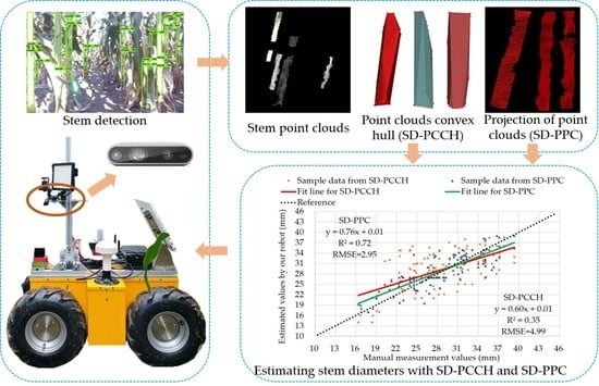
It is worth noting that SD-PCCH does not need to fill the point cloud for missing areas, because the approach for measuring the stem diameters only relies on the point cloud convex hull. On the contrary, the point cloud filling strategy is applicable to SD-PPC, because SD-PPC needs to extract the contour of the point cloud to calculate the stem diameters. Missing areas easily cause the wrong point cloud contour.

4. Results

4.1. Extraction of Stem Point Clouds

The extraction of stem point clouds consists of two steps: stem detection and point cloud extraction. Figure 10 shows the stem detection result of Faster RCNN under natural scenarios. These scenarios include strong lighting/backlighting, close-distance/long-distance, etc. Here, we used the mean average precision (mAP) to evaluate the performance of the stem detection model. mAP is the area covered by the PR (Precision–Recall) curve. mAP is computed as:
{ P r e c i s i o n = T P T P + F P R e c a l l = T P T P + F N A P = P r e c i s i o n N C m A P = q = 1 Q A P ( q ) Q
where TP, FP, and TN are true positive, false positive, and true negative, respectively, NC is the object number of C class in all images, and Q is the number of the detected object. Since the maize stem is the only detection object in our model, Q = 1. Figure 11 shows the loss curve and PR curve after model convergence. We found that mAP of stems was 67%.
The stem point cloud extracted based on the stem detection results is shown in Figure 12. Figure 12b shows the mask processing results based on the stem bounding box. Figure 12c shows the ROI of the extracted stem coordinates. Figure 12d shows the stem point cloud obtained from the depth image based on the RGB-D camera parameters. Noting that the stem area coordinates in the color image are completely the same as those in the depth image for RGB-D camera frames, the stem depth values in the depth image can be extracted according to the stem pixel location in the color image.

4.2. Visualization of Convex Hull and 2D Projection of Point Cloud

Building convex hulls and plane projections of stem point clouds are key steps to implement SD-PCCH and SD-PPC. Figure 13 shows the results of constructing convex hulls and plane projections of stem point clouds. Figure 13b shows the point clouds of each stem obtained by 2D-DBSCAN clustering from Figure 13a. Figure 13c,d show the convex hulls and plane projections of each stem extracted, respectively.

4.3. Point Cloud Filling

Figure 14 shows the results of our proposed point cloud filling strategy. The red areas are the point clouds obtained from the depth images, and the gray areas are the filling points. Our approach can join point clouds belonging to the same stem. It is worth noting that point cloud filling does not significantly affect the measurement results of stem diameters, but can avoid multiple measurements for the same observed stem in the SD-PPC. The reason is that split stems without filling will generate two or more point cloud contours.

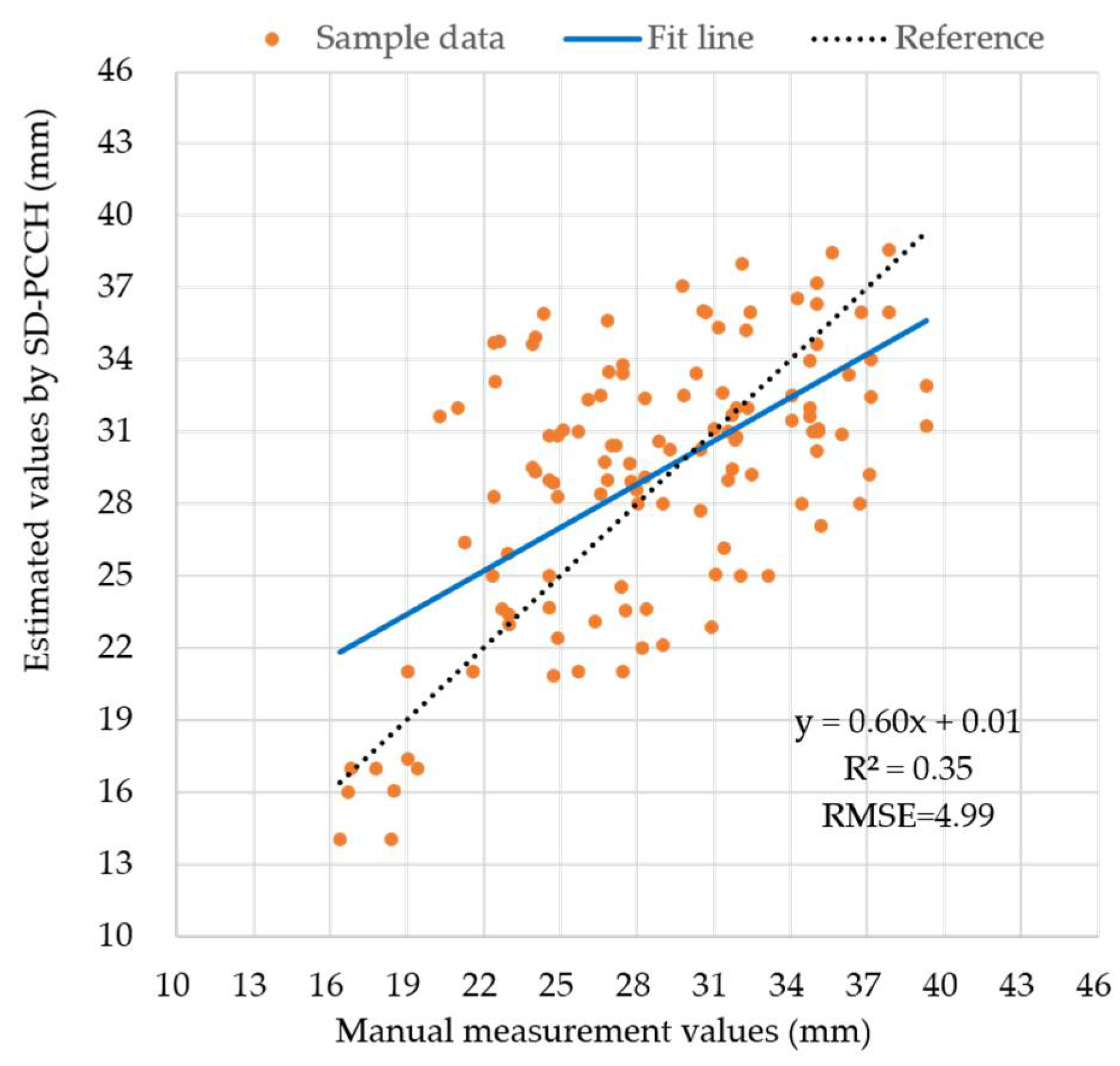
4.4. Stem Diameter Estimation with SD-PCCH and SD-PPC

In this section, we compare and analyze the stem diameter measurement results of our approaches with the manually measured values. Specifically, we evaluate the measurement accuracy of the two approaches, SD-PCCH and SD-PPC. Figure 15 and Figure 16 show the comparison results of our two approaches with the manual measurement values, where the horizontal and vertical coordinates represent the manual measurement values and the estimated values by our approaches, respectively. We used approximately 120 sets of stem samples from the testing dataset to estimate the stem diameters. We employed R2 and RMSE to evaluate the stem diameter estimation results. R2 shows the similarity between the estimated error and manual measurement error, where R2 = 1 means that the two types of error are the same. RMSE is the root-mean-square error, which emphasizes the deviations between the estimated values and manual measurement values. R2 and RMSE can be expressed as:
{ R 2 = 1 k = 1 n ( y k y k ) 2 k = 1 n ( y k y ¯ ) 2 R M S E = 1 n i = 1 n ( y k y k ) 2
where n is the data sample size, yk and y k are the k-th manual measurement value and estimated value, respectively, and y ¯ is the mean value of the manual measurement.
As can be seen from Figure 15 and Figure 16, the two approaches both achieved good results. The R2 and RMSE for SD-PCCH were 0.35 and 4.99 mm, respectively. The R2 and RMSE for SD-PPC were 0.72 and 2.95 mm, respectively. The experimental results showed that SD-PPC had better measurement accuracy than SD-PCCH. The reason is that the noise points of the depth values increased the volumes of the point cloud convex hulls, which caused the stem diameters to increase accordingly. On the contrary, the stem diameter estimation was not affected by the depth values of the point clouds for SD-PPC.
We also performed a statistical analysis of the measurement result distribution for the SD-PCCH, SD-PPC, and manual measurement values, as shown in Figure 17. The results showed that SD-PPC had a higher measurement accuracy than SD-PCCH, because the maximum, minimum, and median of SD-PPC were in better agreement with the results of the manual measurements than those of SD-PCCH. Meanwhile, according to the interquartile range, we found that the estimated values of SD-PPC were more concentrated around the median compared to those of SD-PCCH.
Additionally, we compared our stem diameter estimation results with those previously reported in [25,27]. We took R2, RMSE, and the Mean Absolute Error (MAE) as evaluation indexes. We add MAE as a comparison term because it is insensitive to outliers generated by the estimated values. This can better express the robustness of different algorithms to the stem diameter estimation results. MAE is computed as:
M A E = 1 n k = 1 n | y k y k |
where yk and y k are the k-th manual measurement value and estimated value, respectively. The comparison results are shown in Table 2. We found that our stem diameter estimation results were better than those of [25] and [27], because our R2 was greater and RMSE/MAE were smaller compared with those of [25] and [27]. Also, we compared SD-PCCH with SD-PPC, and found that SD-PPC had better estimation results than SD-PCCH in all metrics.

5. Discussion

Robotics-based high-throughput phenotyping has the potential to break the phenotypic bottleneck. Particularly, the study of HTP robots based on ground mobile platforms has been proven to be an effective way to accelerate automatic phenotyping [27,29,45]. Currently, HTP robots can realize non-contact measurement for crop morphological parameters by equipping them with sensing devices. In this study, we present a stem diameter measurement pipeline using a self-developed mobile phenotyping platform equipped with an RGB-D camera. The experiments show that the pipeline can meet the requirements of automatic measuring for maize stems in fields. More generally, our pipeline has good generalization capabilities for measuring the stem diameters of high crops in an ideal data collection condition. There is no denying that the existing measurement pipeline still has some challenges and limitations: (1). real-time performance. It is difficult for phenotyping robots to process large amounts of phenotype data online in field conditions due to the limitations of hardware devices; and (2). multi-parameter measurements. Our pipeline is currently used to estimate the stem diameters. How to achieve simultaneous measurement of multiple phenotypic parameters is a direction to be explored in the future. Currently, we need to address the following issues:
(i)
Improving the stem detection accuracy of convolutional neural network.
We used the existing two-stage object detector Faster-RCNN to identify field stems. The mAP of stem detection after network convergence was 67%. This may be caused by the strong lighting changes and the inconspicuous color characteristics of stems under the crop canopy. In the future, we hope to improve the detection accuracy of the detector by labeling more data sets and adjusting the network structure;
(ii)
Evaluating the 3D image quality of RealSense D435i.
RealSense D435i cameras have been proven to have excellent ranging performances under natural conditions. However, it is still necessary to evaluate the depth value accuracy for different crop organs to improve the 3D imaging quality. It will be helpful to improve the measurement accuracy of maize stem diameters;
(iii)
Improving the real-time phenotyping performances of our algorithm pipeline.
Currently, our algorithm pipeline is implemented on a graphics workstation. During our experiment, the bag recording function of ROS was used to obtain crop images in the field. These image data were parsed and used on the graphics workstation to run our phenotyping algorithm. In the future, our algorithm will be processed in real-time with an edge computing module on our HTP robot;
(iv)
Extending our algorithm pipeline to different crop varieties.
At present, maize crops are our main focus. However, the algorithm pipeline we proposed is expected to be applied to other common high-stem plants, such as sorghum, sugarcane, etc. Furthermore, we believe that our method can also be used for the measurement of the phenotypic parameters of various crop organs by only adjusting some necessary algorithm parameters.

6. Conclusions

This paper aimed to investigate a high-throughput phenotyping solution based on mobile robots and RGB-D sensing technologies. An in situ and inter-row stem diameter measurement pipeline for maize crops was proposed. In this pipeline, we used Faster RCNN to detect stems in color images and employed the point clouds converted from depth images to measure the maize stem diameters. We first solved the inaccurate clustering problem of stem point clouds caused by dense leave occlusions using a dimension reduction clustering algorithm based on DBSCAN. Then, we presented a point cloud filling strategy to fill the missing depth values of the stem point clouds. Finally, we proposed two stem diameter-estimation approaches (e.g., SD-PCCH and SD-PPC) by analyzing the geometric structures of the stem point clouds. Here, SD-PCCH and SD-PPC calculated the stem diameters using the 3D point cloud convex hull and the 2D projection of point clouds, respectively. The comparison of our approaches with other existing literatures showed that SD-PCCH and SD-PPC were effective in measuring stem diameters. In addition, since SD-PPC avoids the effect of depth noise on the estimation results, SD-PPC has higher measurement accuracy than SD-PCCH. By analyzing 120 test samples, the R2 and RMSE of SD-PPC were up to 0.72 and 2.95 mm, respectively.
Currently, greenhouse or controlled scenarios are still dominant for high-throughput phenotyping [9]. However, field-based crop cultivation is the main mode for food production. In-field phenotyping is still in the exploratory stage due to some intractable problems, such as intensive lighting changes, leaf-occlusion clutter, etc. The phenotyping robot we developed is exactly for in situ measuring the stem diameters of field crops. We hope that our algorithm pipeline can improve the phenotype screening efficiency, and can better serve breeders in the future. Meanwhile, we are also trying to integrate more advanced algorithms in our robot to realize online measurement for multiple phenotypic parameters, such as leaf length, leaf number, leaf angle, etc.

Author Contributions

Conceptualization, Z.F., Q.Q. and C.Z.; methodology, Z.F., Q.Q. and C.Z.; software, Z.F. and N.S.; validation, Z.F., Q.Q. and C.Z.; formal analysis, Q.Q.; investigation, Z.F., Q.Q. and C.Z.; resources, Q.Q., Q.F. and C.Z.; writing—original draft preparation, Z.F.; writing—review and editing, N.S., Q.Q., T.L., Q.F. and C.Z.; visualization, Z.F.; supervision, Q.Q. and C.Z.; project administration, Q.Q., Q.F. and C.Z.; funding acquisition, Q.Q., Q.F. and C.Z. All authors have read and agreed to the published version of the manuscript.

Funding

This research was funded by National Key Research and Development Program of China, grant number 2019YFE0125200, and National Natural Science Foundation of China, grant number 61973040.

Institutional Review Board Statement

Not applicable.

Informed Consent Statement

Not applicable.

Acknowledgments

The authors would like to thank Xuefeng Li and Qinghan Hu for many heuristic discussions, implementation assistance, and their kind encouragement.

Conflicts of Interest

The authors declare no conflict of interest.

References

  1. Chawade, A.; van Ham, J.; Blomquist, H.; Bagge, O.; Alexandersson, E.; Ortiz, R. High-Throughput Field-Phenotyping Tools for Plant Breeding and Precision Agriculture. Agronomy 2019, 9, 258. [Google Scholar] [CrossRef] [Green Version]
  2. Hunter, M.C.; Smith, R.G.; Schipanski, M.E.; Atwood, L.W.; Mortensen, D.A. Agriculture in 2050: Recalibrating Targets for Sustainable Intensification. BioScience 2017, 67, 386–391. [Google Scholar] [CrossRef] [Green Version]
  3. Hickey, L.T.; Hafeez, A.N.; Robinson, H.; Jackson, S.A.; Leal-Bertioli, S.C.M.; Tester, M.; Gao, C.; Godwin, I.D.; Hayes, B.J.; Wulff, B.B.H. Breeding crops to feed 10 billion. Nat. Biotechnol. 2019, 37, 744–754. [Google Scholar] [CrossRef] [PubMed] [Green Version]
  4. Li, D.; Quan, C.; Song, Z.; Li, X.; Yu, G.; Li, C.; Muhammad, A. High-Throughput Plant Phenotyping Platform (HT3P) as a Novel Tool for Estimating Agronomic Traits from the Lab to the Field. Front. Bioeng. Biotechnol. 2020, 8, 623705. [Google Scholar] [CrossRef]
  5. Mir, R.R.; Reynolds, M.; Pinto, F.; Khan, M.A.; Bhat, M.A. High-throughput phenotyping for crop improvement in the genomics era. Plant Sci. 2019, 282, 60–72. [Google Scholar] [CrossRef] [PubMed]
  6. Song, P.; Wang, J.; Guo, X.; Yang, W.; Zhao, C. High-throughput phenotyping: Breaking through the bottleneck in future crop breeding. Crop J. 2021, 9, 633–645. [Google Scholar] [CrossRef]
  7. Bailey-Serres, J.; Parker, J.E.; Ainsworth, E.A.; Oldroyd, G.E.D.; Schroeder, J.I. Genetic strategies for improving crop yields. Nature 2019, 575, 109–118. [Google Scholar] [CrossRef] [Green Version]
  8. Yang, G.; Liu, J.; Zhao, C.; Li, Z.; Huang, Y.; Yu, H.; Xu, B.; Yang, X.; Zhu, D.; Zhang, X.; et al. Unmanned Aerial Vehicle Remote Sensing for Field-Based Crop Phenotyping: Current Status and Perspectives. Front. Plant Sci. 2017, 8, 1111. [Google Scholar] [CrossRef]
  9. Atefi, A.; Ge, Y.; Pitla, S.; Schnable, J. Robotic Technologies for High-Throughput Plant Phenotyping: Contemporary Reviews and Future Perspectives. Front. Plant Sci. 2021, 12, 611940. [Google Scholar] [CrossRef]
  10. Robertson, D.J.; Julias, M.; Lee, S.Y.; Cook, D.D. Maize Stalk Lodging: Morphological Determinants of Stalk Strength. Crop Sci. 2017, 57, 926–934. [Google Scholar] [CrossRef] [Green Version]
  11. Vit, A.; Shani, G. Comparing RGB-D Sensors for Close Range Outdoor Agricultural Phenotyping. Sensors 2018, 18, 4413. [Google Scholar] [CrossRef] [Green Version]
  12. Fan, Z.; Sun, N.; Qiu, Q.; Li, T.; Zhao, C. Depth Ranging Performance Evaluation and Improvement for RGB-D Cameras on Field-Based High-Throughput Phenotyping Robots *. In Proceedings of the 2021 IEEE/RSJ International Conference on Intelligent Robots and Systems (IROS), Prague, Czech Republic, 27 September–1 October 2021; pp. 3299–3304. [Google Scholar]
  13. Araus, J.L.; Kefauver, S.C.; Diaz, O.V.; Gracia-Romero, A.; Rezzouk, F.Z.; Segarra, J.; Buchaillot, M.L.; Chang-Espino, M.; Vatter, T.; Sanchez-Bragado, R.; et al. Crop phenotyping in a context of Global Change: What to measure and how to do it. J. Integr. Plant Biol. 2021. [Google Scholar] [CrossRef] [PubMed]
  14. Jangra, S.; Chaudhary, V.; Yadav, R.C.; Yadav, N.R. High-Throughput Phenotyping: A Platform to Accelerate Crop Improvement. Phenomics 2021, 1, 31–53. [Google Scholar] [CrossRef]
  15. Virlet, N.; Sabermanesh, K.; Sadeghi-Tehran, P.; Hawkesford, M.J. Field Scanalyzer: An automated robotic field phenotyping platform for detailed crop monitoring. Funct. Plant Biol. 2017, 44, 143–153. [Google Scholar] [CrossRef] [PubMed] [Green Version]
  16. Yang, W.; Feng, H.; Zhang, X.; Zhang, J.; Doonan, J.H.; Batchelor, W.D.; Xiong, L.; Yan, J. Crop Phenomics and High-Throughput Phenotyping: Past Decades, Current Challenges, and Future Perspectives. Mol. Plant 2020, 13, 187–214. [Google Scholar] [CrossRef] [PubMed] [Green Version]
  17. Jang, G.; Kim, J.; Yu, J.-K.; Kim, H.-J.; Kim, Y.; Kim, D.-W.; Kim, K.-H.; Lee, C.W.; Chung, Y.S. Review: Cost-Effective Unmanned Aerial Vehicle (UAV) Platform for Field Plant Breeding Application. Remote Sens. 2020, 12, 998. [Google Scholar] [CrossRef] [Green Version]
  18. Araus, J.L.; Kefauver, S.C. Breeding to adapt agriculture to climate change: Affordable phenotyping solutions. Curr. Opin. Plant Biol. 2018, 45, 237–247. [Google Scholar] [CrossRef]
  19. Jin, X.; Zarco-Tejada, P.J.; Schmidhalter, U.; Reynolds, M.P.; Hawkesford, M.J.; Varshney, R.K.; Yang, T.; Nie, C.; Li, Z.; Ming, B.; et al. High-Throughput Estimation of Crop Traits: A Review of Ground and Aerial Phenotyping Platforms. IEEE Geosci. Remote Sens. Mag. 2021, 9, 200–231. [Google Scholar] [CrossRef]
  20. Shafiekhani, A.; Kadam, S.; Fritschi, F.B.; DeSouza, G.N. Vinobot and Vinoculer: Two Robotic Platforms for High-Throughput Field Phenotyping. Sensors 2017, 17, 214. [Google Scholar] [CrossRef]
  21. Shafiekhani, A.; Fritschi, F.B.; DeSouza, G.N. Vinobot and vinoculer: From real to simulated platforms. In Proceedings of the SPIE Commercial + Scientific Sensing and Imaging, Orlando, FL, USA, 15–19 April 2018. [Google Scholar]
  22. Ahmadi, A.; Nardi, L.; Chebrolu, N.; Stachniss, C. Visual Servoing-based Navigation for Monitoring Row-Crop Fields. In Proceedings of the 2020 IEEE International Conference on Robotics and Automation (ICRA), Paris, France, 31 May–31 August 2020; pp. 4920–4926. [Google Scholar]
  23. Mueller-Sim, T.; Jenkins, M.; Abel, J.; Kantor, G. The Robotanist: A ground-based agricultural robot for high-throughput crop phenotyping. In Proceedings of the 2017 IEEE International Conference on Robotics and Automation (ICRA), Singapore, 29 May–3 June 2017; pp. 3634–3639. [Google Scholar]
  24. Kayacan, E.; Young, S.N.; Peschel, J.M.; Chowdhary, G. High-precision control of tracked field robots in the presence of unknown traction coefficients. J. Field Robot. 2018, 35, 1050–1062. [Google Scholar] [CrossRef]
  25. Bao, Y.; Tang, L.; Srinivasan, S.; Schnable, P.S. Field-based architectural traits characterisation of maize plant using time-of-flight 3D imaging. Biosyst. Eng. 2019, 178, 86–101. [Google Scholar] [CrossRef]
  26. Baharav, T.; Bariya, M.; Zakhor, A. In Situ Height and Width Estimation of Sorghum Plants from 2.5 d Infrared Images. Electron. Imaging 2017, 2017, 122–135. [Google Scholar] [CrossRef] [Green Version]
  27. Baweja, H.S.; Parhar, T.; Mirbod, O.; Nuske, S. StalkNet: A Deep Learning Pipeline for High-Throughput Measurement of Plant Stalk Count and Stalk Width. In Field and Service Robotics; Springer Proceedings in Advanced Robotics; Springer: Berlin/Heidelberg, Germany, 2018; pp. 271–284. [Google Scholar]
  28. Parhar, T.; Baweja, H.; Jenkins, M.; Kantor, G. A Deep Learning-Based Stalk Grasping Pipeline. In Proceedings of the 2018 IEEE International Conference on Robotics and Automation (ICRA), Brisbane, Australia, 21–25 May 2018; pp. 6161–6167. [Google Scholar]
  29. Young, S.N.; Kayacan, E.; Peschel, J.M. Design and field evaluation of a ground robot for high-throughput phenotyping of energy sorghum. Precis. Agric. 2018, 20, 697–722. [Google Scholar] [CrossRef] [Green Version]
  30. Zhang, Z.; Kayacan, E.; Thompson, B.; Chowdhary, G. High precision control and deep learning-based corn stand counting algorithms for agricultural robot. Auton. Robot. 2020, 44, 1289–1302. [Google Scholar] [CrossRef]
  31. Qiu, Q.; Sun, N.; Bai, H.; Wang, N.; Fan, Z.; Wang, Y.; Meng, Z.; Li, B.; Cong, Y. Field-Based High-Throughput Phenotyping for Maize Plant Using 3D LiDAR Point Cloud Generated With a “Phenomobile”. Front. Plant Sci. 2019, 10, 554. [Google Scholar] [CrossRef] [PubMed] [Green Version]
  32. Qiu, Q.; Fan, Z.; Meng, Z.; Zhang, Q.; Cong, Y.; Li, B.; Wang, N.; Zhao, C. Extended Ackerman Steering Principle for the coordinated movement control of a four wheel drive agricultural mobile robot. Comput. Electron. Agric. 2018, 152, 40–50. [Google Scholar] [CrossRef]
  33. Qiu, R.; Wei, S.; Zhang, M.; Li, H.; Sun, H.; Liu, G.; Li, M. Sensors for measuring plant phenotyping: A review. Int. J. Agric. Biol. Eng. 2018, 11, 1–17. [Google Scholar] [CrossRef] [Green Version]
  34. Jin, S.; Su, Y.; Gao, S.; Wu, F.; Ma, Q.; Xu, K.; Ma, Q.; Hu, T.; Liu, J.; Pang, S.; et al. Separating the Structural Components of Maize for Field Phenotyping Using Terrestrial LiDAR Data and Deep Convolutional Neural Networks. IEEE Trans. Geosci. Remote Sens. 2020, 58, 2644–2658. [Google Scholar] [CrossRef]
  35. Kazmi, W.; Foix, S.; Alenyà, G.; Andersen, H.J. Indoor and outdoor depth imaging of leaves with time-of-flight and stereo vision sensors: Analysis and comparison. ISPRS J. Photogramm. Remote Sens. 2014, 88, 128–146. [Google Scholar] [CrossRef] [Green Version]
  36. Hämmerle, M.; Höfle, B. Mobile low-cost 3D camera maize crop height measurements under field conditions. Precis. Agric. 2017, 19, 630–647. [Google Scholar] [CrossRef]
  37. Kurtser, P.; Ringdahl, O.; Rotstein, N.; Berenstein, R.; Edan, Y. In-Field Grape Cluster Size Assessment for Vine Yield Estimation Using a Mobile Robot and a Consumer Level RGB-D Camera. IEEE Robot. Autom. Lett. 2020, 5, 2031–2038. [Google Scholar] [CrossRef]
  38. Atefi, A.; Ge, Y.; Pitla, S.; Schnable, J. Robotic Detection and Grasp of Maize and Sorghum: Stem Measurement with Contact. Robotics 2020, 9, 58. [Google Scholar] [CrossRef]
  39. Li, Y.; Wen, W.; Guo, X.; Yu, Z.; Gu, S.; Yan, H.; Zhao, C. High-throughput phenotyping analysis of maize at the seedling stage using end-to-end segmentation network. PLoS ONE 2021, 16, e0241528. [Google Scholar] [CrossRef] [PubMed]
  40. Liu, F.; Hu, P.; Zheng, B.; Duan, T.; Zhu, B.; Guo, Y. A field-based high-throughput method for acquiring canopy architecture using unmanned aerial vehicle images. Agric. For. Meteorol. 2021, 296, 108231. [Google Scholar] [CrossRef]
  41. Zermas, D.; Morellas, V.; Mulla, D.; Papanikolopoulos, N. 3D model processing for high throughput phenotype extraction–the case of corn. Comput. Electron. Agric. 2020, 172, 105047. [Google Scholar] [CrossRef]
  42. Erndwein, L.; Cook, D.D.; Robertson, D.J.; Sparks, E.E. Field-based mechanical phenotyping of cereal crops to assess lodging resistance. Appl. Plant Sci. 2020, 8, e11382. [Google Scholar] [CrossRef]
  43. Fan, Z.; Sun, N.; Qiu, Q.; Li, T.; Zhao, C. A High-Throughput Phenotyping Robot for Measuring Stalk Diameters of Maize Crops. In Proceedings of the 2021 IEEE 11th Annual International Conference on CYBER Technology in Automation, Control, and Intelligent Systems (CYBER), Jiaxing, China, 27–31 July 2021; pp. 128–133. [Google Scholar]
  44. Mahesh Kumar, K.; Rama Mohan Reddy, A. A fast DBSCAN clustering algorithm by accelerating neighbor searching using Groups method. Pattern Recognit. 2016, 58, 39–48. [Google Scholar] [CrossRef]
  45. Vázquez-Arellano, M.; Reiser, D.; Paraforos, D.S.; Garrido-Izard, M.; Burce, M.E.C.; Griepentrog, H.W. 3-D reconstruction of maize plants using a time-of-flight camera. Comput. Electron. Agric. 2018, 145, 235–247. [Google Scholar] [CrossRef]
Figure 1. The schematic of HTP robot platform. (a) is the system control schematic. (b) (1) mast; (2) display screen; (3) power and communication interfaces; (4) sensor trays; (5) IPC; (6) GPS receiver; (7) laser scanner; (8) robot body.
Remotesensing 14 01030 g001
Figure 2. The experimental scheme.
Remotesensing 14 01030 g002
Figure 3. The experimental scenarios. (a) crop rows; (b) aisle.
Remotesensing 14 01030 g003
Figure 4. The comprehensive framework for calculating the stem diameters.
Remotesensing 14 01030 g004
Figure 5. Point cloud clustering strategy based on improved DBSCAN. (a) 3D stem point clouds; (b) projections of point clouds on the x-z plane; (c) stems that split into multiple point clouds clustered into one cluster.
Remotesensing 14 01030 g005
Figure 6. Two approaches for estimating the stem diameters. (a) SD-PCCH; (b) SD-PPC.
Remotesensing 14 01030 g006
Figure 7. The point cloud with outliers.
Remotesensing 14 01030 g007
Figure 8. 2D point cloud contour extraction. (a) 3D point cloud. (b) the projection of the cloud on the X-Y plane. (c) the point cloud contour used to generate concave hull.
Remotesensing 14 01030 g008
Figure 9. The point cloud filling strategy.
Remotesensing 14 01030 g009
Figure 10. The stem detection by Faster RCNN under natural scenarios. (a) long-distance and strong lighting intensity; (b) close-distance and backlighting; (c) close-distance; (d) backlighting; (e) strong lighting intensity; (f) long-distance.
Remotesensing 14 01030 g010
Figure 11. The loss curve and PR curve after model convergence.
Remotesensing 14 01030 g011
Figure 12. The stem point cloud extraction based on target bounding box. (a) Stem bounding box; (b) mask processing; (c) ROI of stem pixels; (d) stem point clouds.
Remotesensing 14 01030 g012
Figure 13. Convex hulls and plane projections of stem point clouds. (a) Stem point clouds; (b) point clouds clustered based on 2D-DBSCAN; (c) convex hulls; (d) plane projections of point clouds.
Remotesensing 14 01030 g013
Figure 14. The point cloud filling results.
Remotesensing 14 01030 g014
Figure 15. The comparison results of the stem diameter estimation based on SD-PCCH and the manual measurement values.
Remotesensing 14 01030 g015
Figure 16. The comparison results of the stem diameter estimation based on SD-PPC and the manual measurement values.
Remotesensing 14 01030 g016
Figure 17. The measurement result distribution of the stem diameters by SD-PCCH, SD-PPC, and manual measurement.
Remotesensing 14 01030 g017
Table 1. The specifications and parameters of our HTP robot.
SpecificationsParametersSpecificationsParameters
Size0.80 m × 0.45 m × 0.40 mMass40 kg
Operating temperature−15–50 °CCarrying capacity30 kg
Working time4 hVoltage24 V
Climbing gradient25°Maximum velocity0.30 m/s
Mobile modeWheeled modelObstacle clearing capability0.15 m
Steering modeDifferential steeringGround clearance0.10 m
Working environmentIn-rowApplied coding interfaceROS, C++, Python
Table 2. The comprehensive evaluation results for SD-PCCH and SD-PPC.
Stem Diameter EstimationOur Algorithms[27][25]
SD-PCCHSD-PPC
R20.350.72-0.27
RMSE (mm)4.992.95-5.29
MAE (mm)3.982.363.874.43
Publisher’s Note: MDPI stays neutral with regard to jurisdictional claims in published maps and institutional affiliations.

