
A Cloud-Based Mapping Approach Using Deep Learning and Very-High Spatial Resolution Earth Observation Data to Facilitate the SDG 11.7.1 Indicator Computation


Abstract
:1. Introduction
2. Materials and Methods
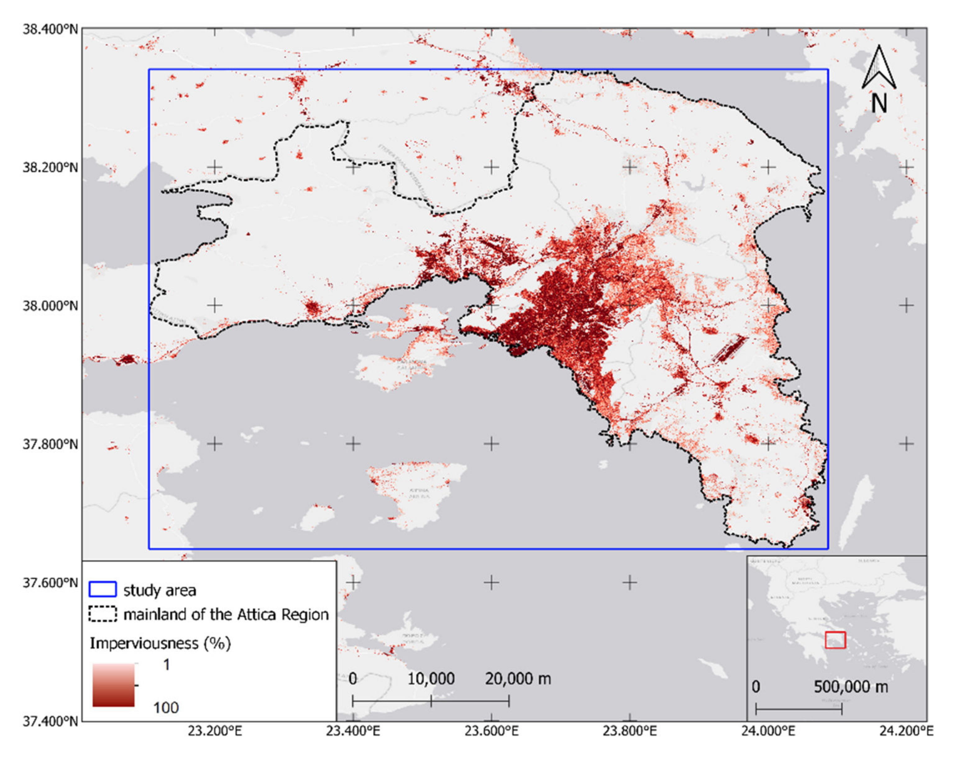
2.1. Study Area
2.2. Overall Workflow
2.3. Satellite Data
2.4. Ancillary Data and Preprocessing
2.5. Processing
2.5.1. Built-Up Area and Urban Extent
2.5.2. Urban Open Space
2.5.3. Land Allocated to Streets
2.5.4. Accuracy Assessment and Indicator Calculation
3. Results
3.1. Accuracy Metrics
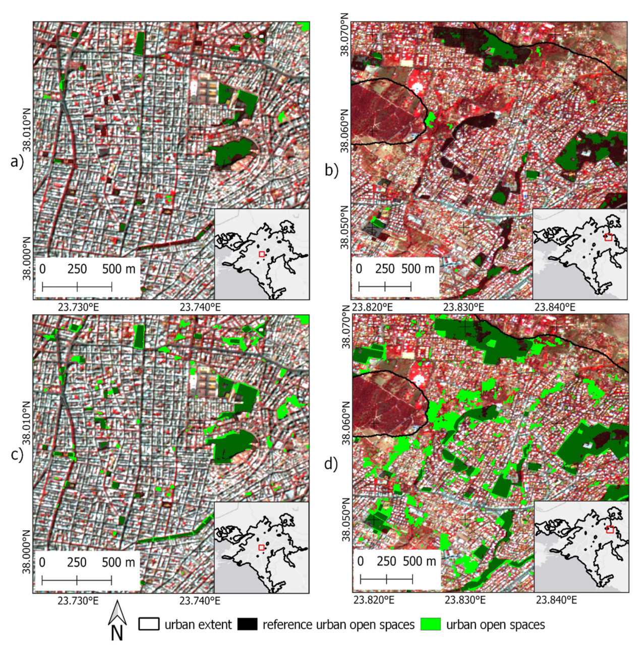
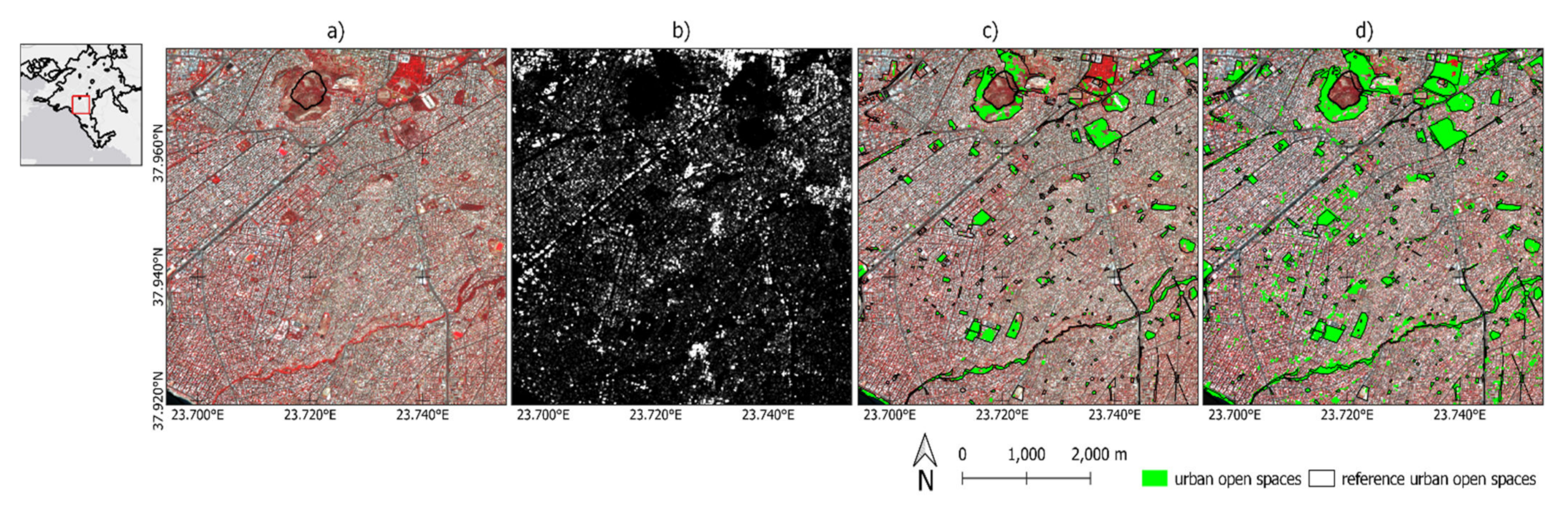
3.2. Visual Assessment of Results
4. Discussion
5. Conclusions
Author Contributions
Funding
Acknowledgments
Conflicts of Interest
References
- Pesaresi, M.; Melchiorri, M.; Siragusa, A.; Kemper, T. Atlas of the Human Planet 2016; Mapping Humam Presence on Earth with the Global Human Settlement Layer; Publications Office of the European Union: Luxembourg, 2016; ISBN 9789279620225. [Google Scholar]
- International Expert Panel on Science and the Future of Cities. Science and the Future of Cities; International Expert Panel on Science and the Future of Cities: London, UK; Melbourne, Australia, 2018. [Google Scholar]
- United Nations. World Population Prospects 2019: Highlights; United Nations: New York, NY, USA, 2019; pp. 1–39. [Google Scholar]
- Wai, A.T.P.; Nitivattananon, V.; Kim, S.M. Multi-stakeholder and multi-benefit approaches for enhanced utilization of public open spaces in Mandalay city, Myanmar. Sustain. Cities Soc. 2018, 37, 323–335. [Google Scholar] [CrossRef]
- García-Gómez, H.; Aguillaume, L.; Izquieta-Rojano, S.; Valiño, F.; Àvila, A.; Elustondo, D.; Santamaría, J.M.; Alastuey, A.; Calvete-Sogo, H.; González-Fernández, I.; et al. Atmospheric pollutants in peri-urban forests of Quercus ilex: Evidence of pollution abatement and threats for vegetation. Environ. Sci. Pollut. Res. 2016, 23, 6400–6413. [Google Scholar] [CrossRef] [PubMed] [Green Version]
- Baró, F.; Chaparro, L.; Gómez-Baggethun, E.; Langemeyer, J.; Nowak, D.J.; Terradas, J. Contribution of Ecosystem Services to Air Quality and Climate Change Mitigation Policies: The Case of Urban Forests in Barcelona, Spain. Ambio 2014, 43, 466–479. [Google Scholar] [CrossRef] [PubMed] [Green Version]
- Hamada, S.; Ohta, T. Seasonal variations in the cooling effect of urban green areas on surrounding urban areas. Urban For. Urban Green. 2010, 9, 15–24. [Google Scholar] [CrossRef]
- Moreira, T.C.L.; Polize, J.L.; Brito, M.; da Silva Filho, D.F.; Chiavegato Filho, A.D.P.; Viana, M.C.; Andrade, L.H.; Mauad, T. Assessing the impact of urban environment and green infrastructure on mental health: Results from the São Paulo Megacity Mental Health Survey. J. Expo. Sci. Environ. Epidemiol. 2021, 1–8. [Google Scholar] [CrossRef]
- Ahirrao, P.; Khan, S. Assessing Public Open Spaces: A Case of City Nagpur, India. Sustainbility 2021, 13, 4997. [Google Scholar] [CrossRef]
- United States Indicator 11.7.1. Average Share of the Built-Up Area of Cities That Is Open Space for Public Use for All, by Sex, Age and Persons with Disabilities; Eurostat: Luxembourg, 2018. [Google Scholar]
- Aguilar, R.; Kuffer, M. Cloud Computation Using High-Resolution Images for Improving the SDG Indicator on Open Spaces. Remote Sens. 2020, 12, 1144. [Google Scholar] [CrossRef] [Green Version]
- Giuliani, G.; Petri, E.; Interwies, E.; Vysna, V.; Guigoz, Y.; Ray, N.; Dickie, I. Modelling Accessibility to Urban Green Areas Using Open Earth Observations Data: A Novel Approach to Support the Urban SDG in Four European Cities. Remote Sens. 2021, 13, 422. [Google Scholar] [CrossRef]
- Ludwig, C.; Hecht, R.; Lautenbach, S.; Schorcht, M.; Zipf, A. Mapping Public Urban Green Spaces Based on OpenStreetMap and Sentinel-2 Imagery Using Belief Functions. ISPRS Int. J. Geo-Inf. 2021, 10, 251. [Google Scholar] [CrossRef]
- Prakash, M.; Ramage, S.; Kavvada, A.; Goodman, S. Open Earth Observations for Sustainable Urban Development. Remote Sens. 2020, 12, 1646. [Google Scholar] [CrossRef]
- Alamanos, A.; Linnane, S. Estimating SDG Indicators in Data-Scarce Areas: The Transition to the Use of New Technologies and Multidisciplinary Studies. Earth 2021, 2, 37. [Google Scholar] [CrossRef]
- Ferreira, B.; Iten, M.; Silva, R.G. Monitoring sustainable development by means of earth observation data and machine learning: A review. Environ. Sci. Eur. 2020, 32, 120. [Google Scholar] [CrossRef]
- Kearney, S.P.; Coops, N.C.; Sethi, S.; Stenhouse, G.B. Maintaining accurate, current, rural road network data: An extraction and updating routine using RapidEye, participatory GIS and deep learning. Int. J. Appl. Earth Obs. Geoinf. 2020, 87, 102031. [Google Scholar] [CrossRef]
- Zhang, C.; Sargent, I.; Pan, X.; Li, H.; Gardiner, A.; Hare, J.; Atkinson, P.M. An object-based convolutional neural network (OCNN) for urban land use classification. Remote Sens. Environ. 2018, 216, 57–70. [Google Scholar] [CrossRef] [Green Version]
- Chen, B.; Tu, Y.; Song, Y.; Theobald, D.M.; Zhang, T.; Ren, Z.; Li, X.; Yang, J.; Wang, J.; Wang, X.; et al. Mapping essential urban land use categories with open big data: Results for five metropolitan areas in the United States of America. ISPRS J. Photogramm. Remote Sens. 2021, 178, 203–218. [Google Scholar] [CrossRef]
- Habitat. The Street Connectivity Index (SCI) of Six Municipalities in Jalisco State, Mexico; United Nations: New York, NY, USA, 2016; pp. 1–66. [Google Scholar]
- Pesaresi, M.; Huadong, G.; Blaes, X.; Ehrlich, D.; Ferri, S.; Gueguen, L.; Halkia, M.; Kauffmann, M.; Kemper, T.; Lu, L.; et al. A global human settlement layer from optical HR/VHR RS data: Concept and first results. IEEE J. Sel. Top. Appl. Earth Obs. Remote Sens. 2013, 6, 2102–2131. [Google Scholar] [CrossRef]
- Ehrlich, D.; Kemper, T.; Pesaresi, M.; Corbane, C. Built-up area and population density: Two Essential Societal Variables to address climate hazard impact. Environ. Sci. Policy 2018, 90, 73–82. [Google Scholar] [CrossRef]
- Houborg, R.; McCabe, M.F. A Cubesat enabled Spatio-Temporal Enhancement Method (CESTEM) utilizing Planet, Landsat and MODIS data. Remote Sens. Environ. 2018, 209, 211–226. [Google Scholar] [CrossRef]
- Planet Team. Planet Application Program Interface. In Space for Life on Earth; Planet Publications: Fort Mill, SC, USA, 2017; Available online: https://www.planet.com/pulse/publications/ (accessed on 21 January 2022).
- Yin, J.; Dong, J.; Hamm, N.A.S.; Li, Z.; Wang, J.; Xing, H.; Fu, P. Integrating remote sensing and geospatial big data for urban land use mapping: A review. Int. J. Appl. Earth Obs. Geoinf. 2021, 103, 102514. [Google Scholar] [CrossRef]
- Jozdani, S.E.; Johnson, B.A.; Chen, D. Comparing Deep Neural Networks, Ensemble Classifiers, and Support Vector Machine Algorithms for Object-Based Urban Land Use/Land Cover Classification. Remote Sens. 2019, 11, 1713. [Google Scholar] [CrossRef] [Green Version]
- UN-Habitat. SDG Indicator 11.7.1 Training Module: Public Space; UN-Habitat: Nairobi, Kenya, 2018. [Google Scholar]
- Chen, Y.; Weng, Q.; Tang, L.; Liu, Q.; Zhang, X.; Bilal, M. Automatic mapping of urban green spaces using a geospatial neural network. GISci. Remote Sens. 2021, 58, 624–642. [Google Scholar] [CrossRef]
- Huang, B.; Zhao, B.; Song, Y. Urban land-use mapping using a deep convolutional neural network with high spatial resolution multispectral remote sensing imagery. Remote Sens. Environ. 2018, 214, 73–86. [Google Scholar] [CrossRef]
- Yao, Y.; Yan, X.; Luo, P.; Liang, Y.; Ren, S.; Hu, Y.; Han, J.; Guan, Q. Classifying land-use patterns by integrating time-series electricity data and high-spatial resolution remote sensing imagery. Int. J. Appl. Earth Obs. Geoinf. 2022, 106, 102664. [Google Scholar] [CrossRef]
- Tu, Y.; Chen, B.; Lang, W.; Chen, T.; Li, M.; Zhang, T.; Xu, B. Uncovering the Nature of Urban Land Use Composition Using Multi-Source Open Big Data with Ensemble Learning. Remote Sens. 2021, 13, 4241. [Google Scholar] [CrossRef]
- Hou, Y.; Liu, Z.; Zhang, T.; Li, Y. C-UNet: Complement UNet for Remote Sensing Road Extraction. Sensors 2021, 21, 2153. [Google Scholar] [CrossRef]
- Xu, Z.; Zhou, Y.; Wang, S.; Wang, L.; Li, F.; Wang, S.; Wang, Z. A Novel Intelligent Classification Method for Urban Green Space Based on High-Resolution Remote Sensing Images. Remote Sens. 2020, 12, 3845. [Google Scholar] [CrossRef]
- Zhang, Z.; Liu, Q.; Wang, Y. Road Extraction by Deep Residual U-Net. IEEE Geosci. Remote Sens. Lett. 2018, 15, 749–753. [Google Scholar] [CrossRef] [Green Version]
- Ma, Y.; Wu, H.; Wang, L.; Huang, B.; Ranjan, R.; Zomaya, A.; Jie, W. Remote sensing big data computing: Challenges and opportunities. Futur. Gener. Comput. Syst. 2015, 51, 47–60. [Google Scholar] [CrossRef] [Green Version]
- Huerta, R.E.; Yépez, F.D.; Lozano-García, D.F.; Guerra Cobián, V.H.; Ferriño Fierro, A.L.; de León Gómez, H.; Cavazos González, R.A.; Vargas-Martínez, A. Mapping Urban Green Spaces at the Metropolitan Level Using Very High Resolution Satellite Imagery and Deep Learning Techniques for Semantic Segmentation. Remote Sens. 2021, 13, 2031. [Google Scholar] [CrossRef]
- UN-Habitat. National Sample of Cities—A Model Approach to Monitoring and Reporting Performance of Cities at National Levels. 2017. Available online: https://unhabitat.org/national-sample-of-cities (accessed on 21 October 2020).
- Fameli, K.M.; Assimakopoulos, V.D. Development of a road transport emission inventory for Greece and the Greater Athens Area: Effects of important parameters. Sci. Total Environ. 2015, 505, 770–786. [Google Scholar] [CrossRef] [Green Version]
- Georgakis, C.; Santamouris, M. Determination of the Surface and Canopy Urban Heat Island in Athens Central Zone Using Advanced Monitoring. Climate 2017, 5, 97. [Google Scholar] [CrossRef] [Green Version]
- Salvati, L. Neither ordinary nor global: A reflection on the ‘extra-ordinary’ expansion of Athens. Urban Plan. Transp. Res. 2014, 2, 49–56. [Google Scholar] [CrossRef]
- Google Colaboratory. Frequently Asked Questions. Available online: https://research.google.com/colaboratory/faq.html (accessed on 17 January 2022).
- Gorelick, N.; Hancher, M.; Dixon, M.; Ilyushchenko, S.; Thau, D.; Moore, R. Google Earth Engine: Planetary-scale geospatial analysis for everyone. Remote Sens. Environ. 2017, 202, 18–27. [Google Scholar] [CrossRef]
- Abadi, M.; Agarwal, A.; Barham, P.; Brevdo, E.; Chen, Z.; Citro, C.; Corrado, G.S.; Davis, A.; Dean, J.; Devin, M.; et al. TensorFlow: Large-Scale Machine Learning on Heterogeneous Distributed Systems. arXiv 2015, arXiv:1603.04467. [Google Scholar]
- Chollet, F. Keras. Available online: https://github.com/fchollet/keras (accessed on 1 November 2021).
- Huang, H.; Roy, D.P. Characterization of Planetscope-0 Planetscope-1 surface reflectance and normalized difference vegetation index continuity. Sci. Remote Sens. 2021, 3, 100014. [Google Scholar] [CrossRef]
- Kotchenova, S.Y.; Vermote, E.F.; Matarrese, R.; Klemm, F.J., Jr. Validation of a vector version of the 6S radiative transfer code for atmospheric correction of satellite data Part I: Path radiance. Appl. Opt. 2006, 45, 6762. [Google Scholar] [CrossRef] [Green Version]
- D’Andrimont, R.; Lemoine, G.; van der Velde, M. Targeted Grassland Monitoring at Parcel Level Using Sentinels, Street-Level Images and Field Observations. Remote Sens. 2018, 10, 1300. [Google Scholar] [CrossRef] [Green Version]
- Copernicus Imperviousness. Available online: https://land.copernicus.eu/pan-european/high-resolution-layers/imperviousness (accessed on 17 January 2022).
- OpenStreetMap. Available online: https://www.openstreetmap.org/ (accessed on 17 January 2022).
- Schultz, M.; Voss, J.; Auer, M.; Carter, S.; Zipf, A. Open land cover from OpenStreetMap and remote sensing. Int. J. Appl. Earth Obs. Geoinf. 2017, 63, 206–213. [Google Scholar] [CrossRef]
- Vargas-Munoz, J.E.; Srivastava, S.; Tuia, D.; Falcao, A.X. OpenStreetMap: Challenges and Opportunities in Machine Learning and Remote Sensing. IEEE Geosci. Remote Sens. Mag. 2021, 9, 184–199. [Google Scholar] [CrossRef]
- Wu, S.; Du, C.; Chen, H.; Xu, Y.; Guo, N.; Jing, N. Road extraction from very high resolution images using weakly labeled OpenStreetMap centerline. ISPRS Int. J. Geo-Inf. 2019, 8, 478. [Google Scholar] [CrossRef] [Green Version]
- Le Texier, M.; Schiel, K.; Caruso, G. The provision of urban green space and its accessibility: Spatial data effects in Brussels. PLoS ONE 2018, 13, e0204684. [Google Scholar] [CrossRef] [PubMed]
- Cramwinckel, J. The Role of Global Open Geospatial Data in Measuring SDG Indicator 11.7.1: Public Open Spaces; Wageningen University: Wageningen, The Netherlands, 2019. [Google Scholar]
- Overpass API. Available online: https://wiki.openstreetmap.org/wiki/Overpass_API (accessed on 17 January 2022).
- Ronneberger, O.; Fischer, P.; Brox, T. U-net: Convolutional networks for biomedical image segmentation. Lect. Notes Comput. Sci. 2015, 9351, 234–241. [Google Scholar] [CrossRef] [Green Version]
- Li, X.; Zhou, Y.; Gong, P.; Seto, K.C.; Clinton, N. Developing a method to estimate building height from Sentinel-1 data. Remote Sens. Environ. 2020, 240, 111705. [Google Scholar] [CrossRef]
- Sola, J.; Sevilla, J. Importance of input data normalization for the application of neural networks to complex industrial problems. IEEE Trans. Nucl. Sci. 1997, 44, 1464–1468. [Google Scholar] [CrossRef]
- Milletari, F.; Navab, N.; Ahmadi, S.-A. V-Net: Fully Convolutional Neural Networks for Volumetric Medical Image Segmentation. In Proceedings of the 2016 Fourth International Conference on 3D Vision (3DV), Stanford, CA, USA, 25–28 October 2016; pp. 565–571. [Google Scholar]
- Tsianaka, E. The role of courtyards in relation to air temperature of urban dwellings in athens. In Proceedings of the PLEA2006—The 23rd Conference on Passive and Low Energy Architecture, Geneva, Switzerland, 6–8 September 2006. [Google Scholar]
- Abderrahim, N.Y.Q.; Abderrahim, S.; Rida, A. Road segmentation using u-net architecture. In Proceedings of the 2020 IEEE International conference of Moroccan Geomatics, Casablanca, Morocco, 11–13 May 2013. [Google Scholar] [CrossRef]
- Ren, C.; Cai, M.; Li, X.; Shi, Y.; See, L. Developing a rapid method for 3-dimensional urban morphology extraction using open-source data. Sustain. Cities Soc. 2020, 53, 101962. [Google Scholar] [CrossRef]
- Wittke, S.; Karila, K.; Puttonen, E.; Hellsten, A.; Auvinen, M.; Karjalainen, M. Extracting urban morphology for atmospheric modeling from multispectral and sar satellite imagery. Int. Arch. Photogramm. Remote Sens. Spat. Inf. Sci. ISPRS Arch. 2017, 42, 425–431. [Google Scholar] [CrossRef] [Green Version]
- Alshehhi, R.; Marpu, P.R.; Woon, W.L.; Mura, M.D. Simultaneous extraction of roads and buildings in remote sensing imagery with convolutional neural networks. ISPRS J. Photogramm. Remote Sens. 2017, 130, 139–149. [Google Scholar] [CrossRef]
- Earth Observation for SDG. Compendium of Earth Observation Contributions to the SDG Targets and Indicators. 2020. Available online: https://eo4society.esa.int/wp-content/uploads/2021/01/EO_Compendium-for-SDGs.pdf (accessed on 17 January 2022).
- Papageorgiou, M.; Gemenetzi, G. Setting the grounds for the green infrastructure in the metropolitan areas of athens and thessaloniki: The role of green space. Eur. J. Environ. Sci. 2018, 8, 83–92. [Google Scholar] [CrossRef]
- Ulbrich, P.; Porto de Albuquerque, J.; Coaffee, J. The Impact of Urban Inequalities on Monitoring Progress towards the Sustainable Development Goals: Methodological Considerations. ISPRS Int. J. Geo-Inf. 2018, 8, 6. [Google Scholar] [CrossRef] [Green Version]
- DESTATIS Indicator 11.7.1. Available online: https://sdg-indikatoren.de/en/11-7-1/ (accessed on 17 January 2022).
- Pafi, M.; Siragusa, A.; Ferri, S.; Halkia, M. Measuring the Accessibility of Urban Green Areas. A Comparison of the Green ESM with Other Datasets in Four European Cities; EUR 28068 EN; Publications Office of the European Union: Luxembourg, 2016. [Google Scholar]
- Heikinheimo, V.; Tenkanen, H.; Bergroth, C.; Järv, O.; Hiippala, T.; Toivonen, T. Understanding the use of urban green spaces from user-generated geographic information. Landsc. Urban Plan. 2020, 201, 103845. [Google Scholar] [CrossRef]
- Blaschke, T.; Kovács-Győri, A. Earth Observation To Substantiate the Sustainable Development Goal 11: Practical Considerations and Experiences From Austria. ISPRS Int. Arch. Photogramm. Remote Sens. Spat. Inf. Sci. 2020, XLIII-B4-2, 769–774. [Google Scholar] [CrossRef]
- Poelman, H. A Walk to the Park? Assessing Access to Green Areas in Europe’s Cities. Update Using Completed Copernicus Urban Atlas Data; European Commision: Brussels, Belgium, 2018; p. 13. [Google Scholar]


| UOS | LAS | ||||
|---|---|---|---|---|---|
| UN Reference Class | OSM Query | UN Reference Class | OSM Query | ||
| OSM Key | OSM Tag | OSM Key | OSM Tag | ||
| Parks | leisure | park | Streets/Avenues/Boulevards | highway | road |
| Recreational areas | landuse | recreation_ground | highway | living_street | |
| Playgrounds | leisure | playground | highway | residential | |
| Riverfronts | natural | sand | Pavements | highway | pedestrian |
| natural | shingle | Bicycle paths | cycleway | track | |
| Waterfronts | natural | sand | cycleway | lane | |
| man_made | breakwater | Traffic island | traffic_calming | island | |
| man_made | pier | Roundabouts | junction | roundabout | |
| Beaches (public) | natural | beach | OSM tags added by authors | highway | service |
| Civic parks | boundary | national_park | highway | tertiary_link | |
| boundary | protected_area | highway | secondary_link | ||
| landuse | forest | highway | primary_link | ||
| natural | wood | highway | unclassified | ||
| leisure | nature_reserve | highway | tertiary | ||
| Gardens (public) | leisure | garden | highway | secondary | |
| Squares and Plazas | place | square | highway | primary | |
| OSM tags added by authors | landuse | cemetery | |||
| amenity | grave_yard | ||||
| leisure | stadium | ||||
| leisure | dog_park | ||||
| landuse | village_green | ||||
| landuse | orchard | ||||
| Metric | UOS (Experiment 1) | UOS (Experiment 2) | LAS |
|---|---|---|---|
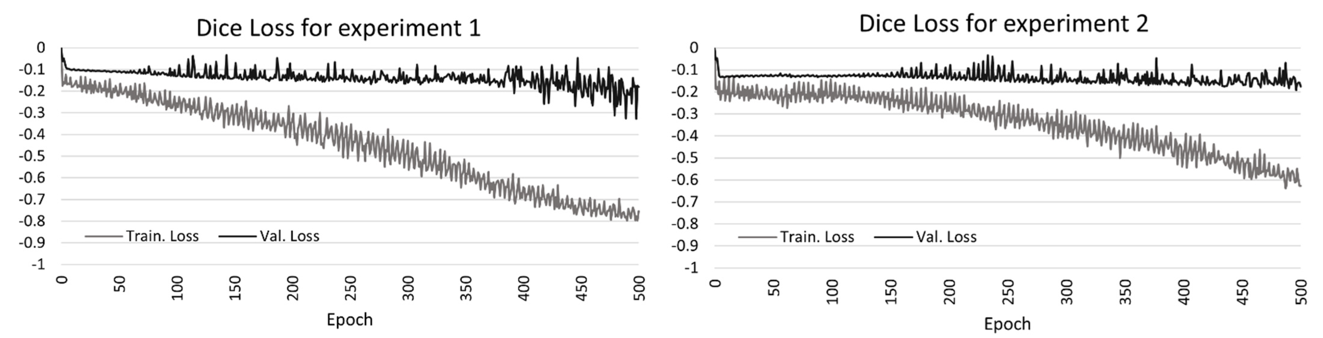
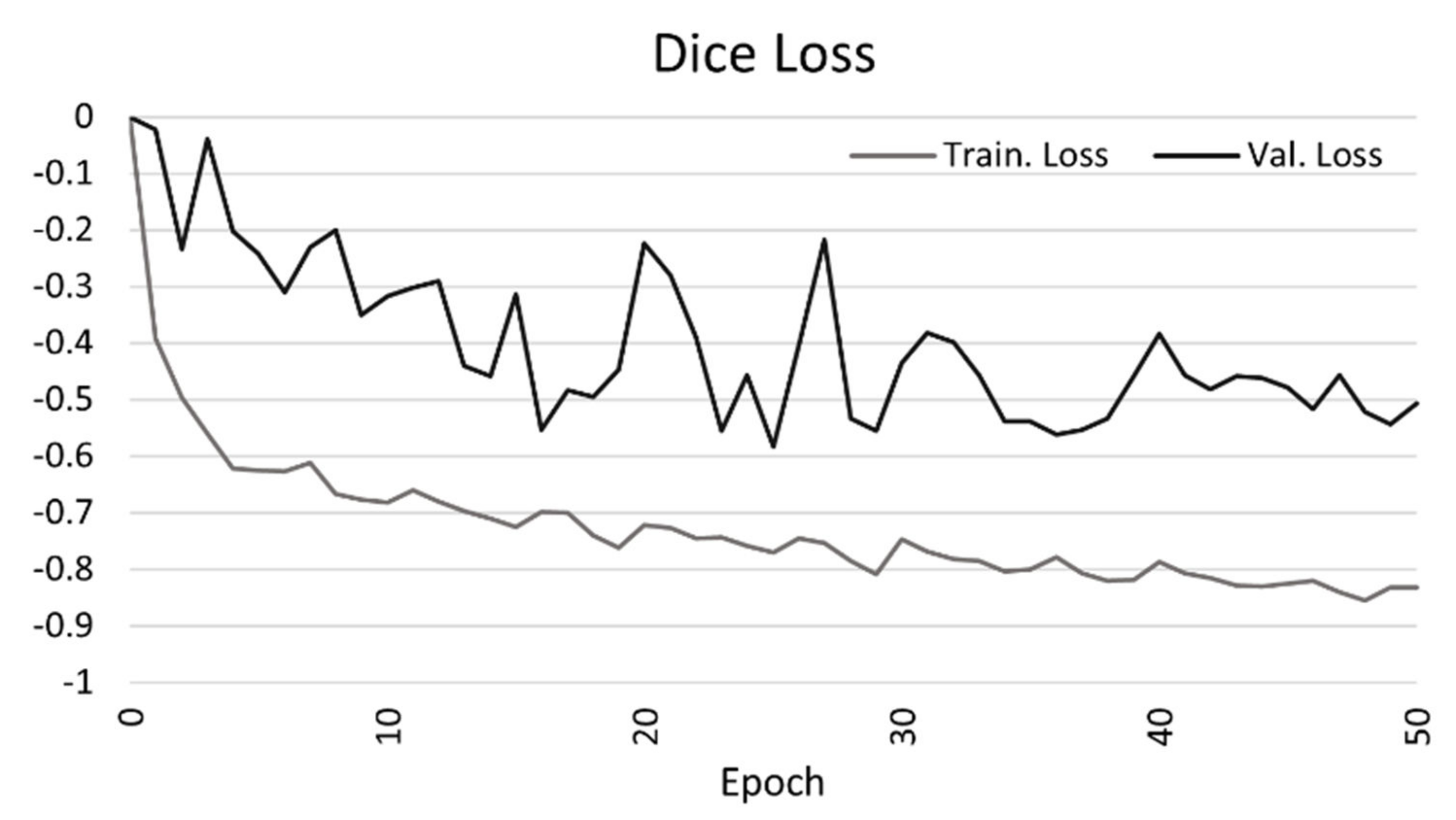
| Train. Dice loss | −0.7771 | −0.6082 | −0.7703 |
| Val. Dice loss | −0.3274 | −0.1917 | −0.5840 |
| Train. Binary accuracy | 0.9817 | 0.9633 | 0.9442 |
| Val. Binary accuracy | 0.9427 | 0.9270 | 0.9085 |
| Train. IoU | 0.4744 | 0.4753 | 0.5835 |
| Val. IoU | 0.4675 | 0.4723 | 0.5141 |
| UOS Experiment 1 | UOS Experiment 2 | ||||
|---|---|---|---|---|---|
| UOS (km2) | Non-UOS (km2) | UOS (km2) | Non-UOS (km2) | ||
| OSM | UOS (km2) | 5.555 | 11.447 | 11.456 | 5.547 |
| non-UOS (km2) | 7.242 | 446.073 | 33.214 | 420.101 | |
| Result | |||
|---|---|---|---|
| LAS (km2) | Non-LAS (km2) | ||
| OSM | LAS (km2) | 38.786 | 30.537 |
| non-LAS (km2) | 22.910 | 378.015 | |
Publisher’s Note: MDPI stays neutral with regard to jurisdictional claims in published maps and institutional affiliations. |
© 2022 by the authors. Licensee MDPI, Basel, Switzerland. This article is an open access article distributed under the terms and conditions of the Creative Commons Attribution (CC BY) license (https://creativecommons.org/licenses/by/4.0/).
Share and Cite
Verde, N.; Patias, P.; Mallinis, G. A Cloud-Based Mapping Approach Using Deep Learning and Very-High Spatial Resolution Earth Observation Data to Facilitate the SDG 11.7.1 Indicator Computation. Remote Sens. 2022, 14, 1011. https://doi.org/10.3390/rs14041011
Verde N, Patias P, Mallinis G. A Cloud-Based Mapping Approach Using Deep Learning and Very-High Spatial Resolution Earth Observation Data to Facilitate the SDG 11.7.1 Indicator Computation. Remote Sensing. 2022; 14(4):1011. https://doi.org/10.3390/rs14041011
Chicago/Turabian StyleVerde, Natalia, Petros Patias, and Giorgos Mallinis. 2022. "A Cloud-Based Mapping Approach Using Deep Learning and Very-High Spatial Resolution Earth Observation Data to Facilitate the SDG 11.7.1 Indicator Computation" Remote Sensing 14, no. 4: 1011. https://doi.org/10.3390/rs14041011
APA StyleVerde, N., Patias, P., & Mallinis, G. (2022). A Cloud-Based Mapping Approach Using Deep Learning and Very-High Spatial Resolution Earth Observation Data to Facilitate the SDG 11.7.1 Indicator Computation. Remote Sensing, 14(4), 1011. https://doi.org/10.3390/rs14041011