Article

Time Series Analysis of Landsat Data for Investigating the Relationship between Land Surface Temperature and Forest Changes in Paphos Forest, Cyprus

by
Vassilis Andronis
1,*,
Vassilia Karathanassi
1,
Victoria Tsalapati
1,
Polychronis Kolokoussis
1,
Milto Miltiadou
2 and
Chistos Danezis
2
1
Laboratory of Remote Sensing, National Technical University of Athens, 9 Heroon Polytechniou Str. Zographos, 15780 Athens, Greece
2
Eratosthenes Centre of Excellence, Civil Engineering and Geomatics, Cyprus University of Technology, Lemesos 3036, Cyprus
*
Author to whom correspondence should be addressed.
Remote Sens. 2022, 14(4), 1010; https://doi.org/10.3390/rs14041010
Submission received: 10 December 2021 / Revised: 9 February 2022 / Accepted: 16 February 2022 / Published: 18 February 2022
(This article belongs to the Special Issue Big Earth Observation Data Analysis for Environment Monitoring)

Abstract

:
This study aims to investigate how alternations of the land surface temperature (LST) affects the normalized difference vegetation index (NDVI) in Paphos forest, Cyprus, using Landsat-5 and Landsat-8 imagery for the time periods 1993–2000 and 2013–2018, respectively. A total of 262 Landsat images were processed to compute the mean monthly NDVI and LST values and create a time series. Using the Cook’s distance, the effect of missing values in the analysis of the time series were examined. Results from the cross-correlation and cross-variograms, decomposition model, and the BFAST algorithm were compared to produce reliable conclusions on forest changes and satellite, meteorological, and environmental data were combined to interpret the changes that occurred inside the forest. The decomposition analysis showed a decrease of 2.7% in the LST for the period 1993–2000 and an increase of 4.6% in the LST during the period 2013–2018. The NDVI trend is negatively correlated to the LST trend for both time periods. An increase in the LST trend was identified in November 1998 as well as in the NDVI trend in October 1994 and May 2014 that was caused by favorable climatic conditions. An increase in the NDVI trend from May 2014 to December 2015 may be related to reduced pityocampa attacks. An abrupt decrease was detected in December 2015 that was probably caused by the locust invasion that occurred in the island earlier that year. A positive correlation appears for LST and NDVI variables for time lags 4, 5, 6, 7, and 8 months. Overall, it was shown that LST and NDVI analysis is very promising for identifying potential forest decline.

Graphical Abstract

1. Introduction

Land surface temperature (LST) is an important climate related parameter which affects the vegetation and biodiversity in an ecosystem. It has, therefore, been recognized as an essential environmental factor for monitoring the resilience of our planet [1]. It is systematically measured by satellite sensors and estimated from TOA brightness values of the infrared spectral bands [1,2]. LST affects the partition of energy between the ground and photosynthesizing chlorophyll and determines the surface air temperature [3,4]. It further influences the thermal environment locally [5,6]. It is observed that LST changes could be abnormal in some areas [7], resulting into droughts, increased frequency of fires, but simultaneously more rainfall and severe storms. LST and other parameters such as the normalized difference vegetation index (NDVI) or bare soil index (BSI) have been mostly studied in relation to urbanization [8,9]. Several studies have been conducted to analyze how changes in LST affect the variability of the microclimate of an area, the phenological cycle of vegetation [5,6], the agricultural production [10], and the land cover changes [11] using time series analysis of data. It has been observed that LST in subtropical and mid-latitude climates (between 30° and 45° latitude) is inversely proportional to the vegetation or tree cover of an area [12,13,14,15]. Relevant research showed that LST and air temperature is reduced by the existence of forests in Europe. The LST reduction effect decreases while the latitude and longitude increase. This has as a consequential warming effect in northeastern Europe [16]. Related work also exists on the evaluation of the relationship between different vegetation indices and LST [15,17], pointing out the negative correlation between LST and NDVI.
The need for products with higher spatial resolution has also led to the release of Landsat products, which have a long and consistent presence in the field of remote sensing, with a spatial resolution of 60–120 m in the TIR region and a time coverage of 16 days [18,19]. Studies with Landsat data showed that mountainous areas are sensitive to rising temperatures, making them vulnerable to climate change [11,12]. Moreover, Landsat data have been used to explore the correlation between LST and vegetation indices during the hot summer period of the year for understanding the effects of LST changes on vegetation. For example, regarding African forests, a study [20] has shown that high temperature areas are mostly barren in contrast to lower temperature areas confirming the negative correlation between NDVI and LST values.
As there is a trade-off between the spatial and temporal resolution of satellite data, time series that are produced by satellite data with high spatial resolution are often sparse over the investigation period. Disturbance factors, such as cloud coverage, aerosols, and systematic sensor errors aggravate the problem of reduced temporal resolution that is crucial for time series analysis [21,22]. Therefore, it is required to interpolate and smooth the values of time series to fill the gaps of the missing values. Here, it worth highlighting that previous works have shown that the Kalman filter produces appropriate and efficient values compared to other interpolation methods [23,24,25].
Furthermore, for analyzing the impact of climate change in forests, data analysis methods have been conducted for estimating changes in the LST trend and identifying correlation points with NDVI trend parameters [26,27]. A trend can be provided by decomposition, a state-of-the-art technique, which analyzes data in the trend, seasonality, and random noise components, to isolate the overall trend, identify any seasonal characteristics, and remove the disturbance factor [28]. Decomposition is usually used for extracting the seasonal relationship with a long-term change for two parameters, e.g., for arable land and urban areas [21].
Multiple approaches have been proposed for tackling decomposition [29,30]. For example, classical decomposition of time series data is either an additive or multiplicative model where all the components are integrated together in an additive or multiplicative phase [31]. Alternatives to the classical approach include X11 Decomposition, which creates a trend-cycle for all the observations and allows the seasonal component to change slowly [32], but it is not robust to outliers. Therefore, researchers introduced the Loess method for estimating linear and nonlinear relationships [33]. State-of-the-art algorithms include trend vegetation analysis for NDVI time series that are based on the BFAST algorithm (breaks for additive season and trend) [34] and a wavelet transform (MRA-WT) [35]. The latter integrates the decomposition of time series with other methods for detecting and characterizing change within a time series. It was used to detect significant changes in the trend and seasonal component of the time series [27].
The main goal of this work is to better understand the effects of LST changes on the forest of Paphos, Cyprus, using NDVI as an indicator of forest degradation. To this end, time series analysis of Landsat data for the period 1993–2018 was carried out. Due to the availability of Landsat data, the time period of the analysis was divided into two district time periods. This division revealed the hidden state of each time period and highlighted micro-changes, which most probably would have not been detectable to that extend if a large continuous time series was processed. It is worth noting that, for each time period, the number of LST and NDVI samples was statistically enough. In this study, the observed LST changes were interpreted with supplementary use of meteorological data, such as aerial temperature and precipitation, taking into account that, in general, air temperatures above a surface reflect the same trends as the ground surface temperatures, while the ground temperatures are likely to be more extreme. Interpretation of the response of NDVI to LST changes was also supported by the meteorological data. Environmental factors such as insect invasion and pest attacks, could be identified through unusual and abrupt NDVI changes in the study area.
For handling missing values in the produced time series, the Kalman smoothing filter [23,34] was evaluated and compared to regression analysis using the Cook’s distance and Hat matrix. Annual density plots helped initial observations on the completed LST and NDVI time series, while the additive seasonal decomposition model and the BFAST algorithm served as tools for analyzing the time series and detecting breakpoints. The influence of points with significant Cook’s distance on the trend component was examined. The interpretation of abrupt changes in LST and NDVI trends identified the parameters that caused changes in the forest of Paphos, while correlation analysis and cross-variograms of the LST and NDVI variables indicated their convergences and divergences in time. Finally, extensive analysis of the residuals substantiated the choice of the decomposition model and provided additional information on the potential changes in the forest.
The paper studies the effect of missing values in the analysis of the time series by the utilization of Cook’s distance. It further compares the results from cross-correlation and cross-variograms, as well as the decomposition model and the BFAST algorithm, to produce reliable conclusions on forest changes. Furthermore, it aims to produce meaningful results for the response of vegetation to LST changes and the impact of climatic factors on changes in the Paphos forest, Cyprus, over the last decades. It combines satellite, meteorological, and environmental data to interpret changes in a Mediterranean forest which is under threat due to climate change, as Mediterranean forests are expected to be affected more severely by climate change in comparison to other European regions [36].

2. Study Area

The study area was the Paphos forest in Cyprus (Figure 1), located in the western part of the Troodos mountain range. This is a coniferous forest of 600 km2 including two natural areas and it was selected since it represents an ecosystem of great importance. Additionally, according to a recent survey conducted in Cyprus 38.7% of the participants noticed much to very much and 26.92% moderate degradation on coniferous forest in Cyprus, while 44% believed that conifers are the most affected plant species by climate change [37].
The predominant vegetation species in this forest is the Pinus brutia. In addition, some species of smaller trees and shrubs are an important part of the forest such as the Guercus alnifolia, Arbutus andrachne, Olea europaea, Cistus creticus, Ramnus alaternus, and Guercus coccifera. Remarkable is the riparian vegetation consisting of broadleaves, i.e., Platanus orientalis, Alnus orientalis, Laurus nobilis, Myrtus communis and the bush, Rubus sanctus, which appears independently from the altitude. In addition, especially at low altitudes, fewer tall trees and more small shrubs, phrygana, and herbaceous plants are found. Finally, the Cypriot cedar (Cedrus brevifolia) is found on the slopes of Tripylon from 600 m to 1352 m, along with vegetation species such as Origanum cordifolium, Ranunculus kykkoensis, Onosma mitis, Erysimum kykkoticum, and Arum tupicola [38].
Analysis based on Landsat time series images that characterize the extent and change of forests worldwide [39], showed forest loss in the study area in 2016. Specifically, in the Global Forest Watch’s (GFW) interactive world forest map and tree cover change data (https://glad.umd.edu/projects/global-forest-watch (accessed on 31 January 2022)), mapped a loss of tree coverage that was greater than 30% of the canopy density for an area covering about 0.7% of the study area.
Furthermore, the overall area of the island, including the Paphos forest, faces a problem with locusts [40]. Locust swarms have become endemic since the mid-sixteenth century. For reasons that are not yet fully understood, locusts appear in Cyprus in greater abundance in some years than others. It is also worth noting that attacks of Thaumetopoea pityocampa have been increased in the Mediterranean [41] due to climate change, resulting in a significant reduction in pine growth and some deaths. T. pityocampa attacks are reduced in cases where low temperatures are observed in the autumn months [42].
The climate in the study area is characterized as Mediterranean, with key features of hot and dry summers and rainy but mild winters. The general climatic conditions are affected in summer by the seasonal barometric low, which is centered in southwest Asia and causes high temperatures and clear weather, while in winter conditions are affected by small successive recessions, from west to east, which are responsible for a large percentage of annual precipitation. In summary, the main climatic characteristics of Cyprus are the following: the ‘normal’ average annual rainfall is 503 mm and the average temperatures range from 22 °C to 29 °C, in the summer months and from 3 °C to 10 °C, in the winter [38]. The ‘normal’ rainfall is referred to as the mean rainfall value of historical data.
The years 1992, 1993, and 1997 were the coldest years of the decade 1990–2000 in the forest region, with a mean aerial temperature of 16.97 °C, 18.16 °C, and 17.79 °C, respectively. Moreover, according to data that were provided by the Department of Meteorology of Cyprus, in 1992 the rainfall was 637 mm, an increase of 27% from the “normal” in the study area. In 1993 it was 509 mm which also increased by a small percentage of 1.8% of the ‘normal’ rainfall. Increased annual rainfall is also observed for the year 2014 (562 mm) in comparison to 2013 (315 mm) and 2015 (309 mm), respectively. The autumns in 2013 and 2014 were colder (14.70 °C and 13.35 °C, respectively) than usual, where temperatures greater than 15 °C are typically observed.
According to the analysis of the Department of Meteorology of Cyprus, the temperature in the wider area of Cyprus has been characterized by significant fluctuations and trends. Regarding the temperature, during the 20th century its trend was upward and its mean growth rate was 0.01 °C/year [43]. In particular, for the period 1976–1998 it was proven that the mean rate of temperature increase was 0.035 °C/year in urban areas and 0.015 °C/year in the open air. Additional processing of the meteorological data for the period 1991–2007 showed that the mean annual temperature was 17.7 °C, which exceeded the corresponding temperature (17.2 °C) of the period 1961–1990 by 0.5 °C. From regional climate models (RCMs) it has been predicted that during the period 2021–2050 in the areas of Troodos mountain range, the maximum temperature is expected to increase by 1.9 °C [43].

3. Materials and Methods

3.1. Data

A total of 186 Landsat-5 satellite images were initially downloaded for the period 1993–2011 and 76 Landast-8 satellite images for the period 2013–2018. The Landsat products were projected on the reference coordinate system WGS 84/UTM zone 36N.
The aerial temperature data were provided from the database of the Department of Meteorology in Nicosia, Cyprus. These data were recorded at 10 am (local time) in Celsius degrees at the climatic station named “Cross of Psoka”, which has a latitude of 35°01′29.52″ N, a longitude of 32°37′50.78″ E, and an altitude of 824 m. The average monthly value from these data was used from the time period January 1992 to April 2016.
Additionally, the daily and mean annual precipitation data were provided from the database of the Department of Meteorology in Nicosia, Cyprus for the period 1990–2020.

3.2. Methods

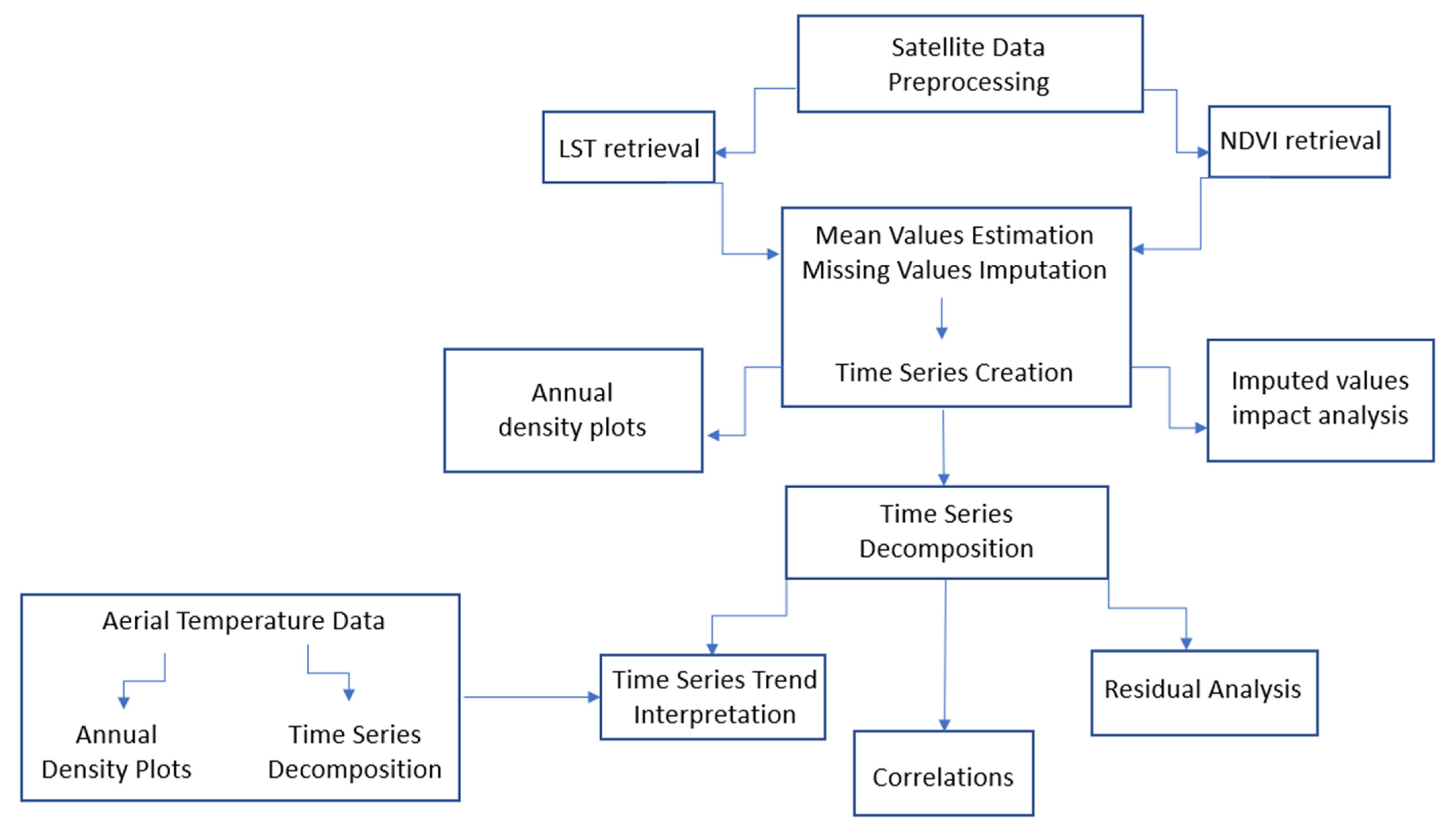
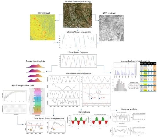
The satellite image processing and time series analysis were employed for the needs of the study. The R programming language was used for the time series analysis steps. Figure 2 presents the steps of the methodology.
The satellite images that were acquired by optical sensors usually contain noise (e.g., clouds and aerosols). Thus, the fmask algorithm [22] was used to remove the cloud cover areas from the Landsat imagery. The algorithm uses the v3 ASTER Global Digital Elevation Model (ASTER GDEM) to normalize the thermal Landsat bands and data that are provided by the Global Surface Water Occurrence (GSWO). After this process, the final cloud mask is created for each image.
After quality inspection and cloud masking several images were discarded, resulting in a dataset of 125 Landsat-5 images and 60 Landsat-8 images (Level-1 for the thermal bands and Level-2 for multispectral bands). These images covered two time periods, (a) 1993–2000 (staring in March 1993 and ending in February 2000) and (b) 2013–2018 (starting date in April 2013 and ending in March 2018).
To estimate the land surface temperature from the Landsat thermal infrared bands, the method that was described in [17] was followed. The method requires the estimation of the NDVI using the red and near-infrared bands of the multispectral images. The result of the processing was LST and NDVI images for the two time periods: 1993–2000 and 2013–2018.
For each LST and NDVI image, the mean value of the pixels lying within the study area was calculated. In case of two satellite passages per month, one value per month was calculated using the average LST or NDVI value. In the time series, the missing values corresponding to the discarded images were also observed. To address the gaps of the missing values, the Kalman smoothing filter [44] and the moving average (MA) interpolation were applied. Based on the evaluation of the results, the completed datasets by the Kalman smoothing filter, were used for the time series analysis.
Annual density plots of the completed LST and NDVI time series were used to study the effect of missing values on the time-series.
For understanding the effects of the imputed values while analyzing the time series data, the Cook’s distance was calculated which relies on the Hat matrix. The Hat matrix (H), shows the effect of each time series value y (response value) on each fitted value ŷ produced by the Kalman filter, taking into account that ŷ = H × y, where the elements of H are derived by the covariance between the response value and the fitted value, divided by the variance of the former. From the trace of H, the levers describing the effect of each response value on each fitted value for the same observation are found and the high leverage points that influence the regression coefficients of each additive decomposition are found.
The Cook’s distance (D) is a metric that helps us to identify the effect that each time series value has on each fitted value that is generated after applying the Kalman filter, taking into account all observations. The Cook’s distance D i of observation i (for i = 1, …, n) is defined as the sum of all the changes that are produced by the Kalman filter when observation i is removed from it, i.e., in the following equation, j = 1, …ki, k + i …. n.
D i = j = 1 n ( y ^ j y ^ j ( i ) ) 2 p s 2
where p is the number of covariates for each observation and s 2 is the mean squared error of the estimated values. The Cook’s distance is also used to estimate how much the residuals values between the initial observations and estimated values by the Kalman filter would change if the specific observation value indicated by the Cook’s function, was not taken into account [45]. Influential values are not always a problem in case that their removal from the dataset leaves the parameter estimates that we are interested in, essentially unchanged. Thus, in this study, the values with significant Cook’s distance were removed from the time series and estimated using the Kalman filter. The additive decomposition model and the BFAST algorithm, which are described below, were then applied to test whether the influential values changed the results.
The additive seasonal decomposition by moving averages [30,46] is a fast, stable, and consistent way to decompose time series into their components: trend, seasonality, cycle, and randomness. Randomness corresponds to the remaining values (residuals) of the time series, after subtracting the other three components. The approach estimates the values of (Xt) where (t) is a set of consecutive time points, as expressed by the equation of the additive decomposition model:
Xt = Tt + St + Rt
where (Xt) is the data, (Tt) is the trend-cycle component, (St) is the seasonal component, and (Rt) is the residual component, all at period (t).
In this study, decomposition is applied on aerial temperature, LST, and NDVI time series. Decomposition of the aerial temperature time series delineates the “big picture” of temperature changes in the area covering the period from January 1992 to April 2016, and helps the interpretation of LST changes.
Decomposition of LST and NDVI time series was used to understand the response of NDVI to LST changes during the two time periods (1993–2000 and 2013–2018). LST and NDVI trends showed the magnitude of the change in time of the two variables and revealed smooth as well as abrupt changes. The relationships between the LST–NDVI trend lines indicated the systematic impact of LST changes on vegetation.
To cross-check the abrupt changes in the LST and NDVI trend lines, the BFAST algorithm [34] was applied. The algorithm detects statistically significant changes in time series combining change detection with the additive decomposition of the time series. LST changes alone are not enough to interpret abrupt changes of NDVI time series. Climatic factors such as precipitation, and other environmental factors, e.g., insect invasion, may cause changes to vegetation, which are highlighted by abrupt changes in the NDVI trend line.
For validating the assumptions of the additive decomposition model, residual analysis was performed. The residual analysis indicates the suitability of the models, bias in estimations, and potential improvements in model quality. None of the explanatory information should be contained in the residuals, except for the context of randomness. Additionally, residuals should be randomly distributed around the value 0. Residual analysis in this study included (a) the normal Q-Q plot for testing for characteristic departures from normality, (b) residuals versus fits scatter plots to check homoscedasticity, (c) scale-location plots for checking the spread of the residual, and (d) residual leverage plots to indicate points with high leverage. Furthermore, the cross-correlation coefficients were estimated for each month between the LST and NDVI residuals for the 1993–2000 and 2013–2018 time series, to reveal changes in the relationship between the two variables that are not easily interpretable by observing the seasonal graphs.
Analysis of the LST and NDVI time series was completed by auto and cross-correlations. The auto correlation function (ACF) was used to measure the linear relationship between an LST (or NDVI) observation at time t and the observations at previous times. Similarities of the auto correlation functions for the two variables indicated that LST and NDVI time series have similar patterns. Cross-correlations for lags from one to twelve months as well as the cross-variogram of the LST and NDVI parameters were applied to reveal relationships of the NDVI series to past lags of the LST series. Cross-correlations are helpful for identifying lags of the LST variable that might be useful predictors for NDVI.
Interpretation of the satellite time series analysis was supported by aerial temperature data. First order statistics and ergodic mean monthly values were estimated, annual density plots were created, and the additive decomposition model was applied for this purpose.

4. Results and Discussion

4.1. The Effect of Missing Values in the Satellite Time Series

The percentage of missing values was 33% for the LST and NDVI time series for the period 1993–2000 and 25% for the LST and NDVI time series for the period 2013–2018. Especially for the years 1998 and 1995, the missing values present high percentages of the rank of 58.3% and 41.67%, respectively, while for the years 2016 and 2015 the missing values present percentages of the rank of 41.7% and 33.4%, respectively.
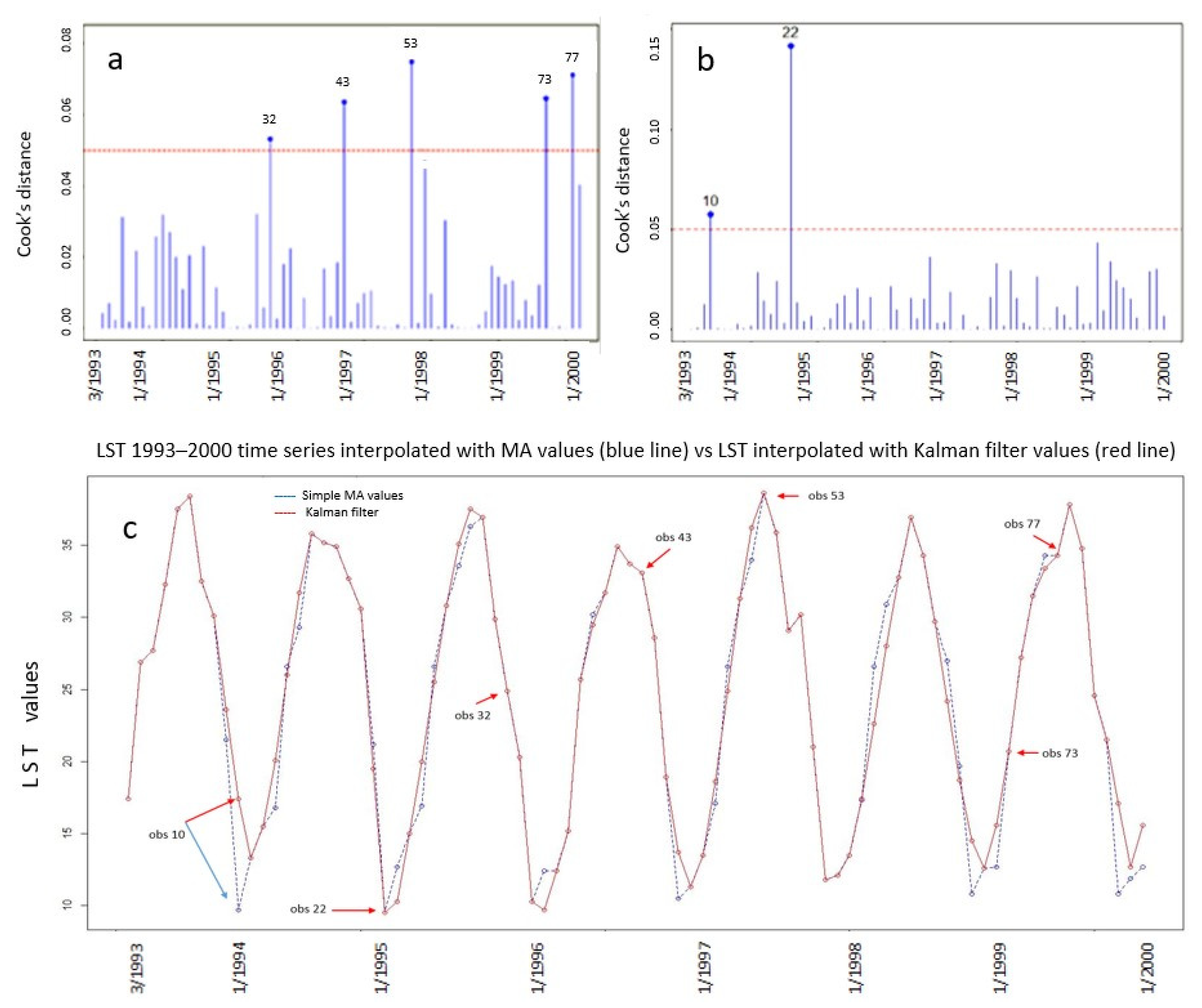
The Kalman filter created much fewer points of influence (Figure 3b) and produced smoother graphs (Figure 3c). In Figure 3b, point 22 that corresponds to December 1994 observation in Figure 3c, appears as a point of influence, with a Cook’s distance of about 0.16 that was much higher than the upper limit of the confidence level of 0.05 that is represented by the red line in the chart. We should note that observations 21 and 23 are missing values in the time series. Therefore, the influence of observation 22 on the Hat matrix was also exacerbated by the discontinuity and instability of neighboring values. Moreover, observation 10 corresponds to the LST value of December 1993 and it is a missing value in the original time series data. Here, the influence of observation 10, is also graphically evident in Figure 3c, where there is a noteworthy movement of point 10 after the application of the Kalman filter in relation to the MA interpolation.
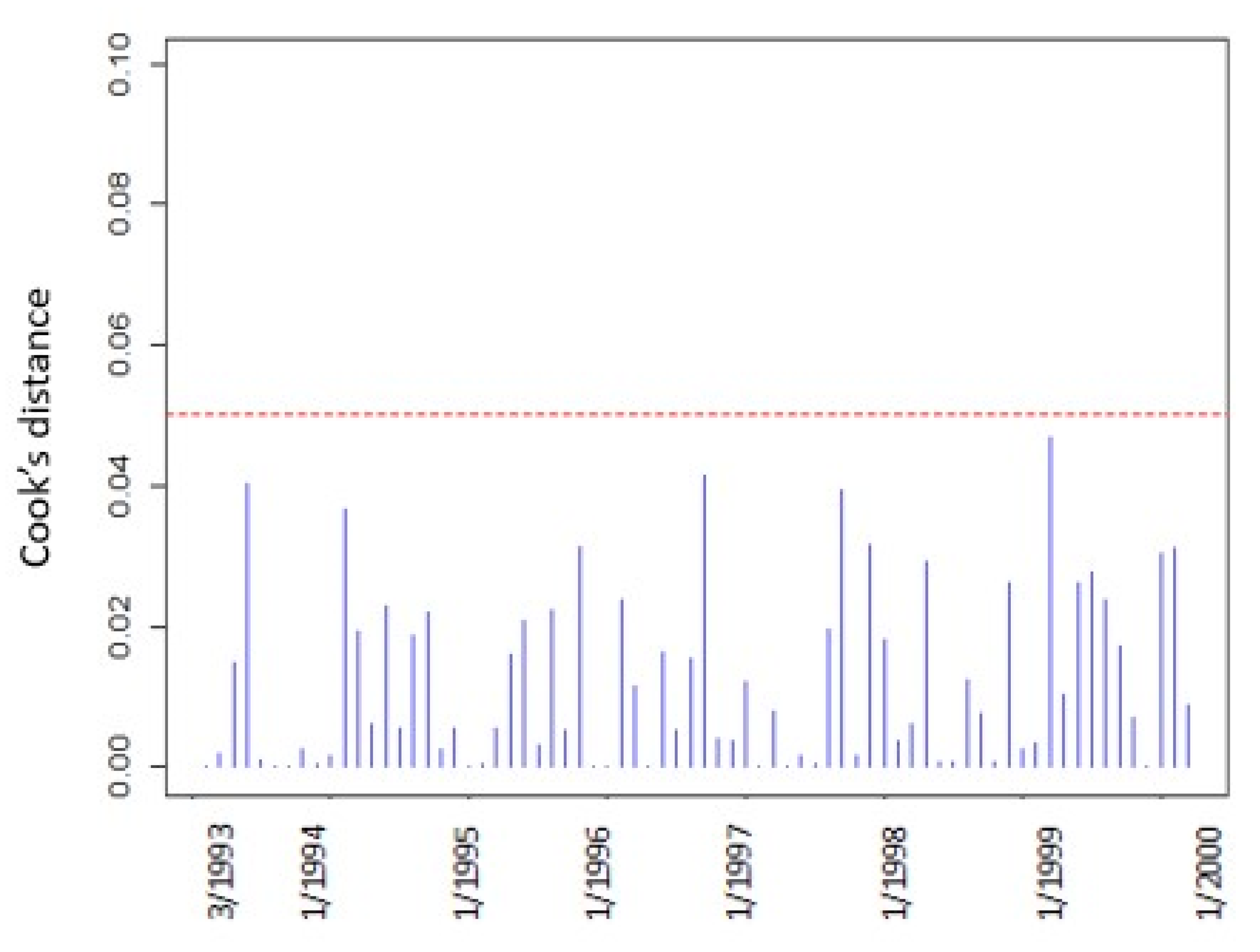
In Figure 3a, points 32, 43, 53, 73, and 77 that correspond to the LST observations for October 1995, September1996, July 1997, March 1999, and July 1999, respectively, appear as points of influence and they are significantly higher than the confidence level of 0.05. These points are also marked with arrows in Figure 3c and they do not appear to show a significant change in the graphical representation of the time series, so they do not appear to have any interest in contrast to points 10 and 22 which affect their neighboring points. Points 10 and 22 were removed from the original time series and were estimated using the Kalman filter. The Cook’s distance was derived from the updated time-series (Figure 4) and it showed no influential points.

4.2. Annual Density Plots and First Order Statistics

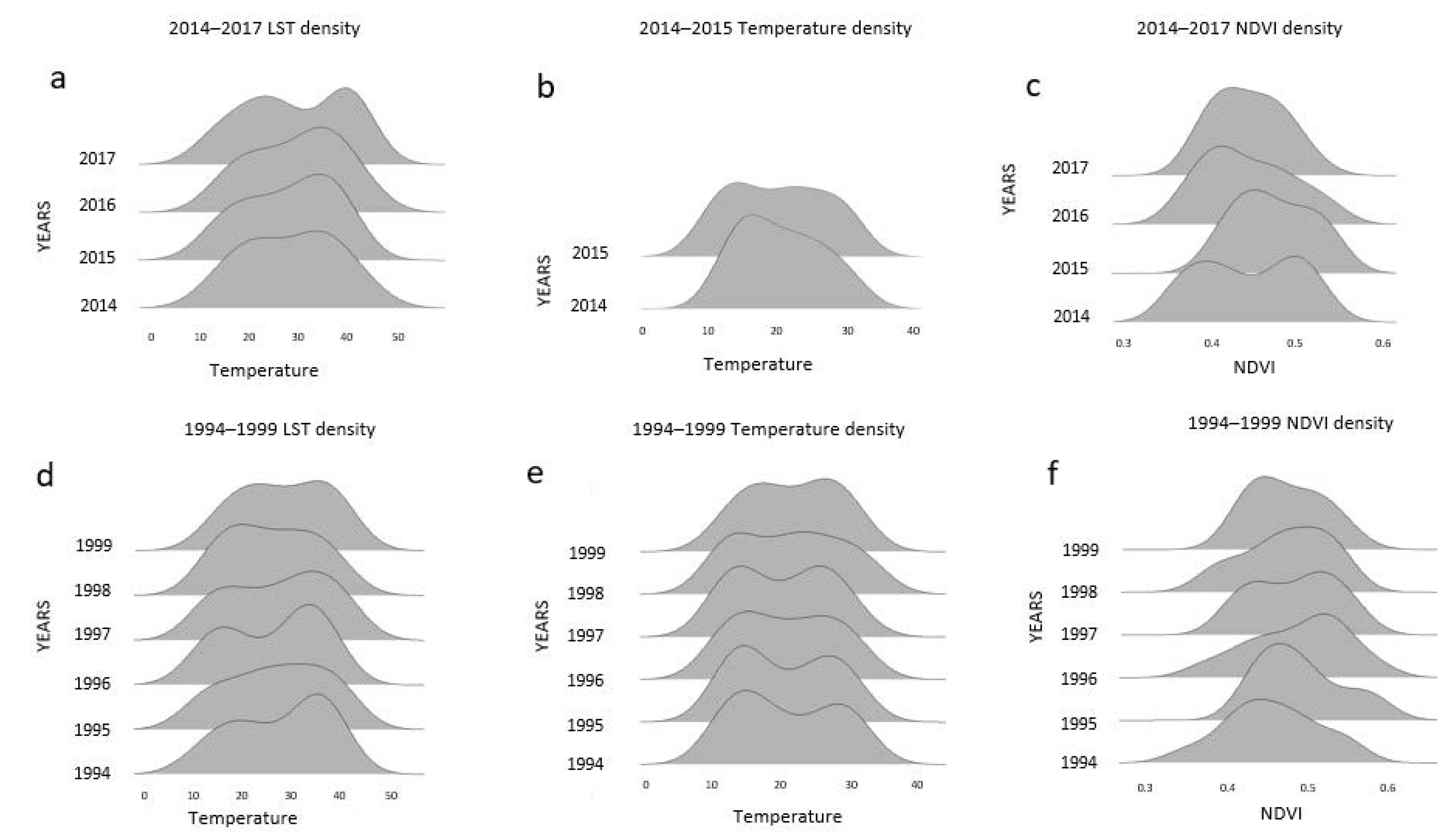
For observing the yearly distribution of LST, NDVI, and aerial temperature data, annual density plots were produced (Figure 5). Density plots were created for the years 1994–1999 for the LST, NDVI, and aerial temperature, for the years 2014–2017 for the LST and NDVI, and for the years 2014–2015 for the aerial temperature, since only for these time periods, data for all the months were available.
As shown in Figure 5b,e, the annual distributions of the aerial temperatures were a mixture of normal distributions. The distributions of most years presented two peaks with almost equal accumulations, one in the low and one the high temperatures. Τhe forest ecosystem seems to contribute to this balance of temperatures. Only for the years 1996 (Stdev 7.76 that is the minimum for the period 1994–1999) and 2014 (Stdev 6.58 that is the minimum for the period 2013–2016) were the distributions of the temperatures presented as one peak.
The density plots of 1994–1999 LST time series (Figure 5a,d) shows some interesting points. The year 1995 (Figure 5a) presents a graph of rather normal distribution with a large dispersion while for the other years, the graph shows a mixture of two distributions with displacement to higher temperatures. For the year 1998, the mixture is almost balanced. The form of these plots rather reflects the effect of the Kalman filter in the time series because for the years 1998 and 1995, the imputed values present high percentages, of the rank of 58.3% and 41.67%, respectively, and thus the respective distributions present smooth curves with a not well-defined peak. This remark is also confirmed in the plots of the LST time series 2014–2017 (Figure 5d), where in the years with the most imputed values (41.7% in 2016 and 33.4% in 2015) the density plots showed greater smoothing.
Most of the NDVI density plots showed a mixture of distributions that is homogenized as a simple distribution. Exceptions are the density plots of the years 1997 and 2014 which present two peaks.
First order statistics of the time series are shown in Table 1. For their comparison, the total sample of 292 meteorological observations were adjusted over the LST time series. We observed that the aerial temperatures in the forest area showed an almost constant mean negative deviation of about 6.50 degrees from the respective LST mean. A similar deviation is also reported in [47].
We observed that the mean values of the LST and aerial temperature for the second time period presented an increase in relation to those of the first time period. However, because the two LST time series were derived from data that was captured in slightly different spectral regions, hereinafter we will avoid their direct comparison.

4.3. Remarks on Time Series Trends

4.3.1. Aerial temperature

According to the additive decomposition model, the linear equation that describes the trend component is y = 18.244 + 0.0031197x. By examining the whole air temperature time series (Figure 6b), no significant variations between the yearly values of aerial temperatures were identified. However, with a closer look at the diagram of the ergodic mean (Figure 6a), an upward trend appears. This observation agrees with the upward trend of the order of 0.3%, that is indicated by the coefficient of the trend component equation. The observed trend is aligned with the analysis of the Department of Meteorology of Cyprus [43] (Section 2).

4.3.2. LST

In the LST 1993–2000 time series, the trend line (y = 24.818 − 0.026929x) had a negative slope of 2.7%, (Figure 7a). This can be justified by the aerial temperatures. The years 1992, 1993 and 1997 were the coldest of the decade 1990–2000 (Section 2). Moreover, in 1992, the rainfall was significantly higher in relation to the normal rainfall in the study area, while 1993 also presents a slight increase in relation to the normal rainfall (Section 2).
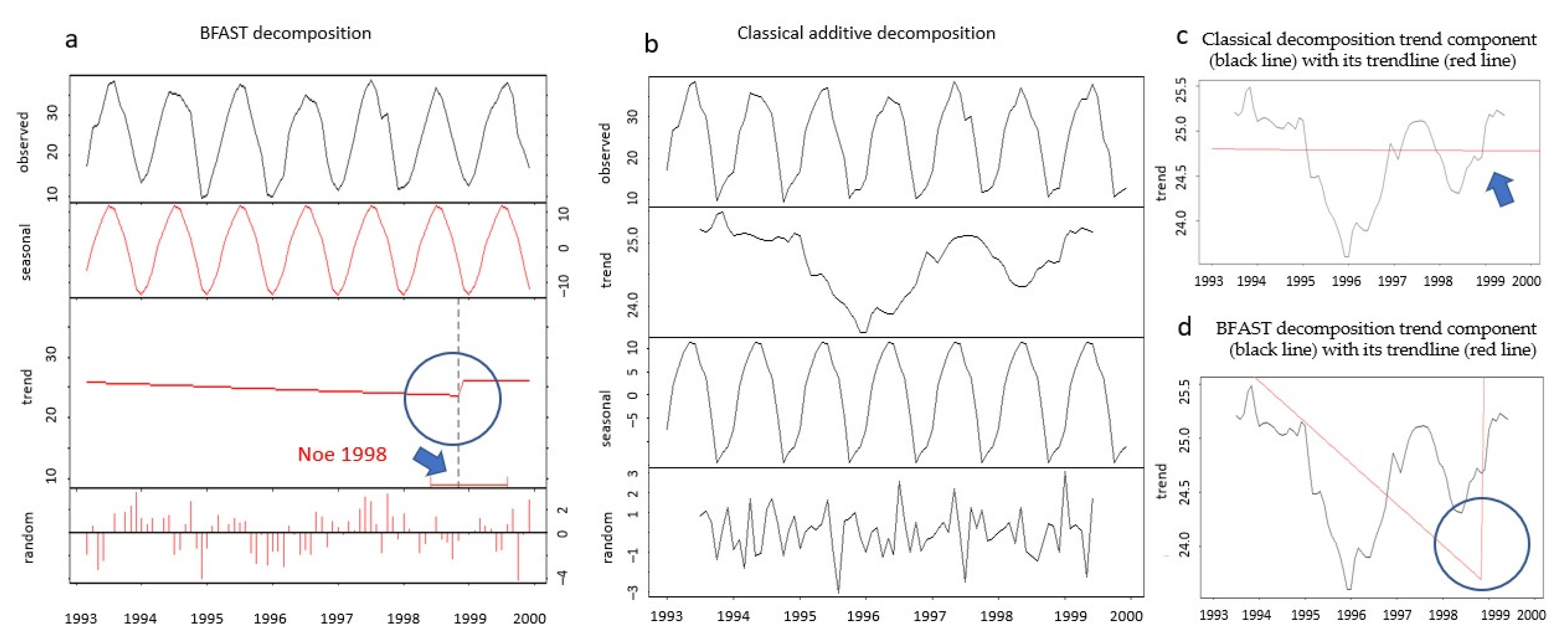
In the LST 1993–2000 time series, an unusual increase of the LST trend component was detected by the BFAST algorithm in November 1998 (Figure 8a,c,d), which is marked with an arrow in Figure 8a. This was a point marking a significant increase in the trend line. This point coincides with point 2 in (Figure 7a). For interpreting this result, we examined the average annual LSTs for the years 1998 and 1999. It was observed an average of 23.73 °C for 1998 which significantly increased to 26.09 °C for the year 1999. Moreover, an increase was observed in the average annual aerial temperatures for the years 1998 and 1999, where air temperature from 19.00 °C rose to 19.46 °C. Point 1 in (Figure 7a) that corresponds to August 1995 was not identified as a point of statistically significant change by the BFAST algorithm. By examining the LST values, we observed that the years 1994, 1995, and 1996 present an average of 25.40 °C, 24.71 °C, and 23.93 °C, respectively, showing a rather smooth decrease in the trend. The BFAST algorithm, therefore, conferred satisfactory results, indicating that further analysis of the trend line after the decomposition was required to draw conclusions about the statistically significant points of the LST. In the LST 2013–2018 time series, the trend line had a clear upward slope (y = 23.17 + 0.046534x) of 4.6%, (Figure 7b), while it does not present significant changes. The BFAST algorithm also did not reveal signs of significant changes (positive or negative).
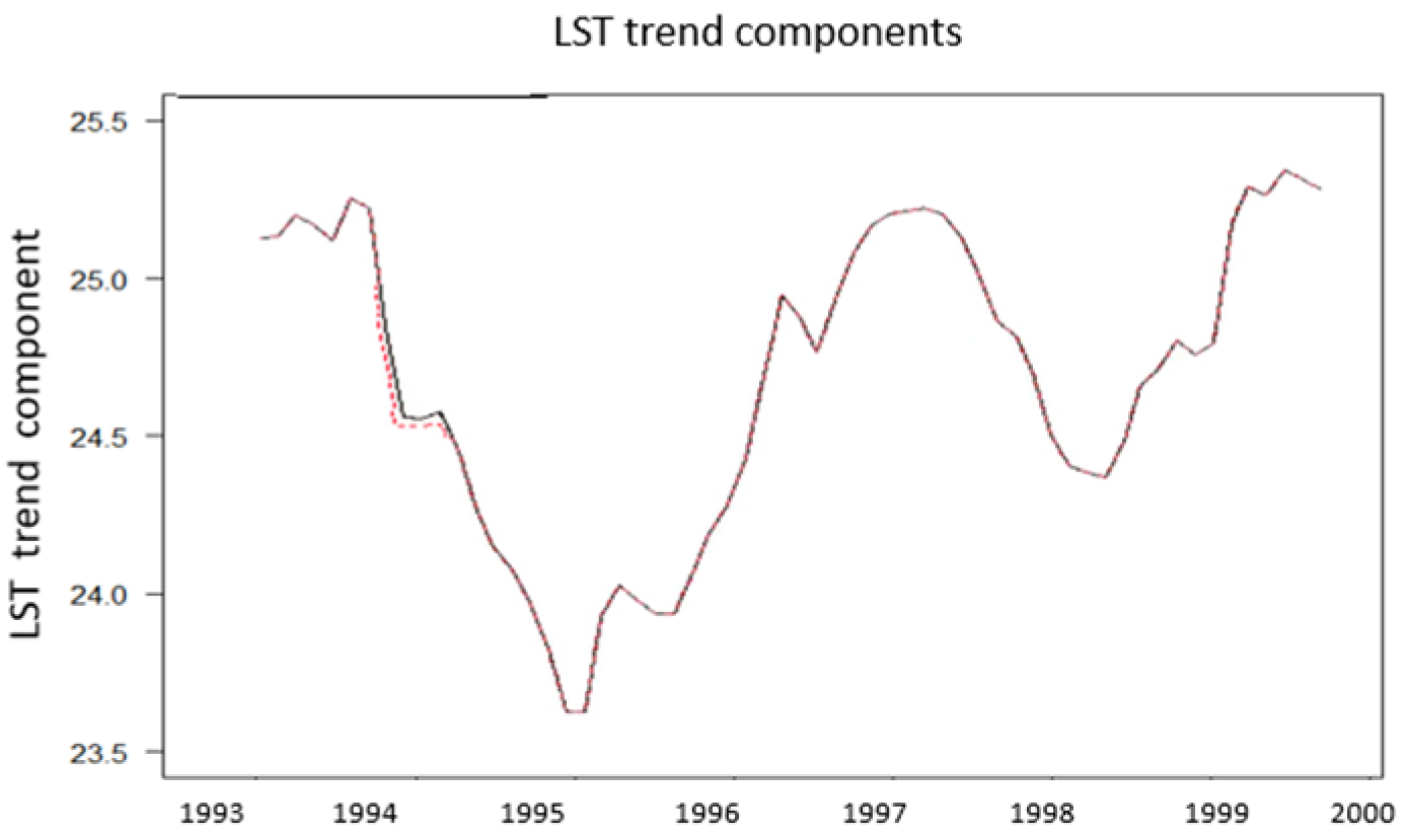
The additive decomposition model and the BFAST algorithm were also applied on the LST time series, in which the values of the influential points 10 and 22 were replaced by new values that were calculated by the Kalman filter (Figure 9). The results showed that influential points changed locally and very slightly the trend of the time series. The break points that were indicated by the BFAST algorithm were the same.
In the LST 2013–2018 time series, the trend line had a clear upward slope (y = 23.17 + 0.046534x) of 4.6%, (Figure 7b), while it did not present significant changes. The BFAST algorithm also did not reveal signs of significant changes (positive or negative).

4.3.3. NDVI

In the 1993–2000 NDVI time series, an upward trend of 0.02% was observed (y = 0.44164 + 0.00026747x), (Figure 10a). The mean value of the NDVI index during this period was 0.45, while an unexpectedly sharp increase in the trend component that occurred in October 1994 should not be ignored. In the NDVI 2013–2018 time series, there was a downward trend (y = 0.56516 − 0.00033242x) of the rank of 0.03% (Figure 10b). During this period, the mean value of the NDVI was 0.56 but it should be noted that the NDVI values that were derived from Landsat 8 images are known to be higher than those of Landsat 5 [48,49], so these mean NDVI values are not easily compared. Regarding the 2013–2018 NDVI time series, two interesting changes were identified in the trend component: one in May 2014 and one in December 2015.
The BFAST algorithm detected statistically significant changes in the NDVI time series components (Figure 11). In the NDVI 1993–2000 time series, a significant change in trend was identified in October 1994 (Figure 11a–c). October is the month when the evergreen shrubs and geophytes reflect enough in the infrared bands and act competitively on trees. Usually, high NDVI values are observed during this month due to the growth of shrubs and geophytes. The high precipitation levels in the years 1992 and 1993 probably contributed to the increase of shrubs in the forested area which it was pronounced by an abrupt increase of the NDVI values in October 1994. After that, the NDVI values were kept almost constant with a slight decline which shows the climatic impact on the vegetation.
For the NDVI 2013–2018 time series (Figure 11d–f), the BFAST algorithm detected two points of unusual changes in the vegetation. One concerned the period around May 2014, where a significant increasing trend of NDVI was observed until December 2015. This may be linked to reduced act of T. pityocampa due to low temperatures in the autumn months. Specifically, in autumn 2013 the average temperature was 14.70 °C, in autumn 2014 the average temperature dropped to 13.35 °C, while in autumn 2015 the average temperature rose to 15.62 °C. Moreover, a significant amount of rainfall in May 2014 (49.2 mm) favored the growth of vegetation. The increase of the mean LST from 22.9 °C (April 2014) to 27.6 °C (May 2014) and the mean aerial temperature from 17.2 °C (April 2014) to 20.1 °C (May 2014), also created favorable conditions for vegetation.
The second turning point of the trend was identified in December 2015 (Figure 11d). There was a noticeable decrease after December 2015 which agrees with the forest loss in the study area that took place in 2016 and was identified and mapped by the Global Forest Watch’s (GFW) interactive world forest map and tree cover change data. This abrupt decrease could also be related with the dates that a locust invasion hit the Eastern wider region of Europe in 2015, which was also a blow for the islands in the southern part of the Mediterranean.

4.4. LST and NDVI Correlations

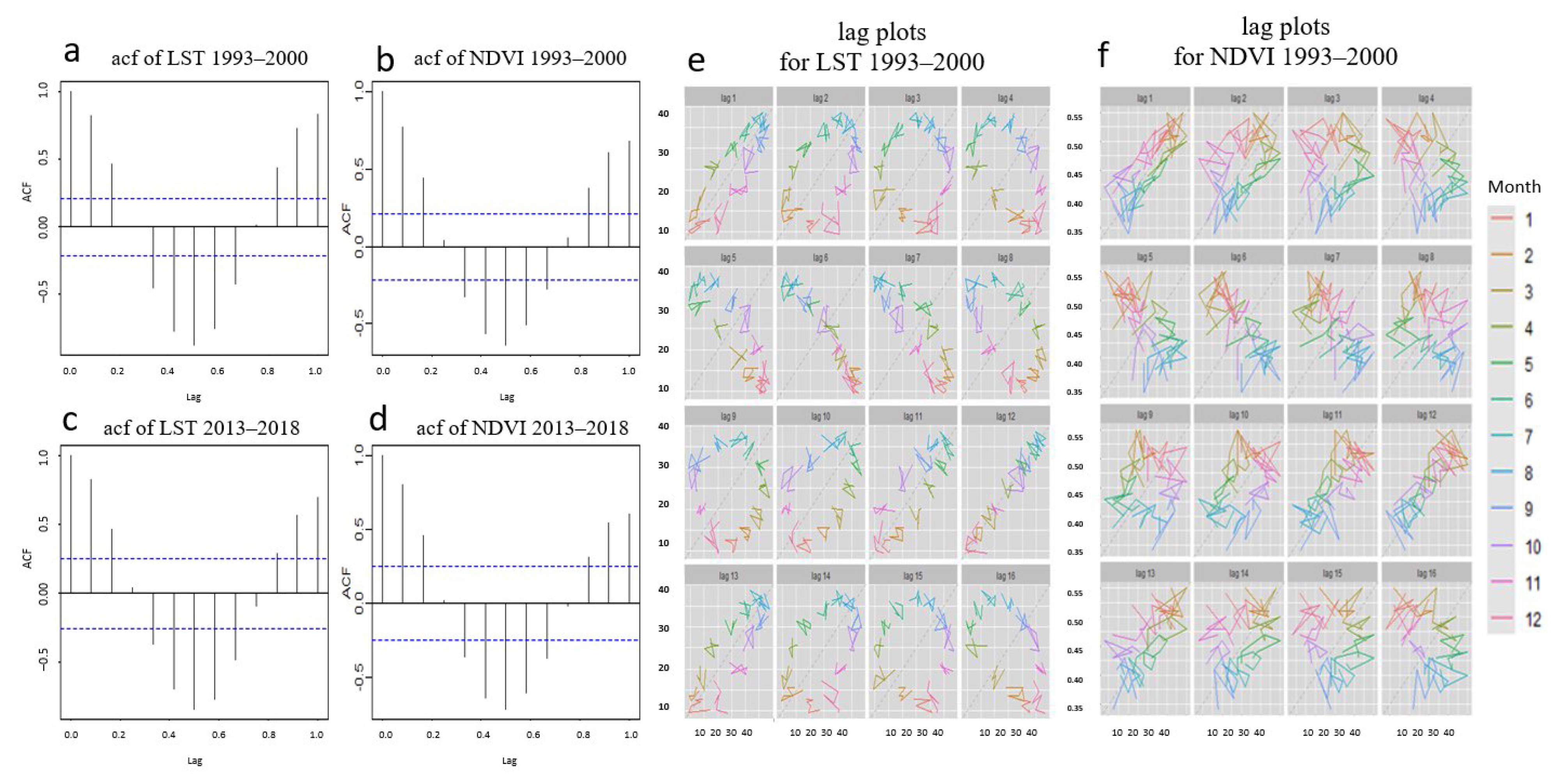
For the LST and NDVI 1993–2000 time series, autocorrelation function (ACF) (Figure 12a,b), shows a strong negative correlation on the sixth month. This result is also confirmed by the lag plots (Figure 12e,f), where the colors are indicative for the value of the variable on the y-axis. The relationship was very positive for the lag of 12 months (lag 12 in Figure 12e), reflecting the strong seasonality in the data while there was a strong negative relationship for the lag of six months (lag 6 in Figure 12e). It was observable that the negative correlation starts from lag 5 and lasts until lag 7. Regarding the 2013–2018 LST and NDVI time series, the results are very similar (Figure 12c,d).
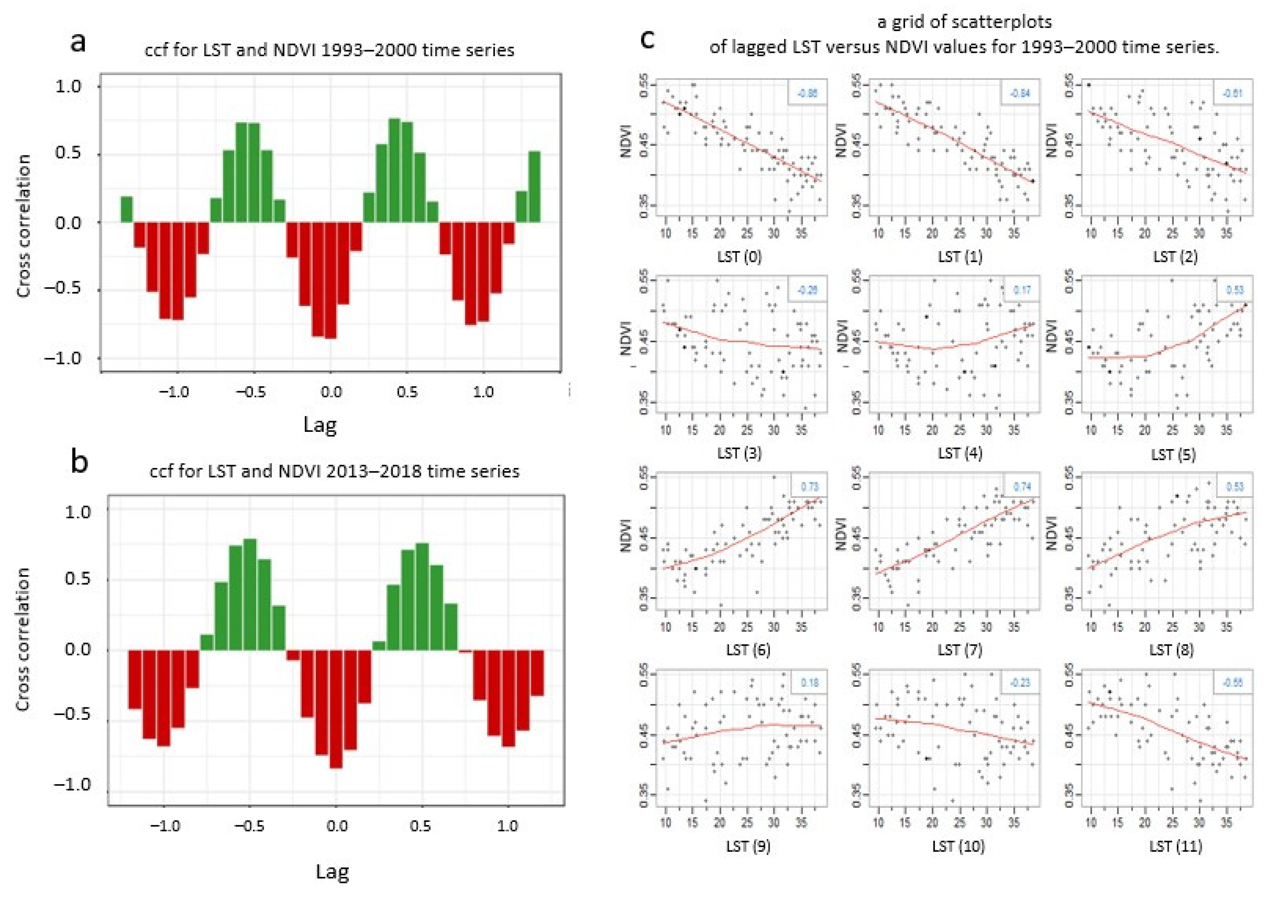
Moreover, a cross-correlation function (CCF) was calculated for the LST and NDVI for the time period 1993–2000, after standardizing their samples [50] to ensure uniformity and consequently comparability. From the correlation function, a strong negative correlation up to the first three lags was observed (Figure 13a,c), then the correlation was reversed to positive for the following three lags (Figure 13a,c). When the lag plot produces a linear graph, it means that correlation is present in the data. The slope of the line of the datasets determines whether there is a correlation, and the direction of the slope indicates whether the correlation is positive or negative. If more data are concentrated on the diagonal in lag plot, it means there is a strong correlation, as in Figure 13c, lag (0), lag (−1), lag (−2), lag (−6), and lag (−7).
Regarding the 2013–2018 LST and NDVI time series (Figure 13b), strong negative cross-correlations were present for the first two lags, which is in line with the result of the 1993–2000 time series. The dominant positive cross-correlation appeared for lag (6), suggesting that a high mean LST value was associated with the occurrence of a high mean NDVI value with six months difference.
Additionally, the cross-variogram of the LST and the NDVI variables was calculated to correlate the LST and NDVI values in different lags. A range of influence of about 5.5–6.5 months was observed for the 1993–2000 time series and a positive correlation appeared for lag (4), lag (5), lag (6), lag (7), and lag (8), which then became negative (Figure 14). These results are in agreement with the CCF results, where the highest values of the cross-correlation coefficient appeared in lag (5) and lag (6) and strong positive correlation was shown for lag (5), lag (6), lag (7), and lag (8). Similar results were obtained for the 2013–2018 time series.

4.5. Analysis of the Residuals

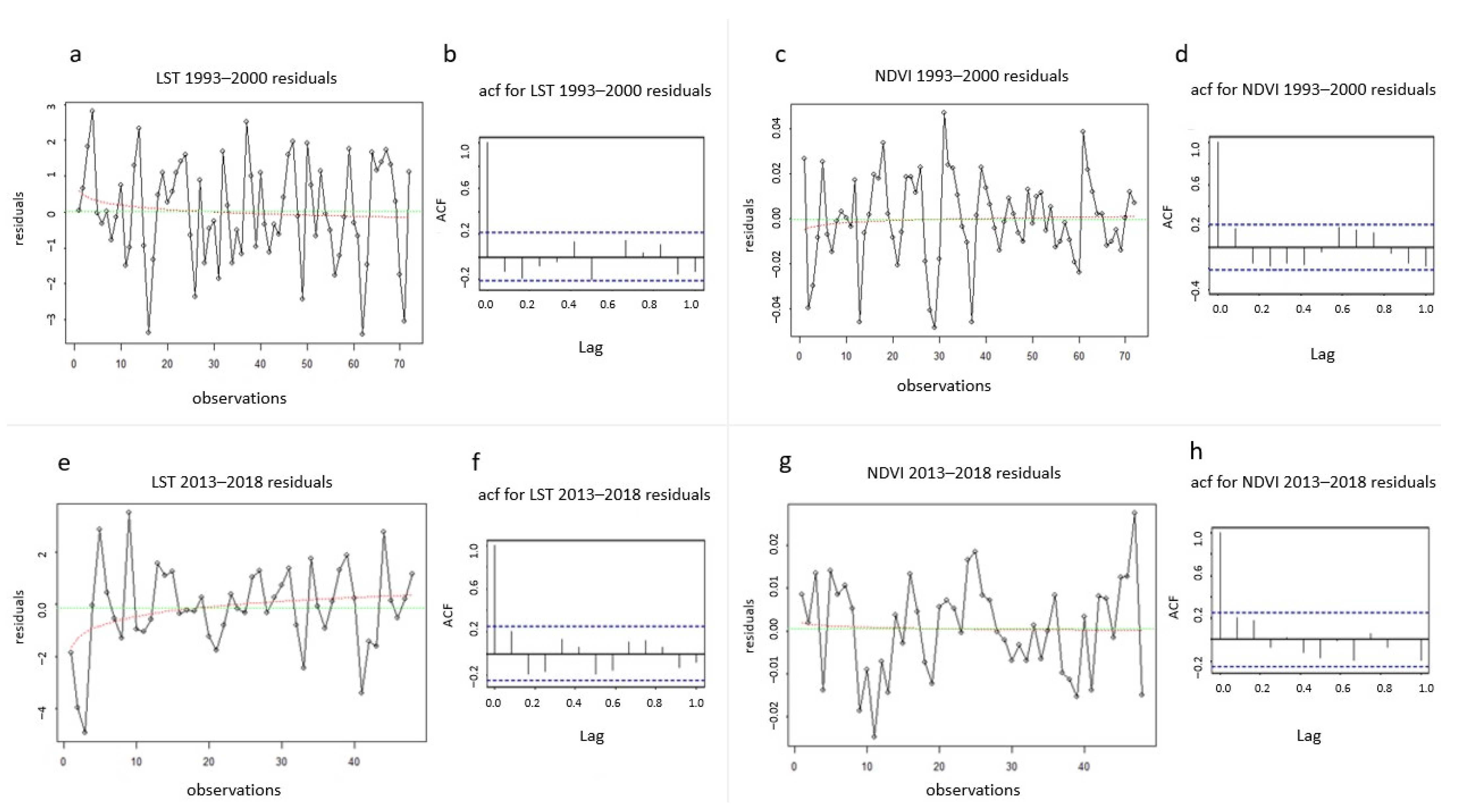
The residuals of the time series that were examined within this study behaved normally as shown by the plots (Figure 15) that highlighted the residuals were randomly distributed around the value 0 confirmed the correctness of the choice of the additive decomposition model.
The residuals for the LST (Figure 15a,b,e,f) and NDVI (Figure 15c,d,g,h) time series did not present autocorrelation, therefore, the estimated quantities, such as the variations of the model coefficients but also the hypothesis tests were unbiased.
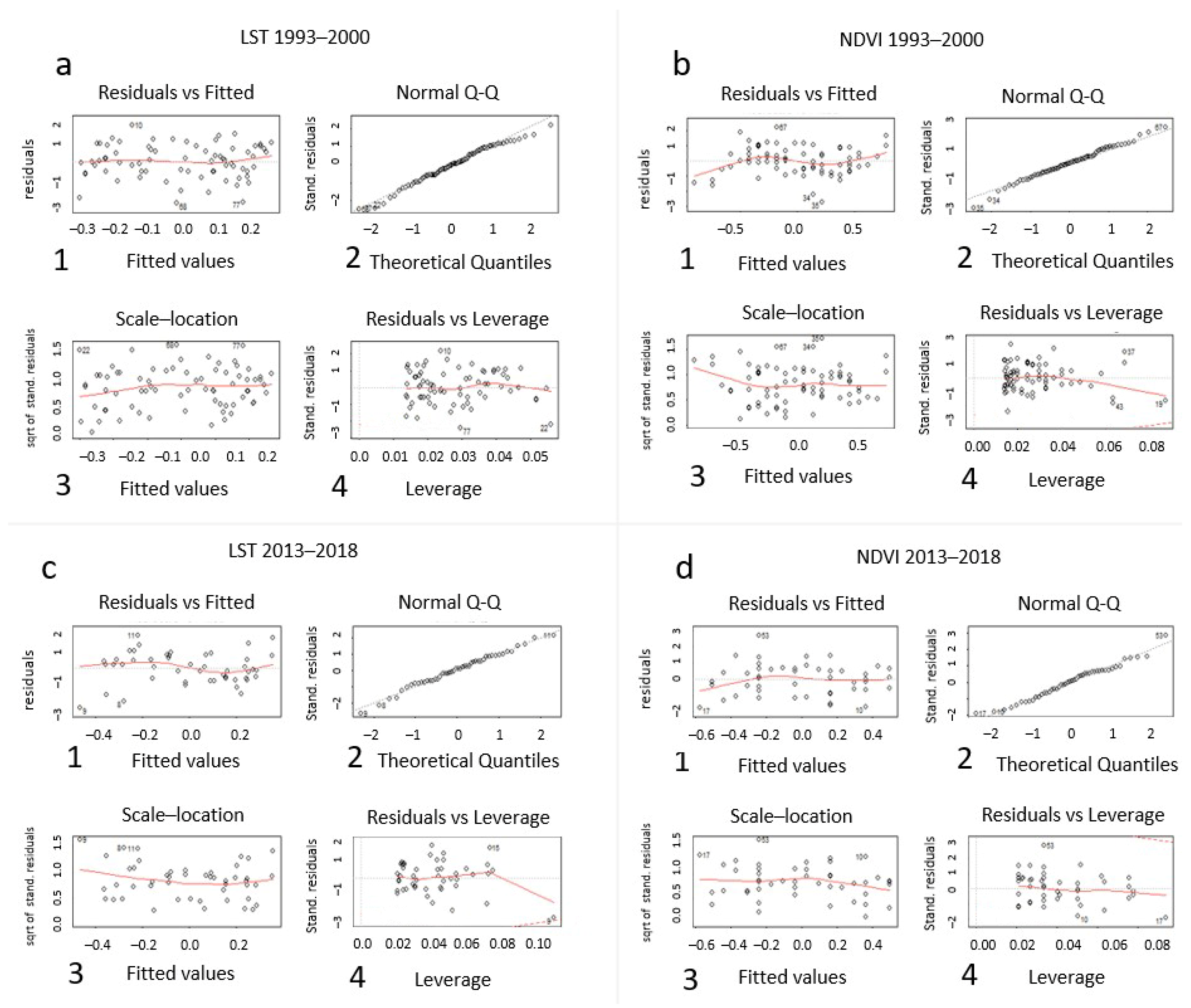
Additional controls on the residuals, by creating the residuals versus fits scatter plot, (Figure 16(a1,b1,c1,d1)), with residuals on the y-axis and fitted values on the x-axis, showed a linearity and equal error variances. This result is clearly indicated by the scale—location plots, (Figure 16(a3,b3,c3,d3)), which show that residuals are spread equally along the ranges of LST and NDVI values. Consequently, the assumption of homoscedasticity is valid in the decomposition models that were used within this study. The residuals—leverage plots, (Figure 16(a4,b4,c4,d4)), show how the spread of standardized residuals changes as the leverage increases, so we can observe that the model has not heteroscedasticity and very few important points with high leverage exist. These points are mainly leverage (i.e., have values of x that are far away from the mean of x) and influential observations that changes the slope of the fitted line.
Τhe cross-correlation coefficient for the 1993–2000 and 2013–2018 time series between the LST and NDVI residuals for each month was calculated. Nevertheless, the 1993–2000 time series started in March 1993 and ended in February 2000, while the 2013–2018 time series started in April 2013 and ended in March 2018 and this maybe that affect the results of the residuals analysis. For that reason, to obtain reliable results and a complete seasonal number of observations of the residual analysis, the time series 1994–1999 and 2014–2017 were used, so that they started in January and ended in December. The level of zero correlation is shown in the graph with the red horizontal line (Figure 17a,b). For both periods, during February and August, the values of the residuals were positively correlated (red circle), while for all the other months the residuals were negative. An exception was the correlation for April (red arrow), where the positive value 0.36 in the time series 1994–1999 switched to a negative value (−0.66) in the time series 2014–2017 (Figure 17b). Indeed, a thorough observation of the LST (Figure 17c,e) and NDVI (Figure 17d,f) seasonal graphs revealed that April presented a mean NDVI value of about 0.46 with a mean LST value 26 °C for the 1994–1999 time series, while it presented a mean NDVI value of about 0.56 with a mean LST value 24.5 °C for the 2014–2017 time series. The study of the residuals highlighted this change which could not be easily observed in the seasonal graphs. It is interesting that residual analysis can potentially reveal some changes that are not apparent in the seasonal graphs.

4.6. Computational Requirements and Limitations

Free platform-independent and open-source software has been used throughout this work. The Landsat images were downloaded using the bulk download tool of USGS. The pre-processing and processing of the images (i.e., cloud masking, NDVI and temperature calculations, mean value and standard deviation calculations, and statistical data storage) were carried out automatically using a combination of python and GDAL programs and appropriate batch scripts. The time series analysis was carried out using the R programming language.
A basic computing setup of a desktop computer was used to perform the processing and the analysis. There are no limitations for extending the analysis to larger areas or to a longer period, other than the image download time, the temporary storage space that is required for the downloaded images, and the pre-processing and processing time. One limitation that cannot be overcome of course is the satellite data availability. If this work was to be extended to very large areas, parallel processing would have to be used to timely retrieve the statistical data and be able to carry out the time series analysis. Setting up the pre-processing and processing steps on a cloud service that has all the relevant satellite data available online, would vastly increase the processing speed and would be highly recommended for large scale processing. The time series decomposition can also be an automated process in R or python, but the results have to be carefully examined and evaluated. Once new data become available, the time series analysis can be populated by automatic downloading and processing of the new data (with crontab jobs and appropriate python scripts) and rerunning the analysis on top of the previous results.

5. Conclusions

The supply of forest ecosystems for a country is large and multifaceted. Climate change is related to degradation of natural ecosystems, while forests do not only provide environmental benefits but also economic and social, justifying the need for maintaining healthy forests. The composition of forests is changing, so it is important to monitor trends and understand how our forests will be affected in the future by the increase or decrease of the land surface temperature. This is important for advocacy and policy-making, forest preservation, and management (e.g., establishment of protected zones).
In this study it was shown that Big Earth Observation Data, specifically Landsat imagery data, can be used to efficiently monitor the land surface temperature (LST) changes and how these changes affect the coniferous Paphos forest, Cyprus. The normalized difference vegetation index (NDVI) was selected as an indicator for defining the vegetation condition. As Landsat data were acquired from different satellite missions, the entire period of investigation was divided into two district time periods, 1993–2000 and 2013–2018. The two time series containing the monthly mean values of LST and NDVI, respectively, were calculated during each of these time periods for the study area. The missing values of the time series were completed with the use of the Kalman filter, which satisfactorily normalizes the overall impact that is created by high-leverage observations. This study found only two points that were much higher than the upper limit of the confidence level using Cook’s distance.
In this work, the Cook’s distance was used to detect the influential points in the time series and their effect in the decomposition of the time series was studied. The results that were generated by the decomposition model and the BFAST algorithm, were compared to produce reliable conclusions that were related to abrupt changes in LST and NDVI time series. The results that were produced by cross-correlation functions and cross-variograms of LST and NDVI were also compared to examine the relationships of NDVI time-series to past lags of LST time-series. Satellite, meteorological, and environmental data were combined to interpret changes in Paphos forest, Cyprus.
The research yields interesting results about the study area. Statistical analysis of the air temperature data showed an almost constant mean negative deviation of about 6.50 degrees from the respective LST mean during the period 1993–2018. A slight upward trend was identified in the air temperature data. The decomposition analysis showed a slight increase of 0.3% in the aerial temperature time series for the period 1992–2016, a decrease of 2.7% in the LST for the period 1993–2000, and an increase of 4.6% in the LST in the period 2013–2018. Trends in the LST time series were interpreted by changes in the precipitation and aerial temperature. Decomposition analysis on the NDVI time series showed that the NDVI trend was negatively correlated to the LST trend for both periods; implying that even a slight increase in LST over the years causes a decrease in the NDVI values and vice versa.
The BFAST algorithm successfully detected the break points in the trend line. A significant increase in the LST trend line was identified in November 1998, which was interpreted by changes in the LST and the aerial temperature. In the NDVI time series, abrupt increases were observed in October 1994 and May 2014, caused by increased rainfall and favorable for the vegetation air and land surface temperatures. Furthermore, the increase in May 2014 that lasted until December 2015, may be linked to reduced acts of Thaumatopea pityocampa due to low temperatures in the earlier autumn months. An abrupt decrease was detected in December 2015 that was probably caused by the locust invasion that occurred in the island earlier that year.
There were two influential points that were detected in the LST 1993–2000 time series using the Cook’s distance. New values for these points were estimated using the Kalman filter. The additive decomposition model and the BFAST algorithm were then applied on the updated time series. The study indicated that the influential points affect locally and slightly the trend component of the decomposition model, while the break points remained the same.
Auto correlation functions indicated a similar pattern for the LST and NDVI time series in the forest of Paphos. Strong negative correlations on the sixth month were observed for both periods. The analysis of the cross-correlation of the LST and NDVI parameters showed a strong negative correlation up to the first two lags. This correlation became positive after the next two lags. A positive correlation appeared for month lags 4, 5, 6, 7, and 8. The result was observed in both time series, 1993–2000 and 2013–2018, respectively, and confirmed by cross-variograms.
The residual analysis within this study indicated the suitability of the models. Τhe cross-correlation coefficient for the 1993–2000 and 2013–2018 time series between the LST and NDVI residuals for each month identified cross-correlations that were not similar for the two time periods for the month of April. This may also be linked to a reduced act of Thaumatopea pityocampa in the years 2014 and 2015.
In future work we would like to experiment with other gap-filling methods, build prediction models, embed more data, and compare results with data from other study areas.

Author Contributions

Conceptualization all authors; methodology, V.A. and V.K.; software, V.A. and P.K.; validation, V.A.; formal analysis, V.A. and V.K.; investigation, V.A. and V.T.; data curation, P.K., V.T. and V.A.; writing—original draft preparation, V.A.; writing—review and editing, all authors; visualization, V.A. and V.K.; supervision, V.K.; funding acquisition, V.K. All authors have read and agreed to the published version of the manuscript.

Funding

This study was funded by the “ASTARTE” (EXCELLENCE/0918/0341) research, which is co-financed by the European Regional Development Fund and the Republic of Cyprus through the Research Innovation Foundation.

Data Availability Statement

All the source satellite data are publicly available online through the USGS portal (https://earthexplorer.usgs.gov, accessed on 31 January 2022). The meteorological data have been provided by the Department of Meteorology of Nicosia, Cyprus. The data generated in this study as well as the developed software are available upon request.

Acknowledgments

The authors would like to thank the Department of Meteorology of Nicosia, Cyprus, for the provision of the meteorological data. We also like to thank the United States Geological Survey (USGS) for supplying the Landsat images and the anonymous reviewers for their contribution to the improvement of the overall quality of the manuscript.

Conflicts of Interest

The authors declare no conflict of interest.

References

  1. Solanky, V.; Singh, S.; Katiyar, S.K. Land Surface Temperature Estimation Using Remote Sensing Data. In Hydrologic Modeling; Springer: Singapore, 2018. [Google Scholar]
  2. Dash, P. Land Surface Temperature and Emissivity Retrieval from Satellite Measurements; Forschungszentrum Karlsruhe: Karlsruhe, Germany, 2005; pp. 1–99. [Google Scholar]
  3. Yang, J.; Ren, J.; Sun, D.; Xiao, X.; Xia, J.; Jin, C.; Li, X. Understanding land surface temperature impact factors based on local climate zones. Sustain. Cities Soc. 2021, 69, 102818. [Google Scholar] [CrossRef]
  4. Ali, S.B.; Patnaik, S.; Madguni, O. Microclimate land surface temperatures across urban land use/ land cover forms. Glob. J. Environ. Sci. Manag. 2017, 3, 231–242. [Google Scholar] [CrossRef]
  5. Rajendran, P.; Mani, D.K. Estimation of Spatial Variability of Land Surface Temperature using Landsat 8 Imagery. Int. J. Eng. Sci. 2015, 4, 19–23. [Google Scholar]
  6. Han, H.; Bai, J.; Ma, G.; Yan, J. Vegetation phenological changes in multiple landforms and responses to climate change. ISPRS Int. J. Geo-Inf. 2020, 9, 111. [Google Scholar] [CrossRef] [Green Version]
  7. Yan, Y.; Mao, K.; Shi, J.; Piao, S.; Shen, X.; Dozier, J.; Liu, Y.; Ren, H.L.; Bao, Q. Driving forces of land surface temperature anomalous changes in North America in 2002–2018. Sci. Rep. 2020, 10, 6931. [Google Scholar] [CrossRef]
  8. Akinyemi, F.O.; Ikanyeng, M.; Muro, J. Land cover change effects on land surface temperature trends in an African urbanizing dryland region. City Environ. Interact. 2019, 4, 100029. [Google Scholar] [CrossRef]
  9. Dang, T.; Yue, P.; Bachofer, F.; Wang, M.; Zhang, M. Monitoring land surface temperature change with landsat images during dry seasons in Bac Binh, Vietnam. Remote Sens. 2020, 12, 4067. [Google Scholar] [CrossRef]
  10. Heinemann, S.; Siegmann, B.; Thonfeld, F.; Muro, J.; Jedmowski, C.; Kemna, A.; Kraska, T.; Muller, O.; Schultz, J.; Udelhoven, T.; et al. Land surface temperature retrieval for agricultural areas using a novel UAV platform equipped with a thermal infrared and multispectral sensor. Remote Sens. 2020, 12, 1075. [Google Scholar] [CrossRef] [Green Version]
  11. How, D.; Aik, J.; Ismail, M.H.; Muharam, F.M. Land Use/Land Cover Changes and the Relationship. Land 2020, 9, 372. [Google Scholar]
  12. Lambin, E.F.; Ehrlich, D. The surface temperature-vegetation index space for land cover and land-cover change analysis. Int. J. Remote Sens. 1996, 17, 463–487. [Google Scholar] [CrossRef]
  13. Mohd Jaafar, W.S.W.; Maulud, K.N.A.; Muhmad Kamarulzaman, A.M.; Raihan, A.; Sah, S.M.; Ahmad, A.; Maizah Saad, S.N.; Mohd Azmi, A.T.; Syukri, N.K.A.J.; Khan, W.R. The influence of deforestation on land surface temperature-A case study of Perak and Kedah, Malaysia. Forests 2020, 11, 670. [Google Scholar] [CrossRef]
  14. Rodrigues, C.; Teodoro, A.C.M. Relationship between the land surface temperature and the vegetation proportion to identify Heat Islands. Case study of Brasília (Brazil). In Proceedings of the Earth Resources and Environmental Remote Sensing/GIS Applications XI, Online, 21–25 September 2020; Schulz, K., Nikolakopoulos, K.G., Michel, U., Eds.; SPIE: Bellingham, WA, USA, 2020; p. 34. Available online: https://www.spiedigitallibrary.org/conference-proceedings-of-spie/11534/1153411/Relationship-between-the-land-surface-temperature-and-the-vegetation-proportion/10.1117/12.2572802.short?SSO=1 (accessed on 31 January 2022). [CrossRef]
  15. Guha, S.; Govil, H. An assessment on the relationship between land surface temperature and normalized difference vegetation index. Environ. Dev. Sustain. 2021, 23, 1944–1963. [Google Scholar] [CrossRef]
  16. Tang, B.; Zhao, X.; Zhao, W. Local effects of forests on temperatures across Europe. Remote Sens. 2018, 10, 529. [Google Scholar] [CrossRef] [Green Version]
  17. Macarof, P.; Groza, S.; Statescu, F. Investiganting Correlation LST and Vegetation Indices Using Landsat Images for the Warmest Month: A Case Study of Iasi County. Ann. Valahia Univ. Targoviste, Geogr. Ser. 2018, 18, 33–40. [Google Scholar] [CrossRef] [Green Version]
  18. Liu, Y.; Yamaguchi, Y.; Ke, C. Reducing the discrepancy between ASTER and MODIS land surface temperature products. Sensors 2007, 7, 3043–3057. [Google Scholar] [CrossRef] [PubMed] [Green Version]
  19. Meng, X.; Cheng, J.; Zhao, S.; Liu, S.; Yao, Y. Estimating land surface temperature from Landsat-8 data using the NOAA JPSS enterprise algorithm. Remote Sens. 2019, 11, 155. [Google Scholar] [CrossRef] [Green Version]
  20. Abdul Athick, A.S.M.; Shankar, K.; Naqvi, H.R. Data on time series analysis of land surface temperature variation in response to vegetation indices in twelve Wereda of Ethiopia using mono window, split window algorithm and spectral radiance model. Data Br. 2019, 27, 104773. [Google Scholar] [CrossRef] [PubMed]
  21. Quan, J.; Zhan, W.; Chen, Y.; Wang, M.; Wang, J. Time series decomposition of remotely sensed land surface temperature and investigation of trens and seasonal variations in surface urban heat islands. Nature 1955, 175, 238. [Google Scholar] [CrossRef]
  22. Qiu, S.; Zhu, Z.; He, B. Fmask 4.0: Improved cloud and cloud shadow detection in Landsats 4–8 and Sentinel-2 imagery. Remote Sens. Environ. 2019, 231, 111205. [Google Scholar] [CrossRef]
  23. Saputra, M.D.; Hadi, A.F.; Riski, A.; Anggraeni, D. Handling Missing Values and Unusual Observations in Statistical Downscaling Using Kalman Filter. J. Phys. Conf. Ser. 2021, 1863, 012035. [Google Scholar] [CrossRef]
  24. Muflihah Rizky Yudha Pahlawan Perbandingan Teknik Interpolasi Berbasis R Dalam Estimasi Data Curah Hujan Bulanan Yang Hilang Di Sulawesi Comparison of R-Based Interpolation Techniques To Estimate. 2017, pp. 107–111. Available online: http://puslitbang.bmkg.go.id/jmg/index.php/jmg/article/download/343/pdf (accessed on 17 February 2022).
  25. Welch, G.; Bishop, G. An Introduction to the Kalman Filter; ACM, Inc.: Tipp City, OH, USA, 2001. [Google Scholar]
  26. Kumar, D.; Shekhar, S. Statistical analysis of land surface temperature-vegetation indexes relationship through thermal remote sensing. Ecotoxicol. Environ. Saf. 2015, 121, 39–44. [Google Scholar] [CrossRef] [PubMed]
  27. Potter, C.; Coppernoll-Houston, D. Controls on land surface temperature in deserts of southern california derived from MODIS satellite time series analysis, 2000 to 2018. Climate 2019, 7, 32. [Google Scholar] [CrossRef] [Green Version]
  28. Lambert, J.; Drenou, C.; Denux, J.P.; Balent, G.; Cheret, V. Monitoring forest decline through remote sensing time series analysis. GIScience Remote Sens. 2013, 50, 437–457. [Google Scholar] [CrossRef]
  29. Ben Abbes, A.; Bounouh, O.; Farah, I.R.; de Jong, R.; Martínez, B. Comparative study of three satellite image time-series decomposition methods for vegetation change detection. Eur. J. Remote Sens. 2018, 51, 607–615. [Google Scholar] [CrossRef] [Green Version]
  30. Schelter, B.; Winterhalder, M. Handbook of Time Series Analysis; Wiley-VCH: Berlin, Germany, 2006; ISBN 9780471363552. [Google Scholar]
  31. Dagum, E.B. Time Series Modeling and Decomposition. Statistica 2010, 70, 433–457. [Google Scholar] [CrossRef]
  32. Sutcliffe, A. X11 Time Series Decomposition and Sampling Errors; Australian Bureau of Statistics: Melbourne, Australia, 1993.
  33. Cleveland, W.R.; Cleveland, J.; McRae, I.T. Statistics Sweden. J. Off. Stat. 1990, 6, 3–73. [Google Scholar]
  34. Verbesselt, J.; Hyndman, R.; Zeileis, A.; Culvenor, D. Phenological Change Detection While Accounting for Abrupt and Gradual Trends in Satellite Image Time Series. Remote Sens. Environ. 2010, 114, 2970–2980. [Google Scholar] [CrossRef] [Green Version]
  35. Rhif, M.; Ben Abbes, A.; Martinez, B.; Farah, I.R. An improved trend vegetation analysis for non-stationary NDVI time series based on wavelet transform. Environ. Sci. Pollut. Res. 2020, 28, 46603–46613. [Google Scholar] [CrossRef]
  36. Zachariadis, T. Climate Change in Cyprus: Impacts and Adaptation Policies. Cyprus Econ. Policy Rev. 2012, 16, 21–37. [Google Scholar]
  37. Miltiadou, M.; Antoniou, E.; Theocharidis, C.; Danezis, C. Do people understand and observe the effects of climate crisis on forests? The case study of cyprus. Forests 2021, 12, 1152. [Google Scholar] [CrossRef]
  38. Republic of Cyprus, Ministry of Agriculture; N.R. and E. Paphos Forest Management Plan: Nicosia, Cyprus, 2011.
  39. Hansen, M.C.; Potapov, P.V.; Moore, R.; Hancher, M.; Turubanova, S.A.; Tyukavina, A.; Thau, D.; Stehman, S.V.; Goetz, S.J.; Loveland, T.R.; et al. University of M. High-Resolution Global Maps of 21st-Century Forest Cover Change. Science 2013, 342, 850–853. [Google Scholar] [CrossRef] [PubMed] [Green Version]
  40. Jennings, R.C. The locust problem in cyprus. Bull. Sch. Orient. African Stud. 1988, 51, 279–313. [Google Scholar] [CrossRef]
  41. Hódar, J.A.; Castro, J.; Zamora, R. Pine processionary caterpillar Thaumetopoea pityocampa as a new threat for relict Mediterranean Scots pine forests under climatic warming. Biol. Conserv. 2003, 110, 123–129. [Google Scholar] [CrossRef]
  42. Invasive Species Compendium Thaumetopoea Pityocampa (Pine Processionary). Available online: https://www.cabi.org/isc/datasheet/53501#toenvironments (accessed on 2 February 2022).
  43. SOER Country Profile—Distinguishing Factors (Cyprus). Available online: https://www.eea.europa.eu/soer/2010/countries/cy/country-introduction-cyprus (accessed on 31 January 2022).
  44. Moritz, S.; Bartz-Beielstein, T. ImputeTS: Time series missing value imputation in R. R J. 2017, 9, 207–218. [Google Scholar] [CrossRef] [Green Version]
  45. Dennis Cook, S.W. Residuals and Influence in Regression; Chapman and Hall: New York, NY, USA, 1982. [Google Scholar]
  46. Hilas, C.S.; Goudos, S.K.; Sahalos, J.N. Seasonal decomposition and forecasting of telecommunication data: A comparative case study. Technol. Forecast. Soc. Change 2006, 73, 495–509. [Google Scholar] [CrossRef]
  47. Mutiibwa, D.; Strachan, S.; Albright, T. Land Surface Temperature and Surface Air Temperature in Complex Terrain. IEEE J. Sel. Top. Appl. Earth Obs. Remote Sens. 2015, 8, 4762–4774. [Google Scholar] [CrossRef]
  48. Xu, D. Compare NDVI Extracted from Landsat 8 Imagery with that from Landsat 7 Imagery. Am. J. Remote Sens. 2014, 2, 10. [Google Scholar] [CrossRef] [Green Version]
  49. Vogelmann, J.E.; Helder, D.; Morfitt, R.; Choate, M.J.; Merchant, J.W.; Bulley, H. Effects of Landsat 5 Thematic Mapper and Landsat 7 Enhanced Thematic Mapper plus radiometric and geometric calibrations and corrections on landscape characterization. Remote Sens. Environ. 2001, 78, 55–70. [Google Scholar] [CrossRef] [Green Version]
  50. Schachat, S.R.; Labandeira, C.C.; Maccracken, S.A. The importance of sampling standardization for comparisons of insect herbivory in deep time: A case study from the late palaeozoic. R. Soc. Open Sci. 2018, 5, 171991. [Google Scholar] [CrossRef] [Green Version]
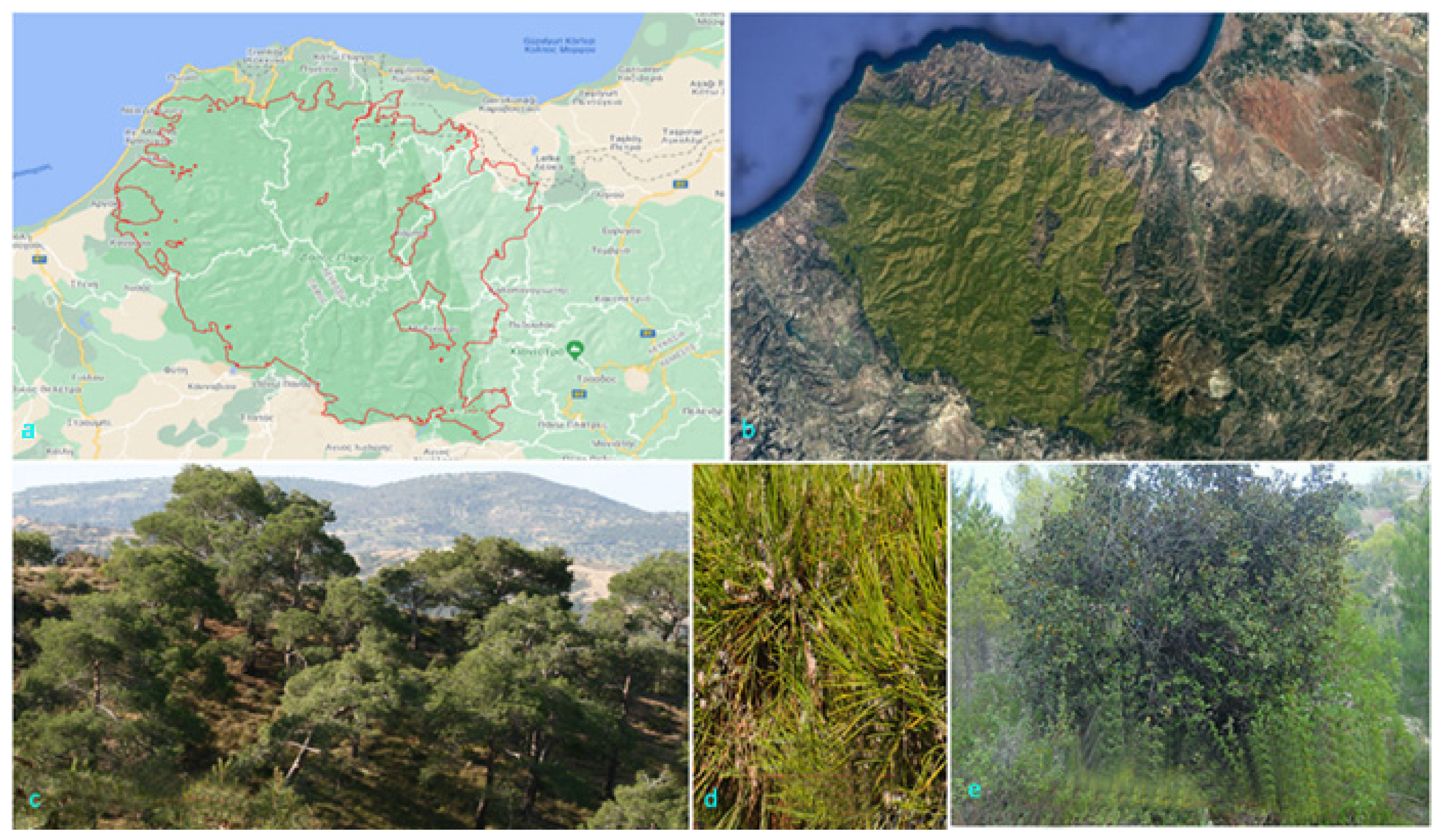
Figure 1. The study area with: (a) Paphos forest boundaries; (b) Paphos forest in RGB with natural colors from Google Earth imagery; (c) Pinus brutia; (d) Pinus brutia foliage; (e) Quercus alnifolia the main substrate in Pathos forest.
Remotesensing 14 01010 g001
Figure 2. Flow chart of the methodology.
Remotesensing 14 01010 g002
Figure 3. Diagrams for the LST 1993–2000 time series: (a) Cook’s distance with MA interpolated values; (b) Cook’s distance with the Kalman filter interpolated values; (c) comparative graph where the blue color are the values after MA and where the red color are those after the Kalman filter interpolation. The points that are shown by arrows are the ones with large influence as it was indicated by the Cook’s distance.
Remotesensing 14 01010 g003
Figure 4. The Cook’s distance for the updated LST 1993–2000 time series.
Remotesensing 14 01010 g004
Figure 5. Density annual plots for: (a) LST time series 2014–2017; (b) aerial temperature time series 2014–2015; (c) NDVI time series 2014–2017; (d) LST time series 1994–1999, (e) aerial temperature time series 1994–1999, and (f) NDVI time series 1994–1999.
Remotesensing 14 01010 g005
Figure 6. Diagrams about the aerial temperature 1992–2016 time series: (a) ergodic mean monthly values; (b) boxplot graph showing the mean (red dot) and median (black dash) values volatility, and (c) the monthly values.
Remotesensing 14 01010 g006
Figure 7. The LST trend component after decomposition: (a) Trendline (blue line) for the 1993–2000 time series with equation y = 24.818 − 0.0026929x. The arrows point to the areas of trend breakpoints; (b) Trendline (blue line) for the 2013–2018 time series with equation y = 23.17 + 0.046534x.
Remotesensing 14 01010 g007
Figure 8. The BFAST algorithm application for the 1993–2000 time series: (a) decomposition with BFAST, one trend breakpoint showed in the blue circle over the trendline (red line); (b) classical decomposition; (c) trend component (black line) with its trendline (red line) and an arrow showing the break; and (d) the trend component (black line) overlying the trendline from the BFAST algorithm (red line) with the blue circle indicating the break.
Remotesensing 14 01010 g008
Figure 9. The trend of the updated time series (black) and the trend of the time series with the influential observations (red).
Remotesensing 14 01010 g009
Figure 10. The NDVI trend component after decomposition: (a) The trendline (blue line) for the 1993–2000 time series with equation y = 0.44164 + 0.00026747x; (b) The trendline (blue line) for the 2013–2018 time series with equation y = 0.56516 − 0.00033242x. The arrows point to the areas of interesting trend breakpoints.
Remotesensing 14 01010 g010
Figure 11. (a) The trend breakpoint for NDVI 1993–2000 time series is shown in the blue circle over the trendline, (b) decomposition of the NDVI 1993–2000 time series. The blue arrow points to the area of the breakpoint, (c) the NDVI 1993–2000 trend component (black line) overlaid over the trendline that was derived from the BFAST algorithm (red line). The blue circle indicates the break, (d) the two trend breakpoints for the NDVI 2013–2018 time series are shown in blue circles, (e) the decomposition of the NDVI 2013–2018 time series. The blue arrows point to the breakpoints, (f) the NDVI 2013–2018 trend component (red line) overlaid over the trendline that was derived from the BFAST algorithm (black line). The blue circle indicates the breaks.
Remotesensing 14 01010 g011
Figure 12. (a) Autocorrelation graph for the LST time series 1993–2000; (b) autocorrelation graph for the NDVI time series 1993–2000; (c) autocorrelation graph for the LST time series 2013–2018; (d) autocorrelation graph for the NDVI time series 2013–2018; (e) lag plots (for lag = 1 until lag = 15) for the LST time series 1993–2000 and (f) lag plots for the NDVI time series 1993–2000.
Remotesensing 14 01010 g012
Figure 13. (a) Cross-correlation graph for the LST 1993–2000 and the NDVI 1993–2000; (b) cross-correlation graph for the LST 2013–2018 and the NDVI 2013–2018; (c) a grid of scatterplots of the LST versus the NDVI 1993–2000 time series.
Remotesensing 14 01010 g013
Figure 14. Cross-variogram for (a) the LST and the NDVI 1993–2000 time series; (b) the LST and the NDVI 2013–2018 time series.
Remotesensing 14 01010 g014
Figure 15. (a) The LST 1993–2000 residuals plot with the mean value (green line) and ergodic mean (red line); (b) autocorrelation plot for the LST 1993–2000 residuals; (c) The NDVI 1993–2000 residuals plot with the mean value (green line) and ergodic mean (red line); (d) autocorrelation plot for the NDVI 1993–2000 residuals; (e) LST 2013–2018 residuals plot with the mean value (green line) and ergodic mean (red line); (f) autocorrelation plot for the LST 2013–2018 residuals; (g) The NDVI 2013–2018 residuals plot with the mean value (green line) and ergodic mean (red line); (h) autocorrelation plot for the NDVI 2013–2018 residuals.
Remotesensing 14 01010 g015
Figure 16. The time series for: (a) LST 1993–2000; (b) NDVI 1993–2000; (c) LST 2013–2018; (d) NDVI 2013–2018. For each time series plots include: (1) a residuals vs. fitted plot; (2) a normal Q-Q plot; (3) a scale-location plot, and (4) a residuals vs. leverage plot.
Remotesensing 14 01010 g016
Figure 17. Cross-correlation coefficients plots between the LST and the NDVI residuals per month: (a) in the 1994–1999 time series; (b) in the 2014–2017 time series. Seasonal plots: (c) for the LST 1994–1999; (d) for the NDVI 1994–1999; (e) for the LST 2014–2017; and (f) for the NDVI 2014–2017. In (cf) diagrams, there is a black dashed line indicating the month of April, which showed a peculiar behavior in the correlation. In these diagrams, the numbers 1,2,3,4,5,6 indicate the years 1994, 1995, 1996, 1997, 1998, 1999, for the 1994–1999 time series and the years 2014, 2015, 2016, 2017, for the 2014–2017 time series.
Remotesensing 14 01010 g017
Table 1. Basic statistics for the LST, NDVI, and aerial temperature time series.
Time SeriesMin.1st QuantileMedianMean3rd QuantileMax.Stdev
LST 1993–20008.4018.3825.5024.8932.2536.807.722
NDVI 1993–20000.340.410.450.450.490.550.049
aerial 1993–20005.7010.5718.2018.4425.5031.707.755
LST 2013–20189.5017.3225.8525.0132.7338.608.892
NDVI 2013–20180.470.520.560.560.590.630.044
aerial 2013–20167.3013.1019.0519.0024.4330.107.108
Publisher’s Note: MDPI stays neutral with regard to jurisdictional claims in published maps and institutional affiliations.